Chapter 2: Structure of Atom
Late one night in his Copenhagen study in 1913, a young Danish physicist named Niels Bohr was staring at a set of numbers that made no sense. Hydrogen gas, when heated inside a glass tube, did not glow with a smooth rainbow of colour. Instead it threw out light at only a few sharp, fixed wavelengths — a red line, a blue-green line, a violet line — always the same, never anything in between. Why would an atom be so fussy about which colours it emitted?
The puzzle went deeper. According to the physics of the day, an electron circling the nucleus should spiral inward and crash into it within a hundred-millionth of a second, and the atom should collapse. Yet atoms plainly did not collapse. The chair Bohr sat on, the paper he wrote on, his own hands — all were made of atoms that had survived for billions of years.
Bohr made a daring guess. What if the electron was allowed to travel only in certain fixed orbits, each with a definite energy, and light was released only when it jumped from one to another? Suddenly the sharp lines of hydrogen fell into place, matching a formula spectroscopists had found years earlier but could not explain. A guess about invisible electrons had predicted the visible colours of glowing gas — and the modern picture of the atom had begun.
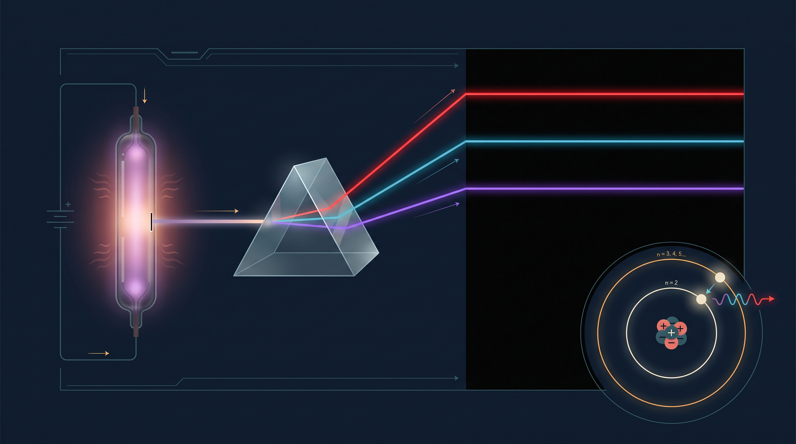
Fig. 2.0 – The hydrogen line spectrum and Bohr’s atomic model.
By the end of this chapter you will be able to reason your way to the answers to all of these questions.
2.1 Discovery of Sub-atomic Particles
For a long time, scientists pictured the atom exactly as its name suggested — the smallest, uncuttable, indivisible piece of matter. The word atom itself comes from a Greek root meaning “uncut-able.” Yet by the end of the nineteenth century, a series of experiments showed something remarkable: the atom is not the final unit of matter at all. It is built out of even smaller particles that carry electric charge. These smaller particles are called sub-atomic particles, and the three most important are the electron, the proton, and the neutron.
Most of the early clues came from experiments on passing electricity through gases. Before we follow those experiments, one simple rule about electric charge must be kept firmly in mind, because it explains almost everything that follows: like charges repel each other, and unlike charges attract each other. Two negative charges push apart; a positive and a negative charge pull together.
2.1.1 Discovery of Electron
The trail began with electricity and matter behaving in surprising ways together. In 1830, Michael Faraday showed that when electricity is passed through a solution of an electrolyte (a substance that conducts electricity in solution), chemical reactions take place at the electrodes, and matter is set free or deposited there. This hinted that electricity itself might be made of particles — that it has a “particulate” nature — rather than being a smooth, continuous fluid.
To probe this further, scientists in the mid-1850s, led again by Faraday, began studying electrical discharge through partially evacuated glass tubes. These are called cathode ray discharge tubes. A cathode ray tube is a sealed glass tube containing two thin metal plates called electrodes. The set-up is drawn in Fig. 2.1.
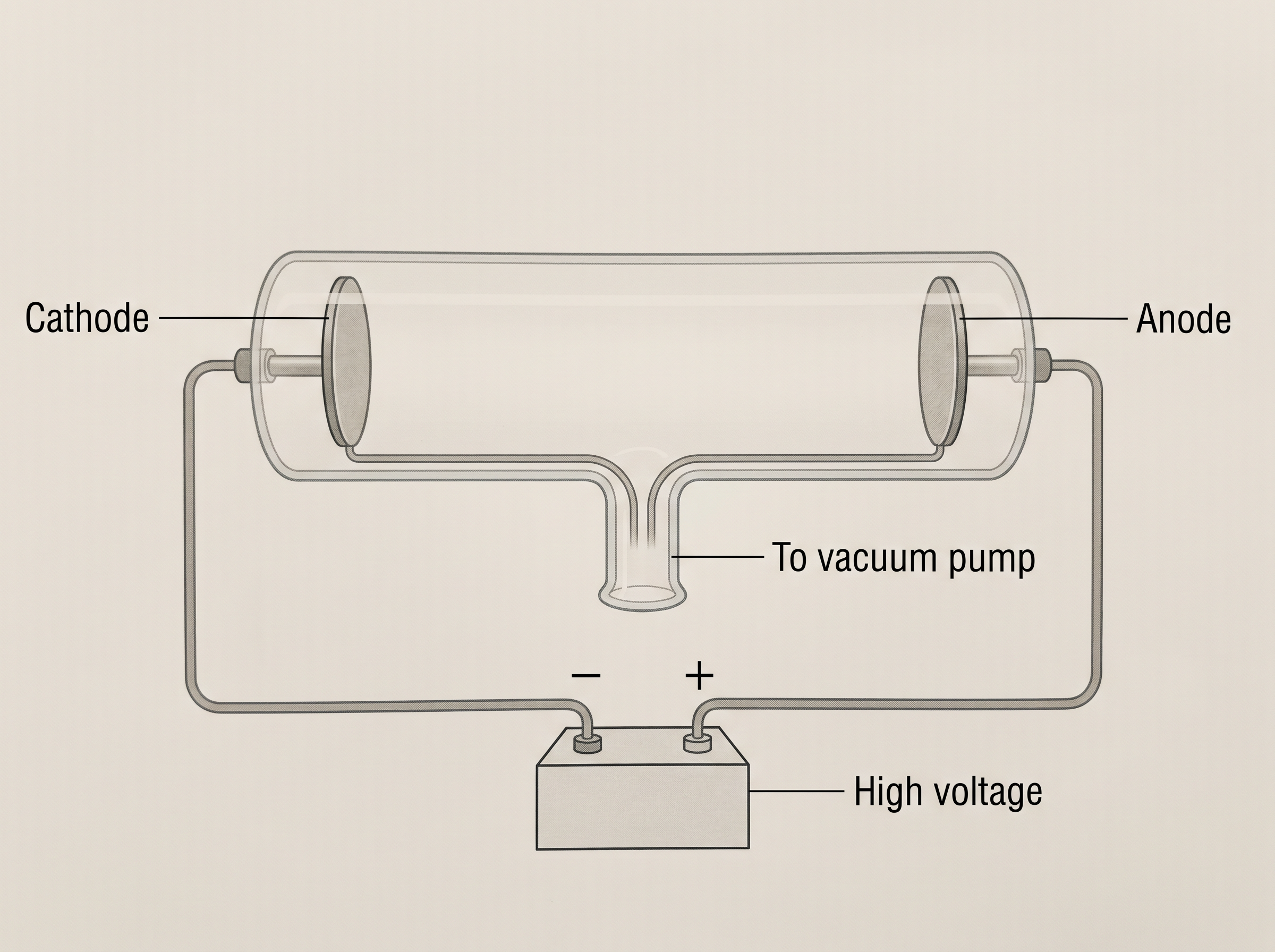
Fig. 2.1(a) – Cathode ray discharge tube.
The discharge could be seen only under two special conditions together: very low gas pressure inside the tube, and a very high voltage across the electrodes. The pressure of the gas could be adjusted by pumping air out of the tube.
When a high enough voltage is applied, current begins to flow. It flows as a stream of particles that travel through the tube from the negative electrode, the cathode, to the positive electrode, the anode. These streams were named cathode rays or cathode ray particles.
To confirm the direction of this flow, a hole was made in the anode and the glass behind it was coated with a phosphorescent material, zinc sulphide. When the rays passed through the hole in the anode and struck this coating, they produced a bright glowing spot, as shown in Fig. 2.2(b). This proved the rays kept moving in a straight line past the anode.
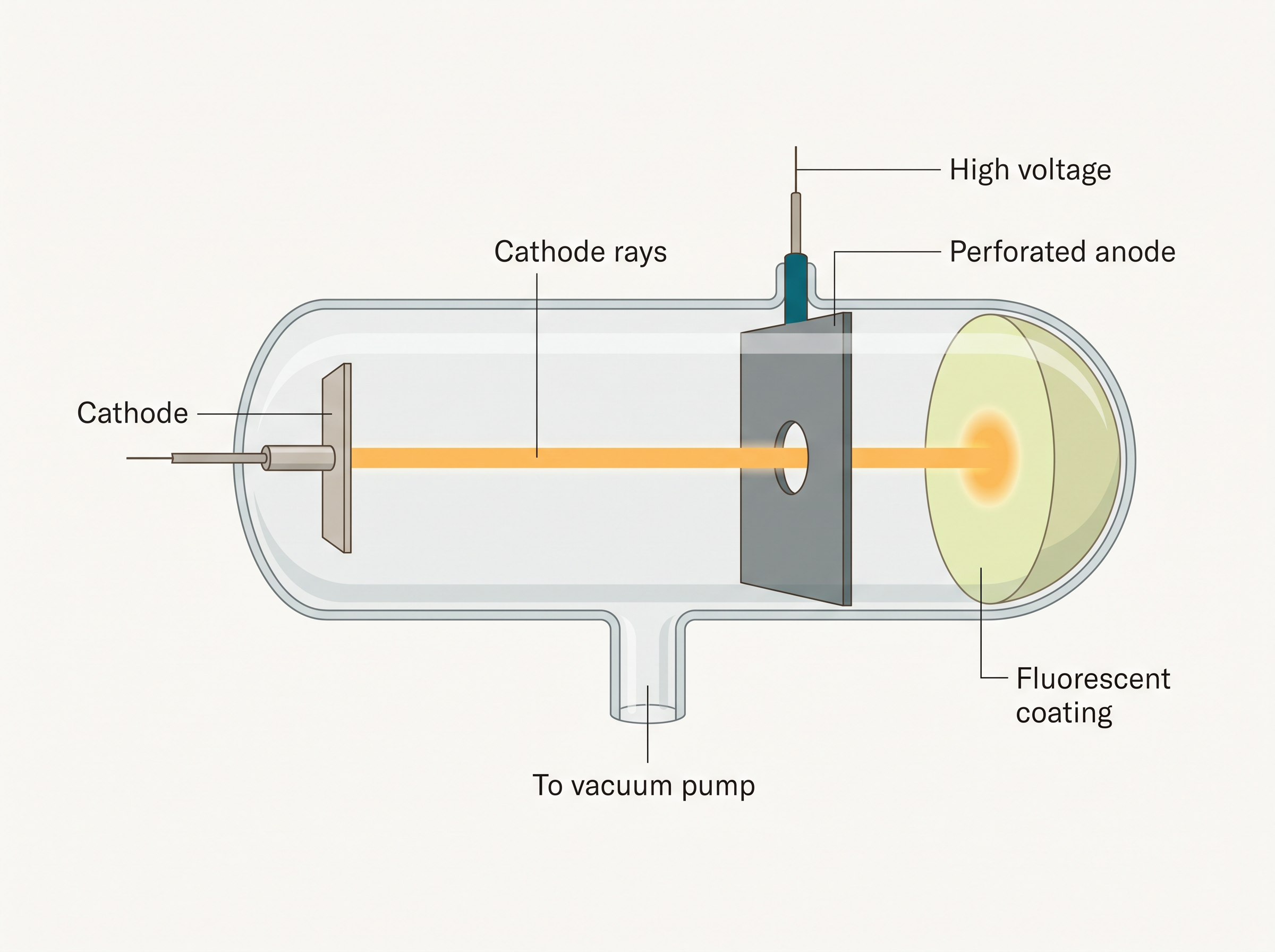
Fig. 2.2(b) – Cathode ray discharge tube with perforated anode.
The experiments on these tubes gave a set of clear results, which are worth listing carefully because each one tells us something about the nature of the rays.
First, the cathode rays start at the cathode and move towards the anode. Second, the rays themselves are invisible, but their arrival can be detected because certain materials — fluorescent or phosphorescent substances — glow when the rays hit them. This is exactly how old television picture tubes worked: they were cathode ray tubes, and the picture appeared because the screen was coated with materials that glowed when struck.
Third, in the absence of any electric or magnetic field, the rays travel in perfectly straight lines, as shown in Fig. 2.3. Fourth, when an electric or magnetic field is applied, the rays bend in exactly the way one would expect for negatively charged particles. This was the key clue: the cathode rays are made of negatively charged particles, and these particles are the electrons.
Fifth, and most important of all, the properties of these cathode rays do not depend on the material of the electrodes or on the kind of gas present in the tube. Whether the electrodes were made of one metal or another, whether the gas was hydrogen, oxygen, or anything else, the cathode ray particles came out exactly the same.
That last point carries a powerful conclusion. If every material and every gas gives the same negatively charged particle, then this particle must be present in all matter. In other words, electrons are a basic constituent of every atom.
2.1.2 Charge to Mass Ratio of Electron
Knowing that electrons exist is one thing; measuring them is another. In 1897, the British physicist J. J. Thomson designed a clever experiment to measure the ratio of the electron’s electric charge to its mass. This ratio is written \(e/m\_e\), where \(e\) is the magnitude of the charge and \(m\_e\) is the mass of the electron.
Thomson used a cathode ray tube fitted with both an electric field and a magnetic field, arranged perpendicular (at right angles) to each other and also perpendicular to the path of the electrons. The apparatus is shown in Fig. 2.3.
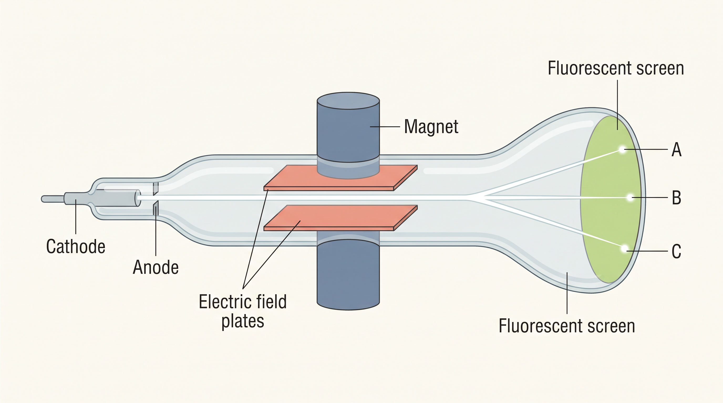
Fig. 2.3 – Thomson’s apparatus for measuring the charge-to-mass ratio.
The idea is to watch how far the electron beam is pushed off its straight path. When only the electric field is switched on, the electrons deviate and strike the tube at point A. When only the magnetic field is switched on, they strike at point C. By carefully adjusting the two field strengths against each other, the beam can be brought back to the undisturbed straight-line point B — the spot it would hit with no field at all.
Thomson reasoned that the amount by which the particles are pushed off their path depends on three things. First, the size of the negative charge on the particle: the greater the charge, the stronger its interaction with the field, and the greater the deflection. Second, the mass of the particle: a lighter particle is pushed aside more easily, so it deflects more. Third, the strength of the applied electric or magnetic field: raising the voltage across the electrodes, or increasing the magnetic field strength, increases the deflection.
By making accurate measurements of these deflections at known field strengths, Thomson was able to calculate the charge-to-mass ratio of the electron:
\[\\frac{e}{m\_e} = 1.758820 \\times 10^{11}\\ \\text{C kg}^{-1} \\qquad (2.1)\]
Here \(m\_e\) is the mass of the electron in kilograms and \(e\) is the magnitude of its charge in coulombs (C). Since the electron is negative, its actual charge is written as \(-e\).
2.1.3 Charge on the Electron
Thomson had found the ratio \(e/m\_e\), but not \(e\) and \(m\_e\) separately. To pin down the charge itself, R. A. Millikan (1868–1953) devised the famous oil drop experiment, carried out over the years 1906–1914.
Millikan found the charge on the electron to be about \(-1.6 \\times 10^{-19}\) C. The present accepted value is:
\[e = -1.602176 \\times 10^{-19}\\ \\text{C}\]
Once the charge \(e\) was known, the mass of the electron could be found by combining it with Thomson’s ratio from equation (2.1). We simply divide the charge by the charge-to-mass ratio:
\[m\_e = \\frac{e}{e/m\_e} = \\frac{1.602176 \\times 10^{-19}\\ \\text{C}}{1.758820 \\times 10^{11}\\ \\text{C kg}^{-1}}\]
\[m\_e = 9.1094 \\times 10^{-31}\\ \\text{kg} \\qquad (2.2)\]
Notice how a ratio plus one measured quantity gives us the second quantity — a common and useful trick in physics and chemistry.
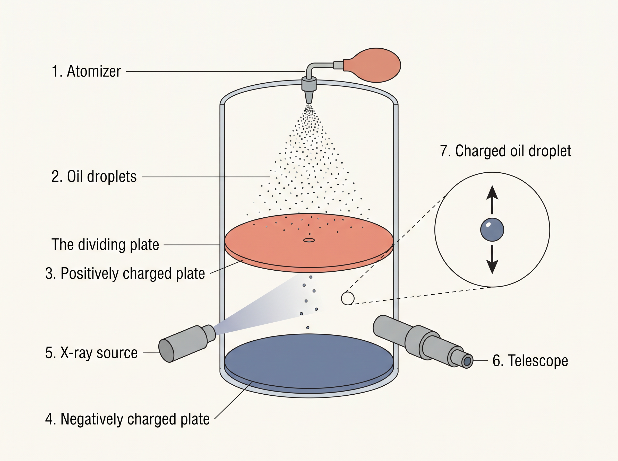
Fig. 2.4 – The Millikan oil drop apparatus.
2.1.4 Discovery of Protons and Neutrons
If atoms are neutral overall but contain negative electrons, they must also contain positive charge to balance them. The search for this positive charge again used a modified cathode ray tube. This time the experiment produced canal rays — rays carrying positively charged particles. Their behaviour was studied carefully and revealed several features.
First, unlike cathode rays, the mass of these positive particles depends on the nature of the gas present in the tube. They are simply the positively charged gaseous ions left behind when electrons are knocked off the gas atoms. Second, and for the same reason, the charge-to-mass ratio of these particles also changes with the gas used. Third, some of the positive particles carry a charge that is a whole-number multiple of the fundamental unit of charge. Fourth, in an electric or magnetic field these particles bend in the opposite direction to electrons — exactly what we expect, since they carry the opposite charge.
The smallest and lightest positive particle was produced when the gas in the tube was hydrogen. This particle was named the proton, and it was properly characterised in 1919. The proton carries a positive charge equal in size to the electron’s negative charge, but it is far heavier.
For a while, the atom seemed to be explained by just protons and electrons. But the masses did not add up. A need was felt for a third, electrically neutral particle inside the atom. These particles were finally discovered by James Chadwick in 1932. He bombarded a thin sheet of the element beryllium with α-particles (helium nuclei), and observed the emission of neutral particles whose mass was slightly greater than that of a proton. He named these particles neutrons.
With electrons, protons, and neutrons identified, the picture of the atom’s ingredients was complete. Their key properties are collected in Table 2.1. It is worth studying this table closely, because the whole of chemistry rests on these three particles and their arrangement.
Table 2.1 Properties of Fundamental Particles
| Name | Symbol | Absolute charge/C | Relative charge | Mass/kg | Mass/u | Approx. mass/u |
|---|---|---|---|---|---|---|
| Electron | e | \(-1.602176 \\times 10^{-19}\) | \(-1\) | \(9.109382 \\times 10^{-31}\) | 0.00054 | 0 |
| Proton | p | \(+1.602176 \\times 10^{-19}\) | \(+1\) | \(1.6726216 \\times 10^{-27}\) | 1.00727 | 1 |
| Neutron | n | 0 | 0 | \(1.674927 \\times 10^{-27}\) | 1.00867 | 1 |
Look carefully at the mass column. The proton and neutron are each nearly 1 u (unified atomic mass unit) and are almost 1800 times heavier than the electron, whose mass is so small it is taken as approximately 0 u. This single fact — that almost all of an atom’s mass sits in its protons and neutrons — will matter greatly when we discuss where the mass of an atom is concentrated.
2.2 Atomic Models
The experiments of the previous section overturned Dalton’s idea of an indivisible atom. We now knew that the atom is built from sub-atomic particles carrying positive and negative charges. But this raised a new set of questions that the discovery of the particles alone could not answer. Scientists now needed a model — a mental picture — of how these charged particles are arranged inside the atom.
Four big problems stood before them. They had to account for the stability of the atom (why it does not simply fly apart or collapse). They had to compare the behaviour of different elements in terms of both physical and chemical properties. They had to explain how different atoms combine to form the enormous variety of molecules. And they had to understand the origin and nature of the electromagnetic radiation that atoms absorb or give out.
To meet these challenges, several atomic models were proposed to describe how the charged particles are distributed within the atom. Some of these models could not explain the stability of atoms and were set aside. Two models, however, are important enough to study in detail: one put forward by J. J. Thomson, and the other by Ernest Rutherford.
2.2.1 Thomson Model of Atom
In 1898, J. J. Thomson proposed the first serious model of the internal atom. He suggested that an atom is a sphere (of radius about \(10^{-10}\) m) in which the positive charge is spread out uniformly, like a smooth positively charged jelly. The electrons are stuck into this positive sphere in the arrangement that gives the most stable, lowest-energy electrostatic balance, as shown in Fig. 2.5.
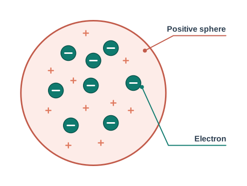
Fig. 2.5 – Thomson’s model of the atom.
This model has picked up several nicknames over the years — the plum pudding, raisin pudding, or watermelon model. The comparison is easy to picture: a pudding or watermelon of positive charge, studded with plums or seeds that stand for the electrons.
An important feature of Thomson’s model is that the mass of the atom is assumed to be spread evenly over the whole atom. This assumption will turn out to be exactly where the model fails.
Thomson’s model did succeed in one respect: it explained why an atom is electrically neutral overall, since the total negative charge of the embedded electrons balances the positive charge of the sphere. But it was not consistent with the results of later experiments, as we shall see in a moment. Thomson himself was awarded the Nobel Prize for Physics in 1906 for his theoretical and experimental work on the conduction of electricity by gases.
2.2.2 Rutherford’s Nuclear Model of Atom
The model that replaced Thomson’s came out of one of the most famous experiments in the history of science. Rutherford and his students Hans Geiger and Ernest Marsden carried out the α-particle scattering experiment, whose set-up is represented in Fig. 2.6.
A stream of high-energy α-particles from a radioactive source was aimed at a very thin foil of gold metal, about 100 nm thick. Around the foil was placed a circular screen coated with fluorescent zinc sulphide. Every time an α-particle struck this screen, it made a tiny flash of light, so the scientists could count where the particles went.
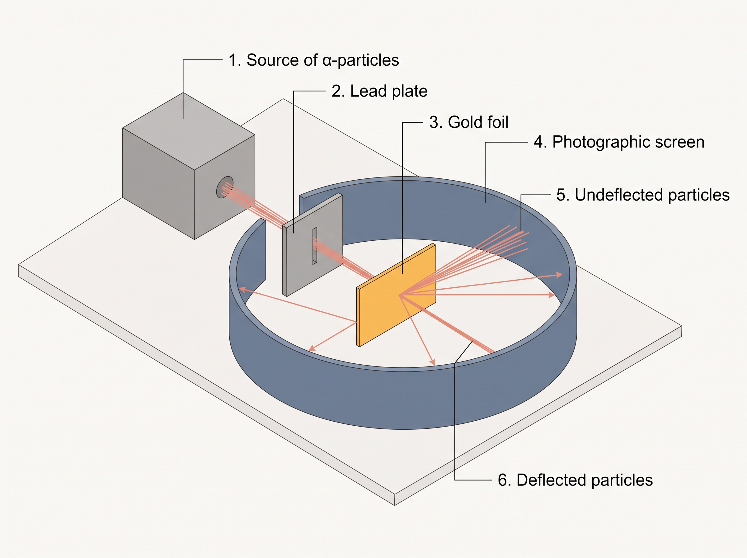
Fig. 2.6 – Rutherford’s alpha-particle scattering experiment.
Here is why the result was so shocking. If Thomson’s model were correct, the mass and positive charge of each gold atom would be spread evenly throughout it. The fast α-particles, carrying plenty of energy, should have sailed right through such a soft, uniform cloud of mass, slowing only slightly and changing direction by tiny angles at most. That is what everyone expected.
What actually happened was very different. Most of the α-particles did pass straight through the foil, undeflected. But a small fraction were deflected by small angles. And, most startling of all, a very few — about 1 in 20,000 — bounced almost straight back, deflected by nearly \(180°\). Rutherford later said this was as surprising as firing a shell at tissue paper and having it rebound at you.
From these observations, Rutherford drew a chain of conclusions about the structure of the atom. First, most of the space inside an atom is empty, because most α-particles passed through without any deflection. Second, the few particles that bounced back must have met an enormous repulsive force, which means the positive charge of the atom is not spread throughout it as Thomson had assumed, but is packed into a very tiny region — a region so concentrated it could repel and reverse a fast positive α-particle.
Third, calculations showed that this dense central region occupies almost no volume compared with the whole atom. The radius of an atom is about \(10^{-10}\) m, while the radius of this central region is only about \(10^{-15}\) m. To feel this difference, imagine that the central region were the size of a cricket ball — then the whole atom would be about 5 km across. The atom is overwhelmingly empty space with a tiny, heavy heart.
On the basis of these observations and conclusions, Rutherford proposed his nuclear model of the atom, which has three main features. The positive charge and nearly all the mass of the atom are densely packed into an extremely small central region, which Rutherford named the nucleus. The nucleus is surrounded by electrons that move around it at very high speed in circular paths called orbits; in this picture the atom resembles the solar system, with the nucleus playing the role of the sun and the electrons the role of the revolving planets. And the electrons and the nucleus are held together by the electrostatic force of attraction between opposite charges.
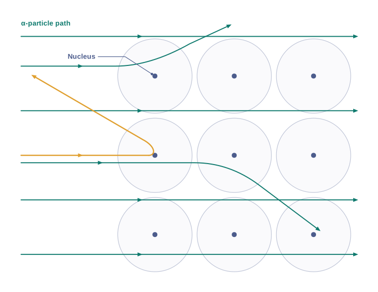
Fig. 2.7(b) – Schematic view of alpha particles scattering from gold nuclei.
2.2.3 Atomic Number and Mass Number
Now that the nucleus is in the picture, we can define two of the most important numbers in all of chemistry. The positive charge on the nucleus comes from the protons it contains. Since the proton’s charge is equal and opposite to the electron’s, the number of protons in the nucleus is called the atomic number and is given the symbol \(Z\).
For example, the hydrogen nucleus has 1 proton, so its atomic number is 1. The sodium nucleus has 11 protons, so its atomic number is 11. To keep the whole atom electrically neutral, the number of electrons must equal the number of protons. So a neutral hydrogen atom has 1 electron and a neutral sodium atom has 11 electrons.
\[Z = \\text{number of protons} = \\text{number of electrons (in a neutral atom)} \\qquad (2.3)\]
While the positive charge of the nucleus comes only from the protons, the mass of the nucleus comes from both the protons and the neutrons. Protons and neutrons together are collectively called nucleons. The total number of nucleons in an atom is called its mass number, given the symbol \(A\).
\[A = Z + n \\qquad (2.4)\]
This tidy pair of equations lets us find any one of the three quantities — protons, neutrons, electrons — as long as we know the other two, along with the charge on the species.
2.2.4 Isobars and Isotopes
Chemists use a compact shorthand to record the make-up of any atom. The element symbol X is written with the mass number \(A\) as a superscript and the atomic number \(Z\) as a subscript, both on the left-hand side, giving \(^A\_Z\\mathrm{X}\).
Two related terms describe how atoms can be similar in one number while differing in another. Isobars are atoms of different elements that have the same mass number \(A\) but different atomic numbers \(Z\). For example, \(^{14}*{\\ 6}\\mathrm{C}\) and \(^{14}*{\\ 7}\\mathrm{N}\) both have mass number 14, but their atomic numbers (6 and 7) differ, so they are isobars.
Isotopes, on the other hand, are atoms of the same element — same atomic number \(Z\) — but with different mass numbers \(A\). Looking at equation (2.4), we can see exactly what makes isotopes differ: since \(Z\) is the same, the difference in \(A\) must come from a different number of neutrons in the nucleus.
Hydrogen gives the clearest example of isotopes. About 99.985% of hydrogen atoms contain just one proton and no neutron; this isotope is called protium, \(^1\_1\\mathrm{H}\). A small fraction contains 1 proton and 1 neutron and is called deuterium, \(^2\_1\\mathrm{D}\) (about 0.015%). A third isotope, with 1 proton and 2 neutrons, is called tritium, \(^3\_1\\mathrm{T}\), and is found only in trace amounts on Earth.
Other common isotopes include carbon with 6, 7, and 8 neutrons besides its 6 protons — that is, \(^{12}*{\\ 6}\\mathrm{C}\), \(^{13}*{\\ 6}\\mathrm{C}\) and \(^{14}*{\\ 6}\\mathrm{C}\) — and chlorine with 18 and 20 neutrons besides its 17 protons — that is, \(^{35}*{17}\\mathrm{Cl}\) and \(^{37}\_{17}\\mathrm{Cl}\).
There is one more crucial point about isotopes. The chemical properties of an atom are controlled by its electrons, and the number of electrons is fixed by the number of protons. Neutrons have almost no effect on chemical behaviour. Therefore, all the isotopes of a given element show the same chemical behaviour — deuterium reacts just like ordinary protium, only more slowly and with slightly different physical properties owing to its greater mass.
A useful note before using the notation \(^A\_Z\\mathrm{X}\): first decide whether the species is a neutral atom, a cation, or an anion. If it is a neutral atom, equation (2.3) holds, so number of protons = number of electrons = atomic number. If it is an ion, check whether the protons outnumber the electrons (a cation, positive) or the electrons outnumber the protons (an anion, negative). The number of neutrons is always given by \(A - Z\), whether the species is neutral or an ion.
2.2.5 Drawbacks of Rutherford Model
Rutherford’s nuclear atom was a huge step forward, but it carried a fatal flaw. In this model, as we saw, the atom is a miniature solar system, with the heavy nucleus playing the part of the massive sun and the light electrons playing the part of the orbiting planets. To see why this comparison breaks down, we must look carefully at the difference between a planet and an electron.
When classical mechanics — the physics of Newton’s laws — is applied to the solar system, it correctly predicts that the planets move in stable, well-defined orbits around the sun. The gravitational force that holds a planet in orbit is given by the expression
\[F = G,\\frac{m\_1 m\_2}{r^2}\]
where \(m\_1\) and \(m\_2\) are the two masses, \(r\) is the distance between them, and \(G\) is the gravitational constant. This theory predicts the planetary orbits precisely, and its predictions match what astronomers actually observe.
The force between the electron and the nucleus looks mathematically very similar. It is the Coulomb force between two charges,
\[F = k,\\frac{q\_1 q\_2}{r^2}\]
where \(q\_1\) and \(q\_2\) are the charges, \(r\) is the distance between them, and \(k\) is a proportionality constant. Because the two force laws have the same form, it is tempting to conclude that the electron should orbit the nucleus in a stable path, just as a planet orbits the sun.
Here is where the analogy collapses. When any body moves in a circular orbit, it is constantly accelerating — even at constant speed — because its direction is always changing, and a change of direction is an acceleration. So an electron in a circular orbit is an accelerating charged particle. Now comes the crucial difference from a planet: according to Maxwell’s electromagnetic theory, an accelerating charged particle must continuously emit electromagnetic radiation. Planets are uncharged, so this does not affect them. But an orbiting electron is charged, so it must radiate energy away.
The energy carried off by this radiation comes from the electron’s own motion. As it loses energy, the electron cannot maintain its orbit — the orbit shrinks steadily inward. Calculations show that an electron should spiral into the nucleus in only about \(10^{-8}\) s. If Rutherford’s model were literally true, every atom would collapse in a hundred-millionth of a second. Clearly this does not happen, so the Rutherford model cannot explain the stability of the atom.
One might try to rescue the model by asking: if moving electrons make the atom unstable, why not simply let the electrons sit still? But this fails too. If the electrons were stationary, the electrostatic attraction between the dense positive nucleus and the electrons would immediately pull the electrons inward until they collapsed onto the nucleus — giving back, in effect, a tiny version of Thomson’s model. So neither a moving electron nor a stationary electron gives a stable atom in classical physics.
There is a second serious drawback as well. Rutherford’s model says nothing at all about how the electrons are arranged around the nucleus or what energies they have. It gives us a nucleus and some electrons, but no rules for the electrons’ distribution or energy. Yet, as we shall see, it is precisely this electronic arrangement that decides the chemistry of an element.
These two failures — the instability problem and the silence about electron arrangement — showed that a completely new kind of thinking was needed. The way forward came from studying how atoms interact with light, which is where the next section begins.
2.3 Developments Leading to the Bohr’s Model of Atom
The failures of the Rutherford model told scientists that a fresh approach was needed. That approach came from an unexpected direction: the study of how radiations — especially light — interact with matter. These studies gave immense information about the structure of atoms and molecules, and Niels Bohr used them to improve on Rutherford’s model.
Two developments, in particular, played a major role in shaping Bohr’s model. The first was the discovery that electromagnetic radiation has a dual character — it behaves in some experiments like a wave and in others like a stream of particles. The second was the set of experimental results on atomic spectra, the specific colours of light that atoms give out.
We will look first at the dual nature of electromagnetic radiation. The experimental results on atomic spectra are taken up later, in Section 2.4’s build-up (beginning in Section 2.3.3).
2.3.1 Wave Nature of Electromagnetic Radiation
In the mid-nineteenth century, physicists were busy studying how heated objects absorb and emit radiation. This radiation given off by hot bodies is called thermal radiation. Today we know that thermal radiation is made up of electromagnetic waves of many different frequencies or wavelengths. The theory of these waves was worked out in the early 1870s by James Clerk Maxwell, and it was confirmed experimentally later by Heinrich Hertz.
Maxwell (around 1870) was the first to give a full explanation of how charged bodies interact and how electric and magnetic fields behave on a large scale. He suggested that when an electrically charged particle moves with acceleration, it produces alternating electric and magnetic fields, and these fields spread outward as waves. These are called electromagnetic waves or electromagnetic radiation.
Light itself is one form of such radiation, and ideas about its nature go back a long way. In earlier times (Newton’s era) light was thought to be made of tiny particles called corpuscles. It was only in the nineteenth century that the wave nature of light was firmly established. Maxwell then showed that light waves are associated with oscillating electric and magnetic character, as pictured in Fig. 2.8.

Fig. 2.8 – The electric and magnetic field components of an electromagnetic wave.
Although electromagnetic wave motion is complicated, a few simple properties are enough for our purpose. First, the oscillating electric and magnetic fields produced by an oscillating charged particle are perpendicular to each other, and both are perpendicular to the direction in which the wave travels (Fig. 2.8). Second, unlike sound waves or water waves, electromagnetic waves do not need any medium to travel through — they can move through a vacuum.
Third, there are many different types of electromagnetic radiation, differing from one another in wavelength or frequency. Together they make up what is called the electromagnetic spectrum (Fig. 2.9). Different regions of this spectrum have different names and uses: the radio-frequency region around \(10^6\) Hz is used for broadcasting; the microwave region around \(10^{10}\) Hz is used for radar; the infrared region around \(10^{13}\) Hz is used for heating; and the ultraviolet region around \(10^{16}\) Hz is a component of sunlight. The small portion around \(10^{15}\) Hz is ordinarily called visible light — this is the only part our eyes can detect, and special instruments are needed to detect the rest.
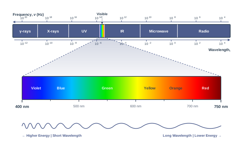
Fig. 2.9 – The electromagnetic spectrum and the visible region.
Fourth, different kinds of units are used to describe electromagnetic radiation. These radiations are characterised by two main properties: frequency (symbol \(\\nu\)) and wavelength (symbol \(\\lambda\)).
The SI unit of frequency \(\\nu\) is the hertz (Hz, or \(\\text{s}^{-1}\)), named after Heinrich Hertz. Frequency is defined as the number of waves that pass a given point in one second.
Wavelength should have units of length, and the SI unit of length is the metre (m). Because electromagnetic radiation comes in many kinds with much smaller wavelengths, smaller units are often used. Figure 2.9 shows the various types of electromagnetic radiation, which differ in wavelength and frequency.
A key fact ties these together. In a vacuum, all types of electromagnetic radiation, whatever their wavelength, travel at exactly the same speed: \(3.0 \\times 10^8\\ \\text{m s}^{-1}\) (more precisely \(2.997925 \\times 10^8\\ \\text{m s}^{-1}\)). This is the speed of light, given the symbol \(c\). The frequency \(\\nu\), wavelength \(\\lambda\), and speed of light \(c\) are related by a simple and very important equation:
\[c = \\nu\\lambda \\qquad (2.5)\]
This tells us that frequency and wavelength are inversely related for light: a longer wavelength means a lower frequency, and a shorter wavelength means a higher frequency.
The wavenumber
There is one more quantity used often in spectroscopy: the wavenumber, written \(\\bar{\\nu}\). It is defined as the number of wavelengths per unit length. Its unit is the reciprocal of the wavelength unit — that is, \(\\text{m}^{-1}\) — although the more commonly used unit is \(\\text{cm}^{-1}\) (which is not an SI unit). Since it is the reciprocal of wavelength, \(\\bar{\\nu} = 1/\\lambda\).
2.3.2 Particle Nature of Electromagnetic Radiation: Planck’s Quantum Theory
The wave picture of light explained some phenomena beautifully — for example diffraction (the bending of a wave around an obstacle) and interference (the combining of two waves, where their disturbances add up or cancel out at each point). But there were several observations that even the electromagnetic wave theory of nineteenth-century physics (called classical physics) could not explain. These were the awkward facts that forced a whole new idea onto physics.
Four such observations stood out. First, the nature of the radiation emitted by hot bodies (black-body radiation). Second, the ejection of electrons from a metal surface when radiation strikes it (the photoelectric effect). Third, the way the heat capacity of solids changes with temperature. And fourth, the line spectra of atoms, especially the spectrum of hydrogen.
The common thread running through all these phenomena is that the system can take up or give out energy only in fixed, discrete amounts — not in any amount you please. Energy, it seemed, comes in packets.
Black-body radiation and the birth of the quantum
The first solid explanation of black-body radiation was given by Max Planck in 1900. To understand what he explained, we first need to understand the phenomenon itself.
Hot objects give out electromagnetic radiation over a wide range of wavelengths. At high temperatures, a large share of this radiation lies in the visible region. As the temperature rises, more of the radiation shifts to shorter wavelengths (towards blue light). A familiar example is an iron rod heated in a furnace: it first turns dull red, then grows brighter and redder, then becomes white, and finally, at very high temperatures, glows blue. This shows that the intensities of different wavelengths given out by a hot body depend on its temperature.
By the late 1850s it was known that objects made of different materials, kept at different temperatures, give out different amounts of radiation. Also, when light falls on an object, part of the radiant energy is reflected, part is absorbed, and part is transmitted. Ordinary objects are imperfect absorbers, which is why absorption is incomplete.
To study this cleanly, physicists imagined an ideal object. An ideal body that emits and absorbs radiation of all frequencies uniformly is called a black body, and the radiation emitted by such a body is called black-body radiation. In practice no perfect black body exists, but carbon black comes fairly close, and a good practical black body is a cavity with a tiny hole and no other opening: any ray entering the hole bounces around inside and is eventually absorbed by the walls.
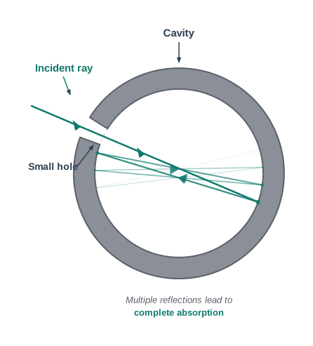
Fig. 2.10(a) – A cavity model of a black body.
A black body is also a perfect radiator of energy, and it stays in thermal equilibrium with its surroundings, giving out as much energy per unit area as it absorbs. The amount and spread of the light it emits depend only on its temperature. At a given temperature, the intensity of emitted radiation rises with wavelength, reaches a maximum at a particular wavelength, and then falls off again as wavelength increases further, as shown in Fig. 2.11. As the temperature rises, the peak of the curve shifts to shorter wavelengths.
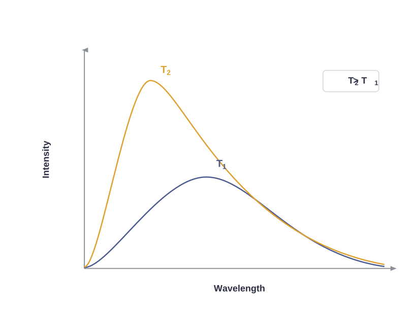
Fig. 2.11 – Black-body radiation intensity versus wavelength.
Many attempts were made to predict the intensity of black-body radiation as a function of wavelength using the wave theory of light, and all of them failed to match the experiment. Max Planck finally arrived at a relationship that worked, but only by making a bold assumption. He proposed that the absorption and emission of radiation arise from the oscillators — the atoms in the walls of the black body — whose frequency of oscillation can change through interaction with the radiation. Crucially, Planck assumed that radiation could be sub-divided only into discrete chunks of energy. Atoms and molecules, he said, can emit or absorb energy only in discrete quantities, not continuously.
He gave the name quantum to the smallest quantity of energy that can be emitted or absorbed as electromagnetic radiation. The energy \(E\) of one quantum of radiation is proportional to its frequency \(\\nu\), and this is expressed by Planck’s equation:
\[E = h\\nu \\qquad (2.6)\]
The proportionality constant \(h\) is called Planck’s constant and has the value \(6.626 \\times 10^{-34}\\ \\text{J s}\). This tiny number is one of the most important constants in all of science.
With this theory, Planck could correctly explain how the intensity of black-body radiation varies with frequency (or wavelength) at different temperatures.
A helpful way to picture quantisation is a staircase. A person can stand on any step of a staircase, but not in between two steps — there is no halfway position. In the same way, the energy of a quantum system can take only one of a fixed set of values, and nothing in between:
\[E = 0,\\ h\\nu,\\ 2h\\nu,\\ 3h\\nu, \\ldots, nh\\nu, \\ldots\]
The photoelectric effect
In 1887, H. Hertz performed a striking experiment: when certain metals (such as potassium, rubidium, and caesium) were exposed to a beam of light, electrons were ejected from the metal surface. This is the photoelectric effect, and the set-up is shown in Fig. 2.12.
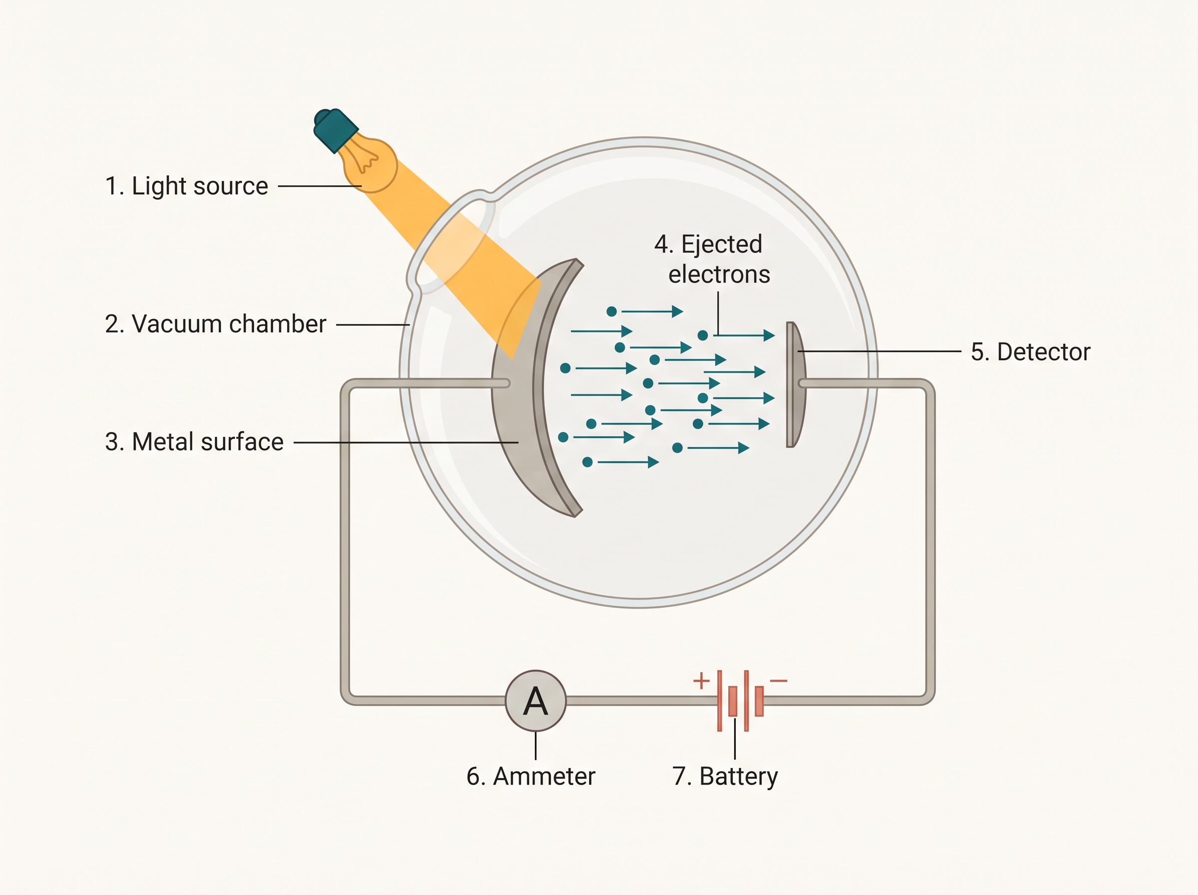
Fig. 2.12 – Equipment for studying the photoelectric effect.
Three results of this experiment must be explained. First, electrons are ejected from the metal the instant the light beam strikes it — there is no time lag at all between the light hitting the surface and the electrons flying off. Second, the number of electrons ejected is proportional to the intensity (brightness) of the light. Third, for each metal there is a characteristic minimum frequency \(\\nu\_0\), called the threshold frequency, below which no electrons are ejected however bright the light. Above this frequency (\(\\nu > \\nu\_0\)) the ejected electrons come out with kinetic energy, and this kinetic energy increases as the frequency of the light increases.
None of this could be explained by classical physics. Classically, the energy of a light beam depends on its brightness, so both the number of ejected electrons and their kinetic energy should depend on brightness. But experiment showed the opposite for kinetic energy. For example, red light with \(\\nu = (4.3\\text{ to }4.6) \\times 10^{14}\) Hz, no matter how bright, could shine on potassium for hours and eject no electrons at all. Yet even a very weak yellow light with \(\\nu = 5.1\\text{–}5.2 \\times 10^{14}\) Hz ejected electrons at once. The threshold frequency \(\\nu\_0\) for potassium is \(5.0 \\times 10^{14}\) Hz.
Einstein solved this puzzle in 1905, using Planck’s quantum theory as his starting point. His idea was that a beam of light is a stream of energy packets called photons, each of energy \(h\\nu\). Shining light on a metal is like firing a beam of these photons at it. When a photon of sufficient energy strikes an electron in the metal atom, it transfers all its energy to that electron in a single collision, and the electron is knocked out instantly — with no time lag. This immediately explains the “no delay” result and the threshold: a photon below the threshold frequency simply does not carry enough energy to free an electron, no matter how many such photons arrive.
The greater the energy of the photon, the more energy is handed to the electron, and the greater its kinetic energy on ejection. So the kinetic energy of the ejected electron is proportional to the frequency of the light, not its brightness.
We can turn this into an energy equation. The striking photon has energy \(h\\nu\). The minimum energy needed to eject the electron is \(h\\nu\_0\), which is also called the work function, \(W\_0\) (values for a few metals are given in Table 2.2). By the conservation of energy, whatever energy is left over after freeing the electron appears as the electron’s kinetic energy:
\[h\\nu = h\\nu\_0 + \\frac{1}{2}m\_e v^2 \\qquad (2.7)\]
Here \(m\_e\) is the mass of the electron and \(v\) is the velocity of the ejected electron. Rearranged, the kinetic energy of the photoelectron is \(\\frac{1}{2}m\_e v^2 = h\\nu - h\\nu\_0 = h(\\nu - \\nu\_0)\).
Table 2.2 Values of Work Function (\(W\_0\)) for a Few Metals
| Metal | Li | Na | K | Mg | Cu | Ag |
|---|---|---|---|---|---|---|
| \(W\_0\) /eV | 2.42 | 2.3 | 2.25 | 3.7 | 4.8 | 4.3 |
Finally, why does a brighter beam eject more electrons? Because a more intense beam simply contains more photons. More photons mean more collisions and therefore more ejected electrons — but each individual electron’s kinetic energy still depends only on the frequency of the light.
Dual Behaviour of Electromagnetic Radiation
The photoelectric effect and black-body radiation forced scientists into a genuine dilemma. On the one hand, treating light as a stream of particles (photons) explained both of these beautifully. On the other hand, this particle picture clashed with the well-established wave behaviour of light, which was needed to explain interference and diffraction.
The only way out was to accept a surprising idea: light possesses both particle-like and wave-like properties — light has dual behaviour. Depending on the experiment, light behaves either as a wave or as a stream of particles. Whenever radiation interacts with matter (as in the photoelectric effect), it shows its particle-like side; whenever it propagates through space (as in interference and diffraction), it shows its wave-like side.
This concept was completely alien to how scientists had thought about matter and radiation, and it took a long time for them to accept it. As we shall see later, some tiny particles of matter — such as electrons — also turn out to show this same wave–particle duality.
2.3.3 Evidence for the Quantized Electronic Energy Levels: Atomic Spectra
We now come to the second great clue behind Bohr’s model: the spectra of atoms. The word quantized means the restriction of any property to a set of discrete values.
The speed of light depends on the medium it travels through. As a result, a beam of light is bent (refracted) when it passes from one medium to another. When a ray of white light passes through a prism, the shorter-wavelength waves bend more than the longer-wavelength ones. Because ordinary white light contains all the wavelengths of the visible range, it spreads out into a series of coloured bands called a spectrum. Red light, with the longest wavelength, is bent the least; violet light, with the shortest wavelength, is bent the most.
The visible spectrum we can see ranges from violet at \(7.50 \\times 10^{14}\) Hz to red at \(4 \\times 10^{14}\) Hz. Such a spectrum is called a continuous spectrum — “continuous” because the colours merge smoothly into one another, violet into blue, blue into green, and so on. A rainbow is a natural example of a continuous spectrum. Remember, though, that visible light is only a small part of the whole electromagnetic radiation (Fig. 2.9).
When electromagnetic radiation interacts with matter, atoms and molecules may absorb energy and jump to a higher energy state. In this higher state they are unstable, so to return to their normal, more stable, lower-energy state, they emit radiation in various regions of the electromagnetic spectrum. This absorbing and emitting of radiation is the origin of atomic spectra.
Emission and Absorption Spectra
The spectrum of radiation emitted by a substance that has absorbed energy is called an emission spectrum. Atoms, molecules, or ions that have absorbed radiation are said to be “excited.” To produce an emission spectrum, energy is supplied to a sample (by heating or irradiating it), and the wavelength of the radiation the sample gives out, as it releases the absorbed energy, is recorded.
An absorption spectrum is like the photographic negative of an emission spectrum. Here, a continuous stream of radiation is passed through a sample, which absorbs radiation of certain wavelengths. The missing wavelengths — those absorbed by the sample — show up as dark spaces in an otherwise bright continuous spectrum.
The study of emission or absorption spectra is called spectroscopy. The visible spectrum discussed above was continuous, because all wavelengths from red to violet are present. But the emission spectra of atoms in the gas phase are strikingly different: they do not show a continuous spread of colour. Instead, atoms emit light only at certain specific wavelengths, with dark gaps in between. Such spectra are called line spectra or atomic spectra, because the emitted radiation shows up as a pattern of bright lines (Fig. 2.13).
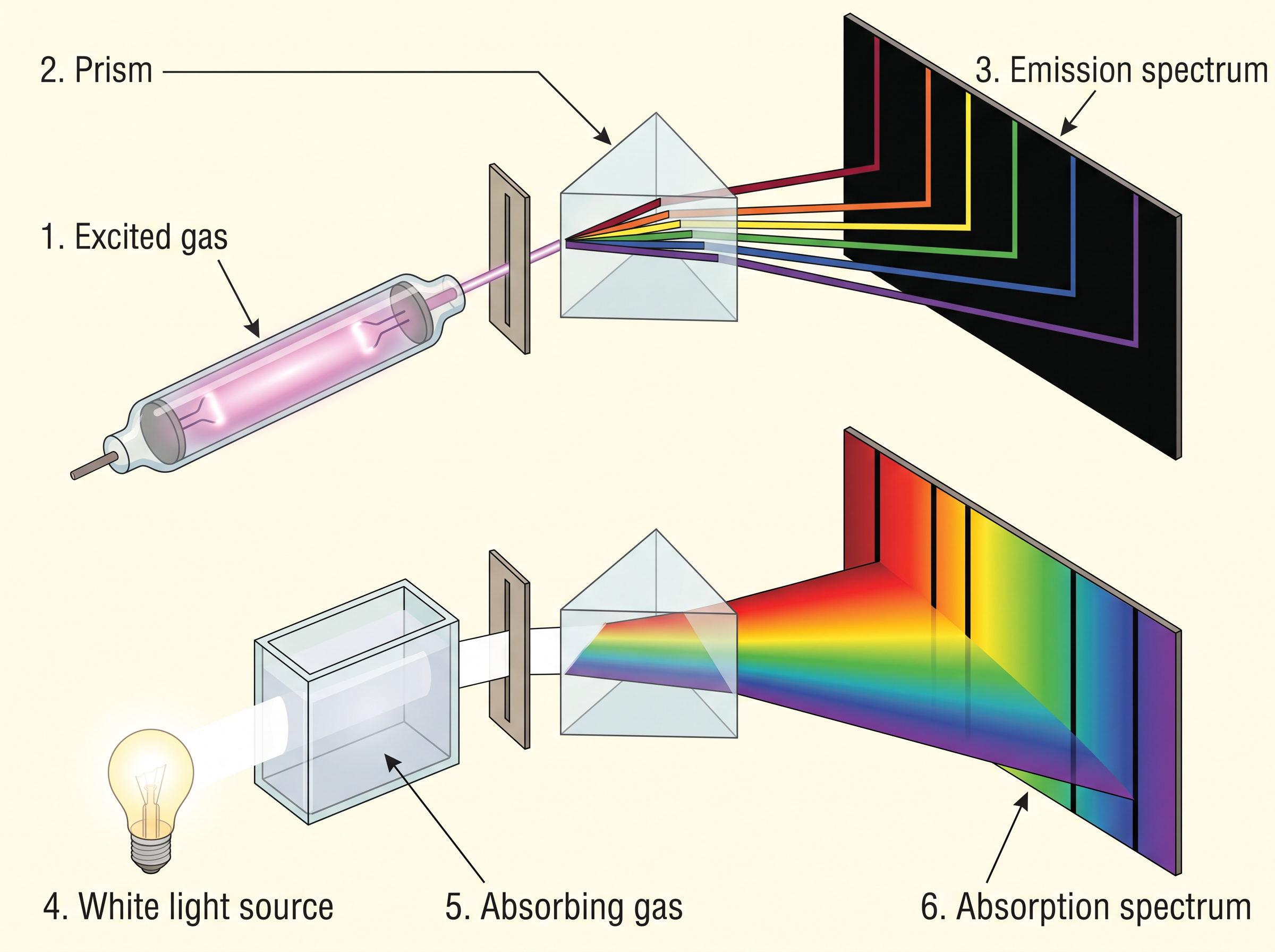
Fig. 2.13 – Atomic emission and absorption spectra.
Line emission spectra are of great interest for the study of electronic structure, because each element has a unique line emission spectrum. The characteristic lines of an atom act like a fingerprint: they can be used to identify unknown atoms, just as fingerprints identify people. Matching the emission lines of an unknown sample against those of a known element quickly reveals its identity. The German chemist Robert Bunsen (1811–1899) was among the first to use line spectra to identify elements.
Line Spectrum of Hydrogen
Hydrogen provides the simplest and most studied line spectrum. When an electric discharge is passed through gaseous hydrogen, the \(\\mathrm{H\_2}\) molecules split apart, and the excited hydrogen atoms produced emit electromagnetic radiation of discrete frequencies. The hydrogen spectrum consists of several series of lines, each named after its discoverer.
In 1885, Balmer showed, from experimental observations, that if the spectral lines are expressed in terms of wavenumber \(\\bar{\\nu}\), the visible lines of the hydrogen spectrum obey a simple formula:
\[\\bar{\\nu} = 109{,}677 \\left( \\frac{1}{2^2} - \\frac{1}{n^2} \\right)\\ \\text{cm}^{-1} \\qquad (2.8)\]
where \(n\) is an integer equal to or greater than 3 (that is, \(n = 3, 4, 5, \\ldots\)). The lines described by this formula are called the Balmer series, and they are the only lines of the hydrogen spectrum that appear in the visible region.
The Swedish spectroscopist Johannes Rydberg then noticed that all the series of lines in the hydrogen spectrum could be described by one more general expression:
\[\\bar{\\nu} = 109{,}677 \\left( \\frac{1}{n\_1^2} - \\frac{1}{n\_2^2} \\right)\\ \\text{cm}^{-1} \\qquad (2.9)\]
where \(n\_1 = 1, 2, \\ldots\) and \(n\_2 = n\_1 + 1,\\ n\_1 + 2, \\ldots\)
The value \(109{,}677\\ \\text{cm}^{-1}\) is called the Rydberg constant for hydrogen. The first five series of lines, corresponding to \(n\_1 = 1, 2, 3, 4, 5\), are known as the Lyman, Balmer, Paschen, Brackett, and Pfund series respectively. Table 2.3 lists these series, and Fig. 2.14 shows the Lyman, Balmer, and Paschen series of transitions for the hydrogen atom.
Table 2.3 The Spectral Lines for Atomic Hydrogen
| Series | \(n\_1\) | \(n\_2\) | Spectral Region |
|---|---|---|---|
| Lyman | 1 | 2, 3, … | Ultraviolet |
| Balmer | 2 | 3, 4, … | Visible |
| Paschen | 3 | 4, 5, … | Infrared |
| Brackett | 4 | 5, 6, … | Infrared |
| Pfund | 5 | 6, 7, … | Infrared |
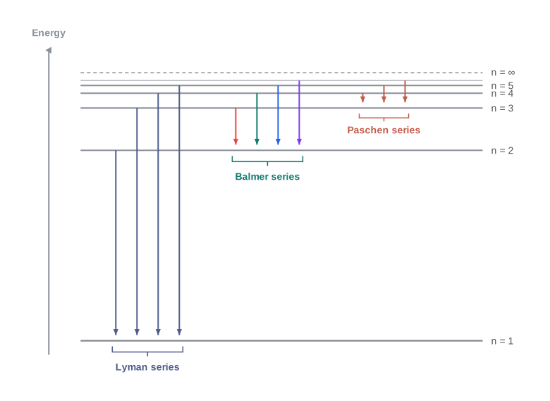
Fig. 2.14 – Energy-level diagram and spectral transitions for the hydrogen atom.
Of all the elements, hydrogen has the simplest line spectrum, and the spectrum becomes more and more complex for heavier atoms. Even so, all line spectra share two features: the line spectrum of each element is unique, and there is a regularity in the pattern of lines for each element. These similarities raise deep questions — what causes them, and are they connected to the electronic structure of atoms? As we shall find, the answers to these questions are exactly the key to understanding the electronic structure of the elements, and they lead us straight to Bohr’s model in the next section.
2.4 Bohr’s Model for Hydrogen Atom
Niels Bohr (1913) was the first to explain, in a quantitative way, the general features of the hydrogen atom’s structure and its spectrum. He built his model on Planck’s idea that energy is quantised. Bohr’s theory is not the full modern quantum mechanics, but it is still remarkably useful for making sense of many features of atomic structure and spectra. The whole model rests on a set of postulates — starting assumptions that Bohr made and then tested against experiment.
The postulates of Bohr’s model
Bohr’s model for the hydrogen atom is based on the following postulates.
The first postulate is that the electron in the hydrogen atom moves around the nucleus only in certain circular paths of fixed radius and energy. These allowed paths are called orbits, stationary states, or allowed energy states, and they are arranged concentrically (one inside another) around the nucleus. This is Bohr’s boldest step: unlike a planet, which could in principle orbit at any distance, the electron is allowed only in these special orbits.
The second postulate is that the energy of an electron in a given orbit does not change with time. As long as the electron stays in an orbit, it neither gains nor loses energy — this is why the orbits are called “stationary states.” The electron changes its energy only by jumping between orbits: it moves from a lower orbit to a higher one when it absorbs exactly the right amount of energy, and it moves from a higher orbit to a lower one by emitting energy. This jump is sudden, not gradual — the energy change does not happen in a continuous manner.
Here it helps to recall what angular momentum means, since Bohr’s next postulate uses it. Just as ordinary (linear) momentum is the product of mass (\(m\)) and linear velocity (\(v\)), angular momentum is the product of the moment of inertia (\(I\)) and the angular velocity (\(\\omega\)). For an electron of mass \(m\_e\) moving in a circular path of radius \(r\) around the nucleus, angular momentum \(= I \\times \\omega\). Since \(I = m\_e r^2\) and \(\\omega = v/r\) (where \(v\) is the linear velocity), we get angular momentum \(= m\_e r^2 \\times (v/r) = m\_e v r\).
The third postulate is Bohr’s frequency rule. When an electron jumps between two stationary states differing in energy by \(\\Delta E\), the frequency \(\\nu\) of the radiation absorbed or emitted is given by:
\[\\nu = \\frac{\\Delta E}{h} = \\frac{E\_2 - E\_1}{h} \\qquad (2.10)\]
where \(E\_1\) and \(E\_2\) are the energies of the lower and higher allowed states, respectively. This is commonly called Bohr’s frequency rule.
The fourth postulate is that the angular momentum of the electron is quantised — it cannot take just any value. In a given stationary state, it must be a whole-number multiple of \(h/2\\pi\):
\[m\_e v r = n \\cdot \\frac{h}{2\\pi}, \\qquad n = 1, 2, 3, \\ldots \\qquad (2.11)\]
where \(m\_e\) is the mass of the electron, \(v\) its velocity, and \(r\) the radius of the orbit.
This postulate is what makes Bohr’s model different in spirit from classical physics. An electron can move only in orbits where its angular momentum is an integral multiple of \(h/2\\pi\) — no other orbits are allowed. Radiation is absorbed or emitted only when the electron jumps from one such quantised orbit to another. Because of this, Maxwell’s electromagnetic theory (which demanded that an orbiting electron continuously radiate) simply does not apply within an allowed orbit — and that is precisely why only certain fixed orbits are stable, resolving the collapse problem that had doomed Rutherford’s model.
Results of Bohr’s theory
The full derivation of the energies of the stationary states is complicated and is left for higher classes, but Bohr’s theory for the hydrogen atom gives several important results that we can use directly.
First, the stationary states are numbered \(n = 1, 2, 3, \\ldots\) These whole numbers are called principal quantum numbers.
Second, the radii of the stationary states are given by:
\[r\_n = n^2 a\_0 \\qquad (2.12)\]
where \(a\_0 = 52.9\) pm. So the radius of the first stationary state, called the Bohr orbit, is 52.9 pm. Normally the electron in a hydrogen atom is found in this first orbit (\(n = 1\)). As \(n\) increases, \(r\) increases, meaning the electron is found further from the nucleus.
Third, and most important, is the energy of each stationary state, given by:
\[E\_n = -R\_H \\left( \\frac{1}{n^2} \\right), \\qquad n = 1, 2, 3, \\ldots \\qquad (2.13)\]
where \(R\_H\) is the Rydberg constant with the value \(2.18 \\times 10^{-18}\) J. The energy of the lowest state, the ground state, is found by putting \(n = 1\):
\[E\_1 = -2.18 \\times 10^{-18}\\left(\\frac{1}{1^2}\\right) = -2.18 \\times 10^{-18}\\ \\text{J}\]
The energy of the state \(n = 2\) is:
\[E\_2 = -2.18 \\times 10^{-18}\\left(\\frac{1}{2^2}\\right) = -0.545 \\times 10^{-18}\\ \\text{J}\]
Figure 2.14 (introduced in the previous section) depicts these energy levels; such a picture is called an energy level diagram.
What the negative sign means
Students often find the negative sign in equation (2.13) confusing, so it is worth pausing on it. When the electron is completely free of the nucleus’s influence, its energy is taken as zero; this corresponds to \(n = \\infty\) and is called the ionised hydrogen atom. When the electron is drawn in by the nucleus and settles into an orbit \(n\), energy is released, so the electron’s energy becomes lower than zero — that is, negative.
A free electron at rest, infinitely far from the nucleus, is assigned zero energy. Setting \(n = \\infty\) in equation (2.13) gives \(E\_\\infty = 0\), agreeing with this. As the electron moves closer to the nucleus (\(n\) decreases), \(E\_n\) becomes larger in size but more and more negative. The most negative energy, corresponding to \(n = 1\), is the most stable state — the ground state. So the negative sign simply tells us that a bound electron has lower energy than a free one, and the more negative the energy, the more tightly bound and stable the electron is.
Bohr’s model for hydrogen-like ions
Bohr’s theory is not limited to hydrogen. It also works for any ion that contains only one electron — species like \(\\mathrm{He^+}\), \(\\mathrm{Li^{2+}}\), \(\\mathrm{Be^{3+}}\), and so on. These are called hydrogen-like species. For them, the energies of the stationary states are given by:
\[E\_n = -2.18 \\times 10^{-18}\\left(\\frac{Z^2}{n^2}\\right)\\ \\text{J} \\qquad (2.14)\]
and the radii by:
\[r\_n = \\frac{52.9,(n^2)}{Z}\\ \\text{pm} \\qquad (2.15)\]
where \(Z\) is the atomic number, which has values 2 and 3 for helium and lithium respectively. From these equations we can see that as \(Z\) increases, the energy becomes more negative and the radius becomes smaller. This means the electron is more tightly bound to the nucleus in a hydrogen-like ion with a larger nuclear charge — which makes sense, since a bigger positive charge pulls the single electron in harder.
Finally, it is also possible to calculate the velocities of electrons in these orbits. Although the exact equation is not given here, qualitatively the velocity of the electron increases as the positive charge on the nucleus increases, and decreases as the principal quantum number increases.
2.4.1 Explanation of Line Spectrum of Hydrogen
Bohr’s model does something the earlier models could not: it explains the line spectrum of hydrogen quantitatively. Recall from Section 2.3.3 that hydrogen emits light only at certain fixed wavelengths. Bohr’s postulates tell us exactly why.
According to the second postulate, radiation is absorbed when the electron jumps from a lower-energy orbit (smaller principal quantum number) to a higher-energy orbit (larger principal quantum number), and radiation is emitted when the electron falls from a higher orbit to a lower one. The energy gap between the two orbits is:
\[\\Delta E = E\_f - E\_i \\qquad (2.16)\]
Combining equations (2.13) and (2.16), and letting \(n\_i\) and \(n\_f\) stand for the initial and final orbits:
\[\\Delta E = \\left(-\\frac{R\_H}{n\_f^2}\\right) - \\left(-\\frac{R\_H}{n\_i^2}\\right)\]
\[\\Delta E = R\_H \\left( \\frac{1}{n\_i^2} - \\frac{1}{n\_f^2} \\right) = 2.18 \\times 10^{-18}\\ \\text{J} \\left( \\frac{1}{n\_i^2} - \\frac{1}{n\_f^2} \\right) \\qquad (2.17)\]
The frequency \(\\nu\) associated with the absorption or emission of the photon can then be found using equation (2.18), dividing the energy gap by Planck’s constant:
\[\\nu = \\frac{\\Delta E}{h} = \\frac{R\_H}{h}\\left( \\frac{1}{n\_i^2} - \\frac{1}{n\_f^2} \\right)\]
\[\\nu = \\frac{2.18 \\times 10^{-18}\\ \\text{J}}{6.626 \\times 10^{-34}\\ \\text{J s}}\\left( \\frac{1}{n\_i^2} - \\frac{1}{n\_f^2} \\right) \\qquad (2.18)\]
\[\\nu = 3.29 \\times 10^{15}\\left( \\frac{1}{n\_i^2} - \\frac{1}{n\_f^2} \\right)\\ \\text{Hz} \\qquad (2.19)\]
The same relation can be written in terms of wavenumber \(\\bar{\\nu}\) by dividing the frequency by the speed of light \(c\):
\[\\bar{\\nu} = \\frac{\\nu}{c} = \\frac{R\_H}{hc}\\left( \\frac{1}{n\_i^2} - \\frac{1}{n\_f^2} \\right) \\qquad (2.20)\]
\[\\bar{\\nu} = \\frac{3.29 \\times 10^{15}\\ \\text{s}^{-1}}{3 \\times 10^8\\ \\text{m s}^{-1}}\\left( \\frac{1}{n\_i^2} - \\frac{1}{n\_f^2} \\right) = 1.09677 \\times 10^7 \\left( \\frac{1}{n\_i^2} - \\frac{1}{n\_f^2} \\right)\\ \\text{m}^{-1} \\qquad (2.21)\]
We can now read off which lines are absorption and which are emission. In an absorption spectrum, \(n\_f > n\_i\): the electron climbs to a higher orbit, the term in the bracket is positive, and energy is absorbed. In an emission spectrum, \(n\_i > n\_f\): the electron drops to a lower orbit, \(\\Delta E\) is negative, and energy is released.
Notice that expression (2.17) has exactly the same form as the one Rydberg had found empirically (equation 2.9), which he had obtained just by fitting experimental data. Bohr’s achievement was to derive this pattern from a physical model rather than merely fit it. Furthermore, each spectral line, whether in absorption or emission, can now be linked to a specific electron transition in the hydrogen atom. In a large collection of hydrogen atoms, many different transitions occur at once, giving the many observed spectral lines. The brightness (intensity) of a line depends on the number of photons of that wavelength being absorbed or emitted.
Flowchart
FC 2.14 – Origin of a hydrogen spectral line: electron absorbs energy → jumps from lower orbit nᵢ to higher orbit nₑ (excited state, unstable) → falls back from higher orbit to lower orbit → emits a photon of energy ΔE = R_H(1/n_f² − 1/n_i²) → one bright line appears in the spectrum; branch by final orbit: fall to n=1 → Lyman (UV); fall to n=2 → Balmer (visible); fall to n=3 → Paschen (IR).
2.4.2 Limitations of Bohr’s Model
Bohr’s model was a genuine triumph — it explained the stability and the line spectra of hydrogen and of hydrogen-like ions such as \(\\mathrm{He^+}\), \(\\mathrm{Li^{2+}}\), and \(\\mathrm{Be^{3+}}\). Yet it was too simple to account for several other observations, and understanding its failures points the way to the modern quantum theory.
First, Bohr’s model fails to explain the finer details of the hydrogen spectrum. Using sophisticated spectroscopic techniques, each spectral line was found to be split into closely spaced lines (for example, doublets). Bohr’s model has no explanation for this splitting. It is also unable to explain the spectrum of any atom with more than one electron — even helium, with just two electrons, is beyond it. Furthermore, Bohr’s theory cannot explain the splitting of spectral lines in a magnetic field (the Zeeman effect) or in an electric field (the Stark effect).
Second, Bohr’s model could not explain the ability of atoms to combine and form molecules through chemical bonds — which is, after all, the central concern of chemistry.
Taking these shortcomings together, it became clear that a better theory was needed — one that could explain the structure of complex, multi-electron atoms. That better theory is developed in the sections that follow.
2.5 Towards Quantum Mechanical Model of the Atom
Bohr’s model, for all its success with hydrogen, had run into a wall. To build something better, scientists needed a more general and more suitable model for atoms. Two important developments made this possible, and together they reshaped how we picture the electron. These were the dual behaviour of matter and the Heisenberg uncertainty principle.
2.5.1 Dual Behaviour of Matter
In Section 2.3 we saw that light shows both wave-like and particle-like behaviour. In 1924, the French physicist Louis de Broglie made a daring proposal: if light (radiation) can behave as both a wave and a particle, then matter should too. Just as a photon of light has both momentum and wavelength, an electron — a particle of matter — should also have both momentum and a wavelength.
From this analogy, de Broglie gave a relation connecting the wavelength \(\lambda\) of a material particle to its momentum \(p\):
\[\lambda = \frac{h}{mv} = \frac{h}{p} \qquad (2.22)\]
where \(m\) is the mass of the particle, \(v\) its velocity, \(p = mv\) its momentum, and \(h\) Planck’s constant. This is called the de Broglie relation.
De Broglie’s prediction was confirmed experimentally when a beam of electrons was found to undergo diffraction — a phenomenon characteristic of waves. This was direct proof that electrons really do have a wave nature. The finding was put to practical use in building the electron microscope, which works by using the wave behaviour of electrons in the same way an ordinary microscope uses the wave nature of light. Because electron waves are so short, the electron microscope is enormously powerful — it can achieve a magnification of about 15 million times, letting scientists see viruses, molecules, and fine structures far beyond the reach of light microscopes.
There is an important point to grasp about de Broglie’s proposal: every object in motion has a wave character, not just electrons. So why do we never notice the “wave nature” of a moving cricket ball or a car? The reason lies in the mass. For ordinary objects, the mass is so large that the associated wavelength (from \(\lambda = h/mv\)) becomes vanishingly small — far too tiny to detect. Only for particles of very small mass, such as electrons and other sub-atomic particles, is the wavelength large enough to be measured experimentally. The following solved problems show this contrast clearly.
2.5.2 Heisenberg’s Uncertainty Principle
If the electron is both a particle and a wave, a deep problem appears. For a particle, we like to know exactly where it is (its position) and exactly how fast it is going (its velocity or momentum). But a wave is spread out — it does not have a single sharp location. So how can something be both a well-located particle and a spread-out wave at the same time?
Werner Heisenberg, a German physicist, answered this in 1927 with his uncertainty principle, which is a direct consequence of the dual behaviour of matter and radiation. It states that it is impossible to determine simultaneously, and with complete accuracy, both the exact position and the exact momentum (or velocity) of an electron.
Mathematically, the principle is expressed as:
\[\Delta x \cdot \Delta p_x \geq \frac{h}{4\pi} \qquad (2.23)\]
which can also be written as:
\[\Delta x \cdot \Delta(m v_x) \geq \frac{h}{4\pi} \qquad \text{or} \qquad \Delta x \cdot \Delta v_x \geq \frac{h}{4\pi m}\]
Here \(\Delta x\) is the uncertainty in position, and \(\Delta p_x\) (or \(\Delta v_x\)) is the uncertainty in momentum (or velocity) of the particle.
The meaning of this inequality is that position and velocity trade off against each other. If the position of the electron is known very accurately (\(\Delta x\) is small), then the velocity becomes very uncertain (\(\Delta v_x\) is large), because their product cannot drop below \(h/4\pi\). Conversely, if the velocity is known precisely (\(\Delta v_x\) small), the position becomes badly uncertain (\(\Delta x\) large). Whenever we make measurements on an electron’s position or velocity, the result will always be a fuzzy, blurred picture rather than a sharp one.
An everyday comparison helps. Suppose you are asked to measure the thickness of a sheet of paper with an unmarked metre stick. The result would be hopelessly inaccurate — the tool is far too coarse for the job. To measure accurately, you need an instrument graduated in units smaller than what you are measuring. In the same way, to locate an electron, we would need a “measuring probe” finer than the electron itself. To observe an electron, we illuminate it with light (electromagnetic radiation), and this light must have a wavelength smaller than the dimensions of an electron. But such light has very high-momentum photons (\(p = h/\lambda\)), and when even one of these photons collides with the electron, it changes the electron’s energy and velocity. So in the very act of pinning down the electron’s position, we spoil our knowledge of its velocity.
Significance of the uncertainty principle
The uncertainty principle has one profound implication: it rules out the existence of definite paths or trajectories for electrons and other similar particles. To know a trajectory, we must know where a body is at each instant and how fast it is moving; together these fix the path, letting us predict where the body will be later. But for a sub-atomic object like an electron, we cannot know both position and velocity precisely at the same instant. Therefore it is meaningless to speak of the exact “path” of an electron. This is a fatal blow to Bohr’s picture of electrons travelling in well-defined circular orbits.
It is important to see that this effect matters only for very small objects. The uncertainty principle is significant only for the motion of microscopic objects and is negligible for macroscopic (everyday) objects. We can check this with numbers.
Applying the uncertainty principle to an object of mass about a milligram (\(10^{-6}\) kg):
\[\Delta v \cdot \Delta x = \frac{h}{4\pi \cdot m} = \frac{6.626 \times 10^{-34}\ \text{J s}}{4 \times 3.1416 \times 10^{-6}\ \text{kg}} \approx 10^{-28}\ \text{m}^2,\text{s}^{-1}\]
This value of \(\Delta v \cdot \Delta x\) is extremely small and utterly insignificant. So, for a milligram-sized or heavier object, the associated uncertainties are of no real consequence — we can pinpoint both position and velocity for all practical purposes.
For a microscopic object like an electron, the story is completely different. For an electron of mass \(9.11 \times 10^{-31}\) kg:
\[\Delta v \cdot \Delta x = \frac{h}{4\pi m} = \frac{6.626 \times 10^{-34}\ \text{J s}}{4 \times 3.1416 \times 9.11 \times 10^{-31}\ \text{kg}} = 10^{-4}\ \text{m}^2,\text{s}^{-1}\]
This is enormously larger. It means that if we try to fix the electron’s position to within, say, \(10^{-8}\) m, the uncertainty in its velocity would be:
\[\Delta v = \frac{10^{-4}\ \text{m}^2,\text{s}^{-1}}{10^{-8}\ \text{m}} \approx 10^4\ \text{m s}^{-1}\]
An uncertainty of \(10^4\ \text{m s}^{-1}\) in velocity is so large that the neat classical picture of an electron moving in fixed Bohr orbits simply cannot hold. This forces a fundamental shift in how we describe electrons: the precise statements about the position and momentum of electrons must be replaced by statements of probability — how likely the electron is to be found at a given position with a given momentum. This is exactly what happens in the quantum mechanical model of the atom.
Reasons for the Failure of the Bohr Model
We are now in a position to understand clearly why Bohr’s model failed. In Bohr’s model, the electron is treated as a charged particle moving in a well-defined circular orbit about the nucleus. This picture has two fatal flaws in the light of what we have just learned.
First, the wave character of the electron is completely ignored in Bohr’s model — yet de Broglie showed the electron truly has a wave nature. Second, Bohr’s model relies on the electron following a clearly defined orbit, and such a path can be defined only if both the position and the velocity of the electron are known exactly at the same time. But the Heisenberg uncertainty principle says this is impossible.
So the Bohr model of the hydrogen atom not only ignores the dual behaviour of matter but also contradicts the Heisenberg uncertainty principle. Given these deep weaknesses, there was no point in trying to stretch Bohr’s model to other atoms. What was needed was a completely new approach — one that could account for the wave–particle duality of matter and be consistent with the uncertainty principle. That approach arrived with the advent of quantum mechanics, which is the subject of the next section.
2.6 Quantum Mechanical Model of Atom
Classical mechanics, built on Newton’s laws of motion, describes the movement of large everyday objects — a falling stone, an orbiting planet — with great success. These objects behave essentially like particles. But classical mechanics fails completely when applied to microscopic objects such as electrons, atoms, and molecules. The reason is that classical mechanics ignores two things we have just met: the dual (wave–particle) behaviour of matter, and the uncertainty principle. The branch of science that takes the dual behaviour of matter into account is called quantum mechanics.
Quantum mechanics is a theoretical science that studies the motion of microscopic objects which have both observable wave-like and particle-like properties. It gives the laws of motion these objects obey. Reassuringly, when quantum mechanics is applied to large objects (for which wave properties are insignificant), its results are exactly the same as those of classical mechanics — so the old physics survives as a special case of the new.
Quantum mechanics was developed independently in 1926 by Werner Heisenberg and Erwin Schrödinger. Here we shall discuss the form based on the ideas of wave motion. The fundamental equation of this quantum mechanics was developed by Schrödinger, and it won him the Nobel Prize in Physics in 1933. This equation, which builds in the wave–particle duality of matter proposed by de Broglie, is quite complex, and solving it requires higher mathematics that you will meet in later classes.
The Schrödinger equation
For a system such as an atom or molecule whose energy does not change with time, the Schrödinger equation is written as \(\hat{H}\psi = E\psi\), where \(\hat{H}\) is a mathematical operator called the Hamiltonian. Schrödinger gave a recipe for constructing this operator from the total energy of the system. The total energy takes into account the kinetic energies of all the sub-atomic particles (electrons and nuclei), the attractive potential between electrons and nuclei, and the repulsive potential among the electrons and among the nuclei individually. Solving the equation gives two things: the allowed energies \(E\) and the wave functions \(\psi\).
Hydrogen atom and the Schrödinger equation
When the Schrödinger equation is solved for the hydrogen atom, the solution gives the possible energy levels the electron can occupy, and the corresponding wave functions \(\psi\) associated with each energy level. Something remarkable emerges from the mathematics: these quantised energy states, and their wave functions, are characterised naturally by a set of three quantum numbers — the principal quantum number \(n\), the azimuthal quantum number \(l\), and the magnetic quantum number \(m_l\). These quantum numbers are not put in by hand; they arise automatically as a consequence of solving the equation.
The wave function corresponding to an energy state contains all the information about the electron in that state. The wave function itself is a mathematical function whose value depends on the coordinates of the electron, and by itself it carries no physical meaning. Such wave functions for one-electron species like hydrogen (and hydrogen-like ions) are called atomic orbitals. Each such wave function describes one electron, so these are called one-electron systems.
The physical meaning comes from the square of the wave function. The probability of finding an electron at a point within an atom is proportional to \(|\psi|^2\) at that point. Using these quantum-mechanical results, the hydrogen atom’s spectrum — including features that Bohr could not explain — is successfully predicted.
Applying the Schrödinger equation to multi-electron atoms brings a difficulty: the equation cannot be solved exactly for any atom with more than one electron. This is overcome using approximate methods. Modern computer calculations show that the orbitals in other atoms do not differ in any radical way from the hydrogen orbitals; the main difference is that, because the nuclear charge is larger, all the orbitals are somewhat contracted (pulled in). A crucial difference, though, is this: for hydrogen and hydrogen-like species the orbital energies depend only on \(n\), but for multi-electron atoms the orbital energies depend on both \(n\) and \(l\) — a point developed in subsections 2.6.3 and 2.6.4.
Important features of the quantum mechanical model
The quantum mechanical model is the picture of the atom that emerges from applying the Schrödinger equation. Its main features are worth stating clearly.
First, the energy of electrons in atoms is quantised — it can take only certain specific values — for example when electrons are bound to the nucleus. Second, this existence of quantised electronic energy levels is a direct result of the wave-like properties of electrons and follows from the allowed solutions of the Schrödinger equation.
Third, both the exact position and the exact velocity of an electron in an atom cannot be determined simultaneously (the Heisenberg uncertainty principle). Consequently, the path of an electron can never be known accurately, and we speak only of the probability of finding the electron at different points in an atom.
Fourth, an atomic orbital is the wave function \(\psi\) for an electron in an atom. Whenever an electron is described by a wave function, we say the electron occupies that orbital. Since many wave functions are possible for an electron, there are many atomic orbitals in an atom. In each orbital the electron has a definite energy, and an orbital cannot hold more than two electrons. In a multi-electron atom, electrons fill the orbitals in order of increasing energy. All the information about an electron is stored in its orbital wave function \(\psi\), and quantum mechanics lets us extract that information.
Fifth, the probability of finding an electron at a point is proportional to \(|\psi|^2\) at that point. \(|\psi|^2\) is called the probability density and is always positive. From the values of \(|\psi|^2\) at different points, we can identify the region around the nucleus where the electron is most likely to be found.
2.6.1 Orbitals and Quantum Numbers
A large number of orbitals are possible in an atom. We can tell them apart, qualitatively, by their size, shape, and orientation. An orbital of smaller size means the electron is more likely to be found near the nucleus. Shape and orientation describe the directions in which the electron is more likely to be found. Precisely, atomic orbitals are distinguished by their quantum numbers, and each orbital is designated by three of them, labelled \(n\), \(l\), and \(m_l\).
The principal quantum number, \(n\)
The principal quantum number \(n\) is a positive integer, \(n = 1, 2, 3, \ldots\) It determines the size of the orbital and, to a large extent, its energy. For the hydrogen atom and hydrogen-like species, the energy and size of the orbital depend only on \(n\).
The principal quantum number also identifies the shell. As \(n\) increases, the number of allowed orbitals increases; it is given by \(n^2\). All the orbitals of a given value of \(n\) make up a single shell of the atom, represented by the letters:
\[n = 1,\ 2,\ 3,\ 4, \ldots\] \[\text{Shell} = \text{K, L, M, N}, \ldots\]
The size of an orbital increases with \(n\): the electron is located further from the nucleus for larger \(n\). Since energy is needed to move a negative electron away from the positive nucleus, the energy of the orbital increases with \(n\).
The azimuthal quantum number, \(l\)
The azimuthal quantum number \(l\) is also called the orbital angular momentum or subsidiary quantum number. It defines the three-dimensional shape of the orbital. For a given value of \(n\), the quantum number \(l\) can take \(n\) values, ranging from 0 to \(n-1\); that is, \(l = 0, 1, 2, \ldots, (n-1)\).
For example, when \(n = 1\), the only value of \(l\) is 0. When \(n = 2\), \(l\) can be 0 or 1. When \(n = 3\), \(l\) can be 0, 1, or 2.
Each shell is made up of one or more sub-shells (sub-levels). The number of sub-shells in a shell equals the value of \(n\). So the first shell (\(n = 1\)) has one sub-shell (\(l = 0\)); the second shell (\(n = 2\)) has two sub-shells (\(l = 0, 1\)); the third shell (\(n = 3\)) has three sub-shells (\(l = 0, 1, 2\)); and so on. Each sub-shell is given a letter notation:
\[\text{Value of } l:\quad 0\quad 1\quad 2\quad 3\quad 4\quad 5\] \[\text{sub-shell notation:}\quad s\quad p\quad d\quad f\quad g\quad h\]
Table 2.4 shows the permissible values of \(l\) for a given \(n\) and the corresponding sub-shell notation.
Table 2.4 Subshell Notations
| \(n\) | \(l\) | Subshell notation |
|---|---|---|
| 1 | 0 | 1s |
| 2 | 0 | 2s |
| 2 | 1 | 2p |
| 3 | 0 | 3s |
| 3 | 1 | 3p |
| 3 | 2 | 3d |
| 4 | 0 | 4s |
| 4 | 1 | 4p |
| 4 | 2 | 4d |
| 4 | 3 | 4f |
The magnetic orbital quantum number, \(m_l\)
The magnetic orbital quantum number \(m_l\) gives information about the spatial orientation of the orbital with respect to a standard set of coordinate axes. For any sub-shell (defined by a value of \(l\)), there are \(2l+1\) possible values of \(m_l\):
\[m_l = -l,\ -(l-1),\ -(l-2), \ldots, 0, \ldots, (l-2),\ (l-1),\ l\]
So for \(l = 0\), the only value is \(m_l = 0\), giving \(2(0)+1 = 1\) orbital (one s orbital). For \(l = 1\), \(m_l\) can be \(-1, 0, +1\), giving \(2(1)+1 = 3\) orbitals (three p orbitals). For \(l = 2\), \(m_l = -2, -1, 0, +1, +2\), giving \(2(2)+1 = 5\) orbitals (five d orbitals). Note the neat chain of dependence: the values of \(m_l\) come from \(l\), and the values of \(l\) come from \(n\).
Each orbital in an atom, then, is defined by a set of values for \(n\), \(l\), and \(m_l\). For instance, an orbital with \(n = 2\), \(l = 1\), \(m_l = 0\) is an orbital in the p sub-shell of the second shell. The number of orbitals in each sub-shell is summarised below.
| Value of \(l\) | 0 | 1 | 2 | 3 | 4 | 5 |
|---|---|---|---|---|---|---|
| Subshell notation | s | p | d | f | g | h |
| number of orbitals | 1 | 3 | 5 | 7 | 9 | 11 |
Electron spin, the fourth quantum number
The three quantum numbers \(n\), \(l\), and \(m_l\) describe an orbital’s energy, shape, and orientation, but they are not enough to explain everything. In multi-electron atoms, some spectral lines actually appear as doublets (two closely spaced lines) or triplets (three closely spaced lines). This suggests there are a few more energy levels than the three quantum numbers predict.
In 1925, George Uhlenbeck and Samuel Goudsmit proposed a fourth quantum number, the electron spin quantum number (\(m_s\)). An electron spins about its own axis, much as the Earth spins on its axis while revolving around the Sun. So, besides charge and mass, an electron has an intrinsic spin angular momentum. This spin — a vector quantity — can have two orientations relative to a chosen axis, distinguished by the spin quantum number \(m_s\), which can take the values \(+\frac{1}{2}\) or \(-\frac{1}{2}\).
These are the two spin states of the electron, usually drawn as two arrows: \(\uparrow\) (spin up) and \(\downarrow\) (spin down). Two electrons with different \(m_s\) values (one \(+\frac{1}{2}\) and the other \(-\frac{1}{2}\)) are said to have opposite spins. This gives us a key rule: an orbital cannot hold more than two electrons, and those two must have opposite spins.
Summary of the four quantum numbers
To pull this together, the four quantum numbers provide the following information. The principal quantum number \(n\) defines the shell, determines the size of the orbital, and largely determines its energy. The azimuthal quantum number \(l\) identifies the sub-shell and determines the shape of the orbital; there are \(2l+1\) orbitals of each type in a sub-shell — one s orbital (\(l = 0\)), three p orbitals (\(l = 1\)), and five d orbitals (\(l = 2\)) per sub-shell — and \(l\) also partly determines the orbital’s energy in a multi-electron atom. The magnetic quantum number \(m_l\) designates the orientation of the orbital; for a given \(l\) it has \(2l+1\) values, equal to the number of orbitals per sub-shell, so the number of orbitals equals the number of ways they can be oriented. Finally, \(m_s\) refers to the orientation of the electron’s spin.
2.6.2 Shapes of Atomic Orbitals
The orbital wave function \(\psi\) has no physical meaning by itself; it is just a mathematical function of the electron’s coordinates. But for different orbitals, the plots of these wave functions against \(r\) (the distance from the nucleus) look different, and these plots reveal the shape of each orbital. Figure 2.15(a) shows such plots for the 1s (\(n = 1\), \(l = 0\)) and 2s (\(n = 2\), \(l = 0\)) orbitals.
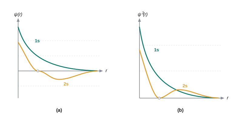
Fig. 2.15 – Wave function and probability density plots for 1s and 2s orbitals.
According to Max Born, the square of the wave function (\(\psi^2\)) at a point gives the probability density of the electron at that point. The variation of \(\psi^2\) against \(r\) for the 1s and 2s orbitals is shown in Fig. 2.15(b), and again the two curves differ.
For the 1s orbital, the probability density is maximum right at the nucleus and decreases sharply as we move away. For the 2s orbital, the probability density first decreases sharply to zero, then rises again to a small maximum, and finally decreases and approaches zero as \(r\) increases further. The region where the probability density falls to zero is called a node (or nodal surface). In general, an ns orbital has \((n-1)\) nodes — so the 2s orbital has one node, the 3s has two, and so on. The number of nodes increases with \(n\).
These probability density variations can be visualised as charge cloud diagrams (Fig. 2.16a), in which the density of the dots in a region represents the electron probability density there.

Fig. 2.16 – Charge cloud and boundary surface diagrams for 1s and 2s orbitals.
A more useful way to show shape is the boundary surface diagram. Here a surface is drawn in space on which the value of the probability density \(|\psi|^2\) is constant. Although many such surfaces are possible, we take the one that encloses a region within which the probability of finding the electron is very high — say about 90%.
One might ask why we don’t draw a boundary surface enclosing 100% of the probability. The reason is that \(|\psi|^2\) always has some small, non-zero value at any finite distance from the nucleus, so no boundary of finite, rigid size could enclose a full 100% probability. The boundary surface for an s orbital is a sphere centred on the nucleus (a circle in two dimensions), enclosing a region of about 90% probability.
So the 1s and 2s orbitals are spherical in shape. In fact all s orbitals are spherically symmetric — the probability of finding the electron at a given distance is the same in every direction. The size of the s orbital increases with \(n\), so that \(4s > 3s > 2s > 1s\), with the electron located further from the nucleus as \(n\) increases.
Boundary surface diagrams for the three 2p orbitals (\(l = 1\)) are shown in Fig. 2.17. Here the nucleus is at the origin, and unlike s orbitals, the p orbitals are not spherical. Each p orbital has two sections called lobes, one on each side of a plane passing through the nucleus. The probability density is zero on this plane where the two lobes meet.
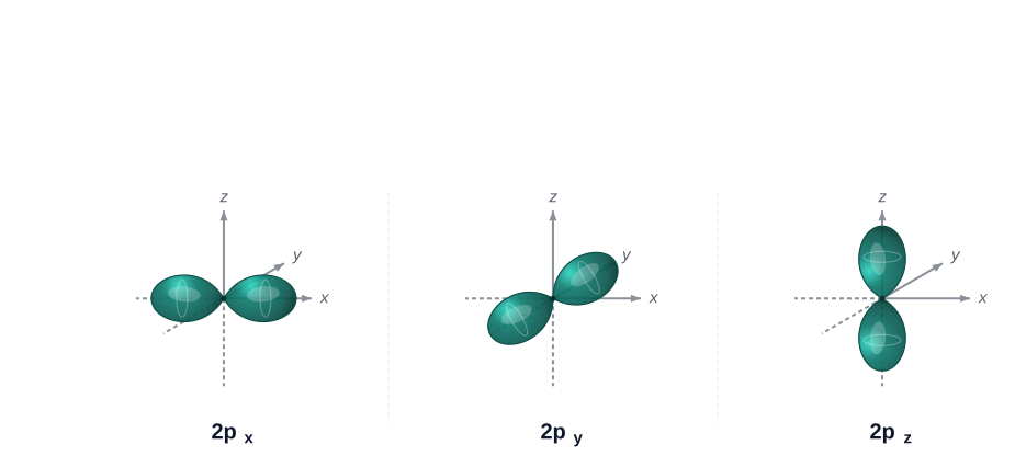
Fig. 2.17 – Boundary surface diagrams of the three 2p orbitals.
The three p orbitals are identical in size, shape, and energy; they differ only in the orientation of their lobes. Since the lobes lie along the x, y, or z axis, the orbitals are labelled \(2p_x\), \(2p_y\), and \(2p_z\). It should be understood, though, that there is no simple one-to-one relation between the values of \(m_l\) (\(-1, 0, +1\)) and the x, y, z directions; for our purpose it is enough to remember that three values of \(m_l\) mean three p orbitals with mutually perpendicular axes.
Like s orbitals, p orbitals grow in size and energy with \(n\), so the order is \(4p > 3p > 2p\). The probability density functions for a p orbital pass through zero (besides at the nucleus and at infinite distance) as the distance from the nucleus increases. The number of such radial nodes is \(n - 2\): one radial node for 3p, two for 4p, and so on.
For \(l = 2\), the orbital is a d-orbital, and the minimum value of \(n\) must be 3 (since \(l\) cannot exceed \(n-1\)). There are five \(m_l\) values (\(-2, -1, 0, +1, +2\)) for \(l = 2\), so there are five d orbitals. Their boundary surface diagrams are shown in Fig. 2.18.
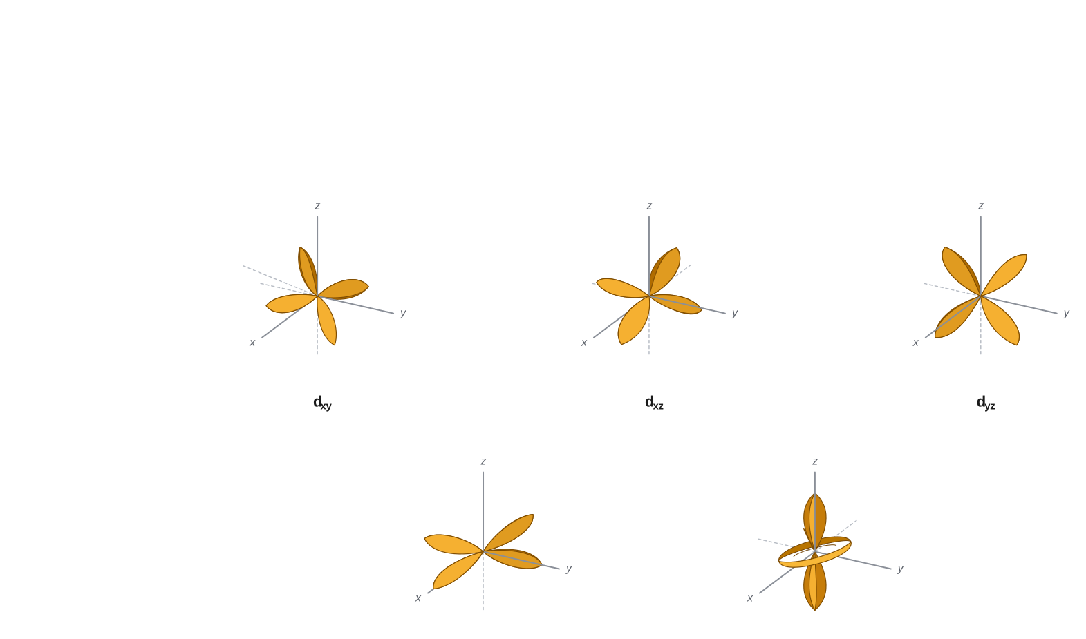
Fig. 2.18 – Boundary surface diagrams of the five 3d orbitals.
The five d orbitals are designated \(d_{xy}\), \(d_{yz}\), \(d_{xz}\), \(d_{x^2-y^2}\), and \(d_{z^2}\). The shapes of the first four are similar to one another, while the shape of the fifth, \(d_{z^2}\), is different — yet all five 3d orbitals are equal in energy. The d orbitals for \(n\) greater than 3 (4d, 5d, …) have shapes similar to 3d but differ in energy and size.
Besides radial nodes (where the probability density is zero), the p and d orbitals also have angular nodes — planes passing through the nucleus (origin) where the probability density is zero. For example, in the \(p_z orbital\) the xy-plane is a nodal plane; in the \(d_{xy}\) orbital there are two nodal planes. The number of angular nodes equals \(l\): one angular node for p orbitals, two for d orbitals, and so on. The total number of nodes is given by \((n-1)\) — that is, \(l\) angular nodes plus \((n - l - 1)\) radial nodes.
2.6.3 Energies of Orbitals
The energy of an electron in a hydrogen atom is determined solely by the principal quantum number \(n\). So the orbital energies in hydrogen increase in the order:
\[1s < 2s = 2p < 3s = 3p = 3d < 4s = 4p = 4d = 4f < \ldots \qquad (2.23)\]
and this is depicted in Fig. 2.19. Notice that although the 2s and 2p orbitals have different shapes, an electron has the same energy in the 2s orbital as in the 2p orbital. Orbitals having the same energy are called degenerate. The 1s orbital in hydrogen corresponds to the most stable condition — the ground state — where the electron is held most tightly by the nucleus. An electron in the 2s, 2p, or higher orbital of hydrogen is in an excited state.
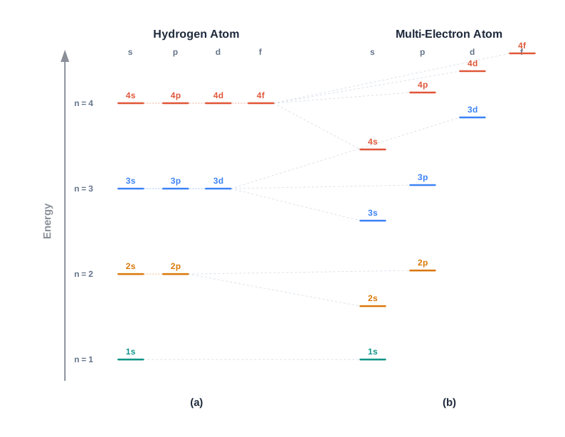
Fig. 2.19 – Energy level diagrams for (a) hydrogen and (b) a multi-electron atom.
The situation is different for a multi-electron atom. Here the energy of an electron depends not only on \(n\) (the shell) but also on \(l\) (the sub-shell). That is, for a given \(n\), the s, p, d, f orbitals all have different energies. Within a given shell, the energy of orbitals increases in the order \(s < p < d < f\). At higher energy levels these differences become large enough that the levels overlap in a staggered way — for example \(4s < 3d\), \(6s < 5d\), and \(4f < 6p\).
Why do the sub-shells have different energies in multi-electron atoms? The main reason is the mutual repulsion among the electrons. In hydrogen, the only electrical interaction is the attraction between the single electron and the nucleus. In a multi-electron atom, besides this attraction, there are repulsions between every electron and all the others. The stability of an electron comes from the total attractive interactions exceeding the total repulsive ones.
Shielding and effective nuclear charge
A key idea here is shielding. In general, the repulsion of an outer-shell electron by the inner-shell electrons is important. The attractive interaction of an electron increases with the positive charge on the nucleus (\(Ze\)). But because inner-shell electrons lie between the nucleus and an outer electron, the outer electron does not feel the full nuclear charge. The inner electrons partly screen (block) the nuclear charge — this is called the shielding of the outer-shell electrons from the nucleus by the inner-shell electrons. The net positive charge actually felt by an outer electron is called the effective nuclear charge, \(Z_{\text{eff}},e\).
Despite this shielding, the attractive force on the outer electrons still increases as the nuclear charge increases. In other words, the energy of interaction between the nucleus and the electron (the orbital energy) becomes more negative as the atomic number \(Z\) increases.
Both the attractive and repulsive interactions depend on the shell and the shape of the orbital the electron is in. For example, an electron in a spherical s orbital shields the outer electrons more effectively than a p-orbital electron; a p-orbital electron shields more than a d-orbital electron, even within the same shell. This happens because, due to the spherical shape of the s orbital, an s electron spends more time close to the nucleus than a p electron, which in turn spends more time near the nucleus than a d electron.
So, for a given shell, the \(Z_{\text{eff}}\) experienced by an electron decreases as \(l\) increases. This means the s electron is more tightly bound than the p electron, which is more tightly bound than the d electron. Correspondingly, the energy of an s electron is lower (more negative) than a p electron, which is lower than a d electron, and so on.
The \((n + l)\) rule
Because the extent of shielding differs for different orbitals, the energy levels within the same shell split, and orbital energy depends on both \(n\) and \(l\). The mathematical dependence is complicated, but one simple rule captures it: the lower the value of \((n + l)\) for an orbital, the lower its energy. If two orbitals have the same \((n + l)\) value, then the orbital with the lower \(n\) has the lower energy.
Table 2.5 illustrates this rule, and Fig. 2.19 depicts the energy levels of multi-electron atoms.
Table 2.5 Arrangement of Orbitals with Increasing Energy on the Basis of \((n+l)\) Rule
| Orbital | Value of \(n\) | Value of \(l\) | Value of \((n+l)\) | |
|---|---|---|---|---|
| 1s | 1 | 0 | \(1 + 0 = 1\) | |
| 2s | 2 | 0 | \(2 + 0 = 2\) | |
| 2p | 2 | 1 | \(2 + 1 = 3\) | 2p (\(n=2\)) has lower energy than 3s (\(n=3\)) |
| 3s | 3 | 0 | \(3 + 0 = 3\) | |
| 3p | 3 | 1 | \(3 + 1 = 4\) | 3p (\(n=3\)) has lower energy than 4s (\(n=4\)) |
| 4s | 4 | 0 | \(4 + 0 = 4\) | 4s (\(n=4\)) |
| 3d | 3 | 2 | \(3 + 2 = 5\) | 3d (\(n=3\)) has lower energy than 4p (\(n=4\)) |
| 4p | 4 | 1 | \(4 + 1 = 5\) | 4p (\(n=4\)) |
Different sub-shells of a shell have different energies in multi-electron atoms, but in hydrogen they have the same energy. Finally, note that the energy of an orbital in the same sub-shell decreases as the atomic number \(Z_{\text{eff}}\) increases. For example, the energy of the 2s orbital of hydrogen is greater than that of lithium, which is greater than that of sodium, and so on: \(E_{2s}(\mathrm{H}) > E_{2s}(\mathrm{Li}) > E_{2s}(\mathrm{Na}) > E_{2s}(\mathrm{K})\).
2.6.4 Filling of Orbitals in Atom
Electrons are filled into the orbitals of atoms according to the aufbau principle, which itself rests on three ideas working together: the Pauli exclusion principle, Hund’s rule of maximum multiplicity, and the relative energies of the orbitals.
Aufbau principle
The German word aufbau means “building up.” Here it refers to building up the electronic structure of an atom by filling its orbitals with electrons.
As we have seen, an orbital’s energy depends on the effective nuclear charge, and different orbitals are affected to different extents. So there is no single ordering of orbital energies that is universally correct for all atoms. However, the following order of orbital energies is extremely useful:
\[1s,\ 2s,\ 2p,\ 3s,\ 3p,\ 4s,\ 3d,\ 4p,\ 5s,\ 4d,\ 5p,\ 6s,\ 4f,\ 5d,\ 6p,\ 7s, \ldots\]
This order can be remembered using the diagonal-arrow method of Fig. 2.20.

Fig. 2.20 – Order of filling of orbitals in a multi-electron atom.
Starting from the top, the direction of the arrows gives the order of filling — from right-top to bottom-left. This scheme is remarkably accurate for the placement of outermost valence electrons. For example, the valence electron in potassium must choose between the 3d and 4s orbitals, and this sequence correctly predicts it goes into 4s. The order should be treated as a rough guide, because in many cases orbitals are close in energy and small changes can alter the filling order — so exceptions do occur.
Flowchart
FC 2.2 – Rules for filling electrons into orbitals (in order): Step 1 Aufbau principle → fill lowest-energy orbital first (use the 1s, 2s, 2p, 3s, 3p, 4s, 3d… order); Step 2 Pauli exclusion principle → each orbital takes at most 2 electrons, and they must have opposite spins; Step 3 Hund’s rule → within a set of degenerate orbitals, place one electron in each (all parallel spins) before any pairing begins → gives the ground-state configuration.
Pauli exclusion principle
The number of electrons an orbital can hold is limited by the exclusion principle, given by Wolfgang Pauli in 1926.
This means two electrons in the same orbital can share the same values of \(n\), \(l\), and \(m_l\), but must differ in the spin quantum number \(m_s\). The restriction lets us calculate the maximum number of electrons a sub-shell can hold. For example, the 1s sub-shell has one orbital, so it holds at most 2 electrons; the p sub-shell holds 6, the d sub-shell holds 10, and so on. Summed up: the maximum number of electrons in the shell with principal quantum number \(n\) is \(2n^2\).
Hund’s rule of maximum multiplicity
This rule deals with how electrons fill orbitals belonging to the same sub-shell — orbitals of equal energy, called degenerate orbitals.
Since there are three p, five d, and seven f orbitals, pairing of electrons begins with the entry of the 4th, 6th, and 8th electron respectively in the p, d, and f sub-shells. It has also been observed that half-filled and fully filled sets of degenerate orbitals have extra stability due to their symmetry (see Section 2.6.6).
2.6.5 Electronic Configuration of Atoms
The distribution of electrons into the orbitals of an atom is called its electronic configuration. Once the filling rules are understood, the electronic configurations of atoms can be written easily. There are two common ways to represent them.
The first is the \(s^a p^b d^c \ldots\) notation. Here the sub-shell is written using its letter symbol, with the number of electrons in it shown as a superscript (a, b, c, …). Sub-shells of different shells are told apart by writing the principal quantum number before the sub-shell symbol.
The second is the orbital diagram, in which each orbital of a sub-shell is drawn as a box, and each electron is shown as an arrow — \(\uparrow\) for positive spin, \(\downarrow\) for negative spin. The advantage of the orbital diagram over the first notation is that it represents all four quantum numbers.

Fig. 2.21 – Representations of electronic configuration and orbital boxes.
Let us build up the configurations of the first several elements. The hydrogen atom has one electron, which goes into the lowest-energy orbital, 1s. Its configuration is \(1s^1\). The second electron in helium (He) also occupies the 1s orbital, giving \(1s^2\); as required by Pauli’s principle, the two electrons have opposite spins.
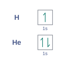
Fig. 2.22 – Orbital box diagrams for hydrogen and helium.
The third electron of lithium (Li) cannot enter the 1s orbital (Pauli’s principle), so it takes the next available orbital, 2s. The configuration of Li is \(1s^2 2s^1\). The 2s orbital can take one more electron, so beryllium (Be) is \(1s^2 2s^2\).
In the next six elements the 2p orbitals fill progressively: boron (B, \(1s^2 2s^2 2p^1\)), carbon (C, \(1s^2 2s^2 2p^2\)), nitrogen (N, \(1s^2 2s^2 2p^3\)), oxygen (O, \(1s^2 2s^2 2p^4\)), fluorine (F, \(1s^2 2s^2 2p^5\)), and neon (Ne, \(1s^2 2s^2 2p^6\)), completing the process at neon.
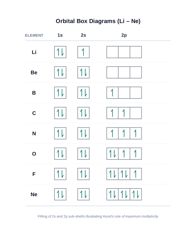
Fig. 2.23 – Orbital box diagrams for elements lithium through neon.
The elements from sodium (Na, \(1s^2 2s^2 2p^6 3s^1\)) to argon (Ar, \(1s^2 2s^2 2p^6 3s^2 3p^6\)) follow exactly the same pattern as lithium to neon, except that now the 3s and 3p orbitals are being filled. We can simplify by writing the electrons of the first two shells as the noble gas neon (Ne): so sodium to argon are written from (Na, [Ne]\(3s^1\)) to (Ar, [Ne]\(3s^2 3p^6\)).
The electrons in completely filled inner shells are called core electrons, and the electrons added to the shell with the highest principal quantum number are called valence electrons. For example, in the elements Na to Ar, the electrons of Ne are the core electrons and the ones beyond are the valence electrons. In potassium (K) and calcium (Ca), the 4s orbital is lower in energy than the 3d, so it is filled by one and two electrons respectively.
A new pattern begins with scandium (Sc). The 3d orbital, being lower in energy than 4p, is filled first. So in the next ten elements — scandium (Sc), titanium (Ti), vanadium (V), chromium (Cr), manganese (Mn), iron (Fe), cobalt (Co), nickel (Ni), copper (Cu), and zinc (Zn) — the five 3d orbitals are progressively occupied.
Two of these, chromium and copper, are surprising: they have five and ten electrons in the 3d orbitals rather than the four and nine that their position suggests (which would leave two electrons in 4s). The reason is that fully filled and half-filled orbitals have extra stability (lower energy). Configurations like \(p^3\), \(p^6\), \(d^5\), \(d^{10}\), \(f^7\), \(f^{14}\) — half-filled or fully filled — are more stable, so chromium and copper adopt the \(d^5\) and \(d^{10}\) configurations (caution: exceptions do exist).
With the 3d orbitals saturated, the 4p orbital fills from gallium (Ga) to krypton (Kr). In the next eighteen elements, from rubidium (Rb) to xenon (Xe), the 5s, 4d, and 5p orbitals fill in a way parallel to the 4s, 3d, and 4p orbitals above. Then comes the 6s orbital: in caesium (Cs) and barium (Ba) it holds one and two electrons. From lanthanum (La) to mercury (Hg), the 4f and 5d orbitals fill. After this, the 6p, then 7s, and finally 5f and 6d orbitals fill. Elements after uranium (U) are all short-lived and are produced artificially. The electronic configurations of the known elements are tabulated in Table 2.6.
Table 2.6 Electronic Configurations of the Elements (elements 1–54)
| Element | Z | 1s | 2s | 2p | 3s | 3p | 3d | 4s | 4p | 4d | 5s | 5p |
|---|---|---|---|---|---|---|---|---|---|---|---|---|
| H | 1 | 1 | ||||||||||
| He | 2 | 2 | ||||||||||
| Li | 3 | 2 | 1 | |||||||||
| Be | 4 | 2 | 2 | |||||||||
| B | 5 | 2 | 2 | 1 | ||||||||
| C | 6 | 2 | 2 | 2 | ||||||||
| N | 7 | 2 | 2 | 3 | ||||||||
| O | 8 | 2 | 2 | 4 | ||||||||
| F | 9 | 2 | 2 | 5 | ||||||||
| Ne | 10 | 2 | 2 | 6 | ||||||||
| Na | 11 | 2 | 2 | 6 | 1 | |||||||
| Mg | 12 | 2 | 2 | 6 | 2 | |||||||
| Al | 13 | 2 | 2 | 6 | 2 | 1 | ||||||
| Si | 14 | 2 | 2 | 6 | 2 | 2 | ||||||
| P | 15 | 2 | 2 | 6 | 2 | 3 | ||||||
| S | 16 | 2 | 2 | 6 | 2 | 4 | ||||||
| Cl | 17 | 2 | 2 | 6 | 2 | 5 | ||||||
| Ar | 18 | 2 | 2 | 6 | 2 | 6 | ||||||
| K | 19 | 2 | 2 | 6 | 2 | 6 | 1 | |||||
| Ca | 20 | 2 | 2 | 6 | 2 | 6 | 2 | |||||
| Sc | 21 | 2 | 2 | 6 | 2 | 6 | 1 | 2 | ||||
| Ti | 22 | 2 | 2 | 6 | 2 | 6 | 2 | 2 | ||||
| V | 23 | 2 | 2 | 6 | 2 | 6 | 3 | 2 | ||||
| Cr* | 24 | 2 | 2 | 6 | 2 | 6 | 5 | 1 | ||||
| Mn | 25 | 2 | 2 | 6 | 2 | 6 | 5 | 2 | ||||
| Fe | 26 | 2 | 2 | 6 | 2 | 6 | 6 | 2 | ||||
| Co | 27 | 2 | 2 | 6 | 2 | 6 | 7 | 2 | ||||
| Ni | 28 | 2 | 2 | 6 | 2 | 6 | 8 | 2 | ||||
| Cu* | 29 | 2 | 2 | 6 | 2 | 6 | 10 | 1 | ||||
| Zn | 30 | 2 | 2 | 6 | 2 | 6 | 10 | 2 | ||||
| Ga | 31 | 2 | 2 | 6 | 2 | 6 | 10 | 2 | 1 | |||
| Ge | 32 | 2 | 2 | 6 | 2 | 6 | 10 | 2 | 2 | |||
| As | 33 | 2 | 2 | 6 | 2 | 6 | 10 | 2 | 3 | |||
| Se | 34 | 2 | 2 | 6 | 2 | 6 | 10 | 2 | 4 | |||
| Br | 35 | 2 | 2 | 6 | 2 | 6 | 10 | 2 | 5 | |||
| Kr | 36 | 2 | 2 | 6 | 2 | 6 | 10 | 2 | 6 | |||
| Rb | 37 | 2 | 2 | 6 | 2 | 6 | 10 | 2 | 6 | 1 | ||
| Sr | 38 | 2 | 2 | 6 | 2 | 6 | 10 | 2 | 6 | 2 | ||
| Y | 39 | 2 | 2 | 6 | 2 | 6 | 10 | 2 | 6 | 1 | 2 | |
| Zr | 40 | 2 | 2 | 6 | 2 | 6 | 10 | 2 | 6 | 2 | 2 | |
| Nb* | 41 | 2 | 2 | 6 | 2 | 6 | 10 | 2 | 6 | 4 | 1 | |
| Mo* | 42 | 2 | 2 | 6 | 2 | 6 | 10 | 2 | 6 | 5 | 1 | |
| Tc | 43 | 2 | 2 | 6 | 2 | 6 | 10 | 2 | 6 | 5 | 2 | |
| Ru* | 44 | 2 | 2 | 6 | 2 | 6 | 10 | 2 | 6 | 7 | 1 | |
| Rh* | 45 | 2 | 2 | 6 | 2 | 6 | 10 | 2 | 6 | 8 | 1 | |
| Pd* | 46 | 2 | 2 | 6 | 2 | 6 | 10 | 2 | 6 | 10 | ||
| Ag* | 47 | 2 | 2 | 6 | 2 | 6 | 10 | 2 | 6 | 10 | 1 | |
| Cd | 48 | 2 | 2 | 6 | 2 | 6 | 10 | 2 | 6 | 10 | 2 | |
| In | 49 | 2 | 2 | 6 | 2 | 6 | 10 | 2 | 6 | 10 | 2 | 1 |
| Sn | 50 | 2 | 2 | 6 | 2 | 6 | 10 | 2 | 6 | 10 | 2 | 2 |
| Sb | 51 | 2 | 2 | 6 | 2 | 6 | 10 | 2 | 6 | 10 | 2 | 3 |
| Te | 52 | 2 | 2 | 6 | 2 | 6 | 10 | 2 | 6 | 10 | 2 | 4 |
| I | 53 | 2 | 2 | 6 | 2 | 6 | 10 | 2 | 6 | 10 | 2 | 5 |
| Xe | 54 | 2 | 2 | 6 | 2 | 6 | 10 | 2 | 6 | 10 | 2 | 6 |
Elements with exceptional electronic configurations. (The configurations of the remaining elements, Cs to element 111, are tabulated in the full NCERT Table 2.6; elements with atomic number 112 and above have been reported but not yet fully authenticated and named.)
Why bother knowing electronic configurations? Because the whole of modern chemistry rests on electron distribution. Questions like why atoms combine to form molecules, why some elements are metals while others are non-metals, why helium and argon are unreactive while the halogens are highly reactive — all find simple explanations in the electronic configuration. None of these questions could be answered by Dalton’s model. A detailed grasp of electronic structure is therefore essential for understanding chemistry.
2.6.6 Stability of Completely Filled and Half Filled Subshells
The ground-state electronic configuration of an atom always corresponds to the state of lowest total electronic energy. Most atoms follow the basic filling rules of Section 2.6.5. But in certain elements, such as copper (Cu) and chromium (Cr), where two sub-shells (4s and 3d) are close in energy, an electron shifts from the lower-energy sub-shell (4s) to the higher-energy one (3d) — provided that this shift makes the higher sub-shell either completely filled or exactly half-filled.
This is exactly what we saw above. The valence configurations of Cr and Cu are therefore \(3d^5 4s^1\) and \(3d^{10} 4s^1\) respectively, and not \(3d^4 4s^2\) and \(3d^9 4s^2\). There is extra stability associated with these half-filled (\(d^5\)) and fully filled (\(d^{10}\)) configurations.
Causes of the extra stability
Two reasons explain why completely filled and half-filled sub-shells are especially stable.
The first is the symmetrical distribution of electrons. Symmetry leads to stability. A completely filled or half-filled sub-shell has a symmetrical distribution of electrons. Electrons in the same sub-shell (say 3d) have equal energy but different spatial distributions, so their shielding of one another is relatively small, and the electrons are held more strongly by the nucleus.
The second reason is exchange energy. Whenever two or more electrons with the same spin are present in the degenerate orbitals of a sub-shell, they can exchange their positions, and the energy released in this process is called exchange energy. The number of possible exchanges is maximum when the sub-shell is exactly half-filled or completely filled, so the exchange energy — and hence the stability — is maximum then.
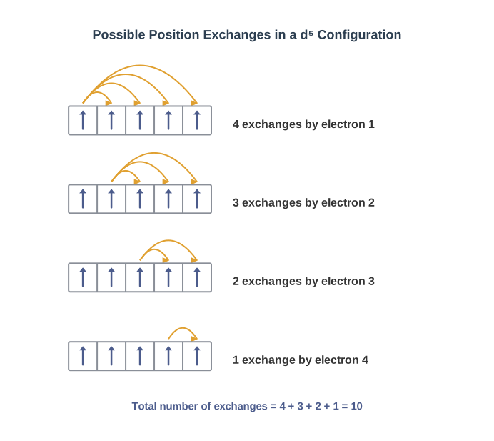
Fig. 2.24 – Possible electron exchanges for a half-filled d⁵ configuration.
The exchange energy is actually the basis of Hund’s rule — it is why electrons entering degenerate orbitals prefer parallel spins as far as possible. To sum up, the extra stability of half-filled and completely filled sub-shells is due to three things: relatively small shielding, smaller coulombic repulsion energy, and larger exchange energy.
2.7 Summary
- Atoms are the building blocks of elements — the smallest parts of an element that take part in chemical reactions. The first atomic theory, given by John Dalton in 1808, treated the atom as the ultimate, indivisible particle of matter.
- Towards the end of the nineteenth century, experiments proved that atoms are divisible and are made of three fundamental particles: electrons, protons, and neutrons. The electron carries a charge of \(-1.602176 \times 10^{-19}\) C, the proton an equal and opposite positive charge, and the neutron no charge; protons and neutrons are almost 1800 times heavier than the electron.
- The atomic number \(Z\) is the number of protons (equal to the number of electrons in a neutral atom); the mass number \(A = Z + n\), where \(n\) is the number of neutrons. Isotopes have the same \(Z\) but different \(A\); isobars have the same \(A\) but different \(Z\).
- The discovery of sub-atomic particles led to various atomic models. Thomson’s model (1898) pictured the atom as a uniform sphere of positive charge with electrons embedded in it, and its mass evenly spread. It explained neutrality but was disproved by Rutherford’s α-particle scattering experiment.
- Rutherford’s model concluded that the atom has a tiny, dense, positively charged nucleus at its centre, with electrons revolving around it in circular orbits. It resembled the solar system and improved on Thomson’s model, but it could not explain the stability of the atom (a moving charged electron should radiate energy and spiral in) and said nothing about the arrangement and energies of the electrons.
- Bohr’s model (1913) overcame these difficulties for the hydrogen atom. Bohr postulated that the electron moves around the nucleus only in certain allowed circular orbits, each of a definite energy, and that energy is absorbed or emitted only when the electron jumps between orbits. He calculated the energies of these orbits and predicted the electron–nucleus distances.
- The energy of the electron in the \(n\)th orbit of hydrogen is \(E_n = -R_H\left(\dfrac{1}{n^2}\right)\), with \(R_H = 2.18 \times 10^{-18}\) J, and the orbit radius is \(r_n = n^2 a_0\) with \(a_0 = 52.9\) pm. The negative energy shows the bound electron is more stable than a free one.
- Bohr’s model explained the line spectrum of hydrogen quantitatively: each spectral line arises from an electron transition, with \(\Delta E = 2.18 \times 10^{-18}\ \text{J}\left(\dfrac{1}{n_i^2} - \dfrac{1}{n_f^2}\right)\). This matches Rydberg’s empirical formula. However, Bohr’s model failed for multi-electron atoms, could not explain the fine structure of spectra or the Zeeman and Stark effects, and could not account for chemical bonding.
- Bohr’s model was rejected because it ignores the wave–particle duality of matter and contradicts the Heisenberg uncertainty principle. De Broglie (\(\lambda = h/mv\)) showed matter has a wave nature, and Heisenberg (\(\Delta x \cdot \Delta p_x \geq h/4\pi\)) showed the position and momentum of an electron cannot both be known exactly, so an electron has no definite orbit.
- Erwin Schrödinger (1926) proposed an equation to describe the electron distributions and allowed energy levels in atoms. It incorporates de Broglie’s duality and is consistent with the uncertainty principle. Solving it for the hydrogen atom gives the possible energy states and the corresponding wave functions \(\psi\).
- These quantised energy states and wave functions are characterised naturally by three quantum numbers: the principal quantum number \(n\), the azimuthal quantum number \(l\), and the magnetic quantum number \(m_l\). The restrictions on their values come out of the solution itself. The quantum mechanical model of the hydrogen atom successfully predicts all aspects of the hydrogen spectrum, including features Bohr’s model could not.
- The electron distribution of an atom is divided into shells, which consist of one or more subshells, which in turn are composed of one or more orbitals. An orbital is the wave function \(\psi\); \(|\psi|^2\) gives the probability density of finding the electron. An orbital holds at most two electrons of opposite spin (a fourth quantum number, \(m_s = \pm\frac{1}{2}\)).
- For hydrogen and hydrogen-like species (He⁺, Li²⁺, etc.), all orbitals of a given shell have the same energy. For multi-electron atoms, orbital energy depends on both \(n\) and \(l\): the lower the value of \((n + l)\), the lower the energy; for equal \((n + l)\), the orbital with lower \(n\) has lower energy.
- Electrons fill orbitals in order of increasing energy in accordance with the Aufbau principle, the Pauli exclusion principle (no two electrons in an atom can have the same set of four quantum numbers), and Hund’s rule of maximum multiplicity (pairing in a subshell does not begin until each orbital of that subshell is singly occupied). This forms the basis of the electronic structure of atoms.
- Completely filled (\(p^6\), \(d^{10}\), \(f^{14}\)) and exactly half-filled (\(p^3\), \(d^5\), \(f^7\)) subshells have extra stability due to symmetrical electron distribution and larger exchange energy; this is why chromium and copper adopt \(3d^5 4s^1\) and \(3d^{10} 4s^1\) configurations.
Flowchart
FC 2.3 – Evolution of the atomic model (overall chapter sequence): Dalton (indivisible atom) → discovery of electron, proton, neutron → Thomson model (positive sphere with embedded electrons) → Rutherford model (nuclear atom, but unstable) → Bohr model (fixed-energy orbits, explains H spectrum but fails for multi-electron atoms) → de Broglie duality + Heisenberg uncertainty → Schrödinger quantum mechanical model (orbitals, quantum numbers, probability picture).
2.8 NCERT Questions
- Calculate the number of electrons which will together weigh one gram.
- Calculate the mass and charge of one mole of electrons.
- Calculate the total number of electrons present in one mole of methane.
- Find (i) the total number and (ii) the total mass of neutrons in 7 mg of \(^{14}\mathrm{C}\). (Assume that mass of a neutron \(= 1.675 \times 10^{-27}\) kg.)
- Find (i) the total number and (ii) the total mass of protons in 34 mg of \(\mathrm{NH_3}\) at STP. Will the answer change if the temperature and pressure are changed?
- How many neutrons and protons are there in the following nuclei? \(^{13}_{\ 6}\mathrm{C}\), \(^{16}_{\ 8}\mathrm{O}\), \(^{24}_{12}\mathrm{Mg}\), \(^{56}_{26}\mathrm{Fe}\), \(^{88}_{38}\mathrm{Sr}\).
- Write the complete symbol for the atom with the given atomic number (Z) and atomic mass (A):
- \(Z = 17\), \(A = 35\);
- \(Z = 92\), \(A = 233\);
- \(Z = 4\), \(A = 9\).
- Yellow light emitted from a sodium lamp has a wavelength (\(\lambda\)) of 580 nm. Calculate the frequency (\(\nu\)) and wavenumber (\(\bar{\nu}\)) of the yellow light.
- Find energy of each of the photons which
- correspond to light of frequency \(3 \times 10^{15}\) Hz;
- have wavelength of 0.50 Å.
- Calculate the wavelength, frequency and wavenumber of a light wave whose period is \(2.0 \times 10^{-10}\) s.
- What is the number of photons of light with a wavelength of 4000 pm that provide 1 J of energy?
- A photon of wavelength \(4 \times 10^{-7}\) m strikes on a metal surface, the work function of the metal being 2.13 eV. Calculate
- the energy of the photon (eV),
- the kinetic energy of the emission, and
- the velocity of the photoelectron (\(1\ \text{eV} = 1.6020 \times 10^{-19}\) J).
- Electromagnetic radiation of wavelength 242 nm is just sufficient to ionise the sodium atom. Calculate the ionisation energy of sodium in kJ mol⁻¹.
- A 25 watt bulb emits monochromatic yellow light of wavelength 0.57 μm. Calculate the rate of emission of quanta per second.
- Electrons are emitted with zero velocity from a metal surface when it is exposed to radiation of wavelength 6800 Å. Calculate threshold frequency (\(\nu_0\)) and work function (\(W_0\)) of the metal.
- What is the wavelength of light emitted when the electron in a hydrogen atom undergoes transition from an energy level with \(n = 4\) to an energy level with \(n = 2\)?
- How much energy is required to ionise a H atom if the electron occupies \(n = 5\) orbit? Compare your answer with the ionization enthalpy of H atom (energy required to remove the electron from \(n = 1\) orbit).
- What is the maximum number of emission lines when the excited electron of a H atom in \(n = 6\) drops to the ground state?
- The energy associated with the first orbit in the hydrogen atom is \(-2.18 \times 10^{-18}\ \text{J atom}^{-1}\). What is the energy associated with the fifth orbit?
- Calculate the radius of Bohr’s fifth orbit for hydrogen atom.
- Calculate the wavenumber for the longest wavelength transition in the Balmer series of atomic hydrogen.
- What is the energy in joules required to shift the electron of the hydrogen atom from the first Bohr orbit to the fifth Bohr orbit, and what is the wavelength of the light emitted when the electron returns to the ground state? The ground state electron energy is \(-2.18 \times 10^{-11}\) ergs.
- The electron energy in hydrogen atom is given by \(E_n = (-2.18 \times 10^{-18})/n^2\) J. Calculate the energy required to remove an electron completely from the \(n = 2\) orbit. What is the longest wavelength of light in cm that can be used to cause this transition?
- Calculate the wavelength of an electron moving with a velocity of \(2.05 \times 10^7\ \text{m s}^{-1}\).
- The mass of an electron is \(9.1 \times 10^{-31}\) kg. If its K.E. is \(3.0 \times 10^{-25}\) J, calculate its wavelength.
- Which of the following are isoelectronic species, i.e., those having the same number of electrons? \(\mathrm{Na^+}\), \(\mathrm{K^+}\), \(\mathrm{Mg^{2+}}\), \(\mathrm{Ca^{2+}}\), \(\mathrm{S^{2-}}\), Ar.
- Write the electronic configurations of the following ions: (i) H⁻ (ii) Na⁺ (iii) O²⁻ (iv) F⁻.
- What are the atomic numbers of elements whose outermost electrons are represented by (i) \(3s^1\) (ii) \(2p^3\) and (iii) \(3p^5\)?
- Which atoms are indicated by the following configurations? (i) [He]\(2s^1\) (ii) [Ne]\(3s^2 3p^3\) (iii) [Ar]\(4s^2 3d^1\).
- What is the lowest value of \(n\) that allows g orbitals to exist?
- An electron is in one of the 3d orbitals. Give the possible values of \(n\), \(l\) and \(m_l\) for this electron.
- An atom of an element contains 29 electrons and 35 neutrons. Deduce
- the number of protons and
- the electronic configuration of the element.
- Give the number of electrons in the species \(\mathrm{H_2^+}\), \(\mathrm{H_2}\) and \(\mathrm{O_2^+}\).
- An atomic orbital has \(n = 3\). What are the possible values of \(l\) and \(m_l\)?
- List the quantum numbers (\(m_l\) and \(l\)) of electrons for 3d orbital.
- Which of the following orbitals are possible? 1p, 2s, 2p and 3f.
- Using s, p, d notations, describe the orbital with the following quantum numbers:
- \(n = 1\), \(l = 0\);
- \(n = 3\), \(l = 1\);
- \(n = 4\), \(l = 2\);
- \(n = 4\), \(l = 3\).
- Explain, giving reasons, which of the following sets of quantum numbers are not possible.
- \(n = 0\), \(l = 0\), \(m_l = 0\), \(m_s = +\frac{1}{2}\);
- \(n = 1\), \(l = 0\), \(m_l = 0\), \(m_s = -\frac{1}{2}\);
- \(n = 1\), \(l = 1\), \(m_l = 0\), \(m_s = +\frac{1}{2}\);
- \(n = 2\), \(l = 1\), \(m_l = 0\), \(m_s = -\frac{1}{2}\);
- \(n = 3\), \(l = 3\), \(m_l = -3\), \(m_s = +\frac{1}{2}\);
- \(n = 3\), \(l = 1\), \(m_l = 0\), \(m_s = +\frac{1}{2}\).
- How many electrons in an atom may have the following quantum numbers?
- \(n = 4\), \(m_s = -\frac{1}{2}\);
- \(n = 3\), \(l = 0\).
- Show that the circumference of the Bohr orbit for the hydrogen atom is an integral multiple of the de Broglie wavelength associated with the electron revolving around the orbit.
- What transition in the hydrogen spectrum would have the same wavelength as the Balmer transition \(n = 4\) to \(n = 2\) of He⁺ spectrum?
- Calculate the energy required for the process \(\mathrm{He^+}\text{(g)} \rightarrow \mathrm{He^{2+}}\text{(g)} + \mathrm{e^-}\). The ionization energy for the H atom in the ground state is \(2.18 \times 10^{-18}\ \text{J atom}^{-1}\).
- If the diameter of a carbon atom is 0.15 nm, calculate the number of carbon atoms which can be placed side by side in a straight line across a length of a scale 20 cm long.
- \(2 \times 10^8\) atoms of carbon are arranged side by side. Calculate the radius of a carbon atom if the length of this arrangement is 2.4 cm.
- The diameter of a zinc atom is 2.6 Å. Calculate
- the radius of the zinc atom in pm and
- the number of atoms present in a length of 1.6 cm if the zinc atoms are arranged side by side lengthwise.
- A certain particle carries \(2.5 \times 10^{-16}\) C of static electric charge. Calculate the number of electrons present in it.
- In Millikan’s experiment, static electric charge on the oil drops has been obtained by shining X-rays. If the static electric charge on the oil drop is \(-1.282 \times 10^{-18}\) C, calculate the number of electrons present on it.
- In Rutherford’s experiment, generally the thin foil of heavy atoms, like gold, platinum etc., has been used to be bombarded by the α-particles. If the thin foil of light atoms like aluminium etc. is used, what difference would be observed from the above results?
- Symbols \(^{79}_{35}\mathrm{Br}\) and \(^{79}\mathrm{Br}\) can be written, whereas symbols \(^{35}_{79}\mathrm{Br}\) and \(^{35}\mathrm{Br}\) are not acceptable. Answer briefly.
- An element with mass number 81 contains 31.7% more neutrons as compared to protons. Assign the atomic symbol.
- An ion with mass number 37 possesses one unit of negative charge. If the ion contains 11.1% more neutrons than the electrons, find the symbol of the ion.
- An ion with mass number 56 contains 3 units of positive charge and 30.4% more neutrons than electrons. Assign the symbol to this ion.
- Arrange the following type of radiations in increasing order of frequency:
- radiation from microwave oven
- amber light from traffic signal
- radiation from FM radio
- cosmic rays from outer space and
- X-rays.
- Nitrogen laser produces a radiation at a wavelength of 337.1 nm. If the number of photons emitted is \(5.6 \times 10^{24}\), calculate the power of this laser.
- Neon gas is generally used in the sign boards. If it emits strongly at 616 nm, calculate
- the frequency of emission,
- distance traveled by this radiation in 30 s,
- energy of quantum and
- number of quanta present if it produces 2 J of energy.
- In astronomical observations, signals observed from the distant stars are generally weak. If the photon detector receives a total of \(3.15 \times 10^{-18}\) J from the radiations of 600 nm, calculate the number of photons received by the detector.
- Lifetimes of the molecules in the excited states are often measured by using pulsed radiation source of duration nearly in the nanosecond range. If the radiation source has the duration of 2 ns and the number of photons emitted during the pulse source is \(2.5 \times 10^{15}\), calculate the energy of the source.
- The longest wavelength doublet absorption transition is observed at 589 and 589.6 nm. Calculate the frequency of each transition and energy difference between two excited states.
- The work function for caesium atom is 1.9 eV. Calculate
- the threshold wavelength and
- the threshold frequency of the radiation. If the caesium element is irradiated with a wavelength 500 nm, calculate the kinetic energy and the velocity of the ejected photoelectron.
- Following results are observed when sodium metal is irradiated with different wavelengths. Calculate
- threshold wavelength and
- Planck’s constant. \(\lambda\) (nm): 500, 450, 400; \(v \times 10^{-5}\ (\text{cm s}^{-1})\): 2.55, 4.35, 5.35.
- The ejection of the photoelectron from the silver metal in the photoelectric effect experiment can be stopped by applying the voltage of 0.35 V when the radiation 256.7 nm is used. Calculate the work function for silver metal.
- If the photon of wavelength 150 pm strikes an atom and one of its inner bound electrons is ejected out with a velocity of \(1.5 \times 10^7\ \text{m s}^{-1}\), calculate the energy with which it is bound to the nucleus.
- Emission transitions in the Paschen series end at orbit \(n = 3\) and start from orbit \(n\) and can be represented as \(\nu = 3.29 \times 10^{15}\ (\text{Hz}),[1/3^2 - 1/n^2]\). Calculate the value of \(n\) if the transition is observed at 1285 nm. Find the region of the spectrum.
- Calculate the wavelength for the emission transition if it starts from the orbit having radius 1.3225 nm and ends at 211.6 pm. Name the series to which this transition belongs and the region of the spectrum.
- Dual behaviour of matter proposed by de Broglie led to the discovery of electron microscope, often used for the highly magnified images of biological molecules and other types of material. If the velocity of the electron in this microscope is \(1.6 \times 10^6\ \text{m s}^{-1}\), calculate the de Broglie wavelength associated with this electron.
- Similar to electron diffraction, neutron diffraction microscope is also used for the determination of the structure of molecules. If the wavelength used here is 800 pm, calculate the characteristic velocity associated with the neutron.
- If the velocity of the electron in Bohr’s first orbit is \(2.19 \times 10^6\ \text{m s}^{-1}\), calculate the de Broglie wavelength associated with it.
- The velocity associated with a proton moving in a potential difference of 1000 V is \(4.37 \times 10^5\ \text{m s}^{-1}\). If the hockey ball of mass 0.1 kg is moving with this velocity, calculate the wavelength associated with this velocity.
- If the position of the electron is measured within an accuracy of \(\pm 0.002\) nm, calculate the uncertainty in the momentum of the electron. Suppose the momentum of the electron is \(h/4\pi_m \times 0.05\) nm, is there any problem in defining this value?
- The quantum numbers of six electrons are given below. Arrange them in order of increasing energies. If any of these combination(s) has/have the same energy, list them:
- \(n = 4\), \(l = 2\), \(m_l = -2\), \(m_s = -1/2\)
- \(n = 3\), \(l = 2\), \(m_l = 1\), \(m_s = +1/2\)
- \(n = 4\), \(l = 1\), \(m_l = 0\), \(m_s = +1/2\)
- \(n = 3\), \(l = 2\), \(m_l = -2\), \(m_s = -1/2\)
- \(n = 3\), \(l = 1\), \(m_l = -1\), \(m_s = +1/2\)
- \(n = 4\), \(l = 1\), \(m_l = 0\), \(m_s = +1/2\)
- The bromine atom possesses 35 electrons. It contains 6 electrons in 2p orbital, 6 electrons in 3p orbital and 5 electrons in 4p orbital. Which of these electrons experiences the lowest effective nuclear charge?
- Among the following pairs of orbitals which orbital will experience the larger effective nuclear charge?
- 2s and 3s,
- 4d and 4f,
- 3d and 3p.
- The unpaired electrons in Al and Si are present in 3p orbital. Which electrons will experience more effective nuclear charge from the nucleus?
- Indicate the number of unpaired electrons in:
- P,
- Si,
- Cr,
- Fe and
- Kr.
- How many subshells are associated with \(n = 4\)?
- How many electrons will be present in the subshells having \(m_s\) value of \(-1/2\) for \(n = 4\)?