Chapter 4: Chemical Bonding and Molecular Structure
In 1916, a chemist named Gilbert Newton Lewis stood before a puzzle that had troubled scientists for decades: why do atoms join together at all, and why only in certain combinations? Working in his laboratory in the United States, Lewis began sketching atoms not as featureless balls but as tiny cubes, with electrons sitting at the corners. A sodium atom, he reasoned, carried a single electron on one corner, while a noble gas like neon had all eight corners filled. That filled set of eight — an “octet” — seemed to be nature’s mark of stability.
From this simple picture came a powerful idea. Atoms could reach the same comfortable eight-electron arrangement in two ways: by giving away or grabbing electrons, or by sharing them. Sodium hands its lone electron to chlorine; two chlorine atoms instead share a pair between them. In that one insight lay the seed of both the ionic bond and the covalent bond. A few years later, another scientist, Irving Langmuir, polished Lewis’s ideas and gave us the word “covalent.”
Lewis had no computers and no way to see an atom. He had only careful reasoning and a box-shaped sketch. Yet his notation — dots around a chemical symbol — is still taught in every chemistry classroom today, more than a century later.
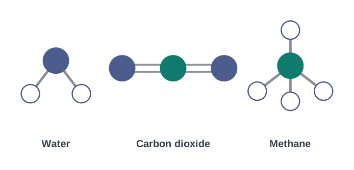
Fig. 4.0 – Ball-and-stick models of water, carbon dioxide and methane.
By the end of this chapter, you will be able to reason your way to the answers to all of these questions.
4.1 Kössel–Lewis Approach to Chemical Bonding
For a long time chemists could see that atoms combine, but they could not say why. The first satisfying answer came in 1916, when two scientists working separately — Walther Kössel and Gilbert N. Lewis — arrived at the same central idea. Both of them built their explanation of valence (the combining capacity of an atom) on one striking clue: the almost complete unreactivity of the noble gases.
The noble gases — helium, neon, argon and the rest — sit quietly in nature and rarely combine with anything. If these elements are so stable, Kössel and Lewis reasoned, then their electron arrangement must be especially stable too. Every other atom, they suggested, tries to reach that same stable arrangement, and that striving is what drives chemical bonding.
The stable octet and Lewis symbols
Lewis pictured an atom as a positively charged kernel — the nucleus together with all the inner-shell electrons — surrounded by an outer shell that could hold a maximum of eight electrons. He imagined these eight outer electrons sitting at the eight corners of a cube around the kernel.
In this picture, sodium’s single outer electron occupies just one corner of the cube, while a noble gas has all eight corners filled. This complete set of eight electrons — the octet — is a particularly stable electronic arrangement. Lewis postulated that atoms achieve this stable octet when they are joined by chemical bonds.
There are two ways to reach the octet. Sodium and chlorine do it by transferring an electron: the electron passes from sodium to chlorine, producing a positive sodium ion (\(\mathrm{Na^+}\)) and a negative chloride ion (\(\mathrm{Cl^-}\)). A cation is a positively charged ion (it has lost electrons); an anion is a negatively charged ion (it has gained electrons). In molecules such as \(\mathrm{Cl_2}\), \(\mathrm{H_2}\) and \(\mathrm{F_2}\), the atoms instead share a pair of electrons, and in doing so each atom attains a stable outer octet.
Only the outermost electrons take part in this combination. These are the valence electrons. The inner-shell electrons lie deep inside the atom, well shielded, and generally play no part in bonding.
To keep track of valence electrons, Lewis introduced a simple notation now called the Lewis symbol: the chemical symbol of the element, with one dot for each valence electron placed around it. The Lewis symbols of the second-period elements are shown in Fig. 4.1.

Fig. 4.1 – Lewis symbols of the second-period elements.
The number of dots around the symbol tells us the number of valence electrons, and from this we can work out the group valence of the element. The group valence is generally either equal to the number of dots (valence electrons) or equal to 8 minus that number — whichever is smaller, since an atom prefers the shorter route to an octet.
Kössel’s key observations
Kössel drew attention to a set of connected facts about the periodic table and ion formation:
- In the periodic table, the highly electronegative halogens (which pull electrons strongly) and the highly electropositive alkali metals (which lose electrons easily) are separated by the noble gases.
- The formation of a negative ion from a halogen atom and a positive ion from an alkali metal is linked to the gain and the loss of an electron by the respective atoms.
- The ions so formed attain stable noble-gas electron configurations. Every noble gas (except helium, which has only a stable duplet of two electrons) has the stable outer octet \(ns^2np^6\).
- The positive and negative ions are then held together by electrostatic attraction — the natural pull between opposite charges.
Following this scheme, the formation of sodium chloride from sodium and chlorine can be shown as an electron transfer. Sodium loses one electron:
\[\mathrm{Na}\ ([\mathrm{Ne}],3s^1) \longrightarrow \mathrm{Na^+}\ ([\mathrm{Ne}]) + \mathrm{e^-}\]
Chlorine gains that electron:
\[\mathrm{Cl}\ ([\mathrm{Ne}],3s^2,3p^5) + \mathrm{e^-} \longrightarrow \mathrm{Cl^-}\ ([\mathrm{Ne}],3s^2,3p^6 \text{ or } [\mathrm{Ar}])\]
The oppositely charged ions then attract each other:
\[\mathrm{Na^+} + \mathrm{Cl^-} \longrightarrow \mathrm{NaCl}\ \text{ or }\ \mathrm{Na^+Cl^-}\]
The formation of calcium fluoride, \(\mathrm{CaF_2}\), follows the same idea, except that calcium must lose two electrons and therefore needs two fluorine atoms to accept them:
\[\mathrm{Ca}\ ([\mathrm{Ar}],4s^2) \longrightarrow \mathrm{Ca^{2+}}\ ([\mathrm{Ar}]) + 2\mathrm{e^-}\]
\[\mathrm{F}\ ([\mathrm{He}],2s^2,2p^5) + \mathrm{e^-} \longrightarrow \mathrm{F^-}\ ([\mathrm{He}],2s^2,2p^6 \text{ or } [\mathrm{Ne}])\]
\[\mathrm{Ca^{2+}} + 2\mathrm{F^-} \longrightarrow \mathrm{CaF_2}\ \text{ or }\ \mathrm{Ca^{2+}(F^-)_2}\]
The bond formed by the electrostatic attraction between the positive and negative ions is called the electrovalent bond. The electrovalence of an atom is simply the number of unit charges on the ion it forms. Thus calcium is assigned a positive electrovalence of two, and chlorine a negative electrovalence of one.
Kössel’s ideas became the foundation of the modern understanding of ion formation, electron transfer and the building of ionic crystalline compounds. At the same time, Kössel himself recognised that a great many compounds simply did not fit this transfer-only picture — a gap that the idea of shared electrons would fill.
4.1.1 Octet Rule
Building on their 1916 work, Kössel and Lewis developed an important idea called the electronic theory of chemical bonding. According to this theory, atoms combine either by the transfer of valence electrons from one atom to another (gaining or losing electrons), or by the sharing of valence electrons, so as to complete an octet in their valence shells. This general statement is known as the octet rule.
Notice the two routes tucked inside this one rule: transfer gives ionic bonding, while sharing gives covalent bonding. The whole of this chapter unfolds from that single split.
4.1.2 Covalent Bond
In 1919 Irving Langmuir refined the Lewis picture. He dropped the idea of electrons sitting fixed at the corners of a cube and introduced the term covalent bond for a bond formed by sharing electrons.
The sharing idea is easiest to see in the chlorine molecule, \(\mathrm{Cl_2}\). A chlorine atom has the configuration \([\mathrm{Ne}],3s^2,3p^5\), which is one electron short of argon. Two chlorine atoms each contribute one electron to a shared pair; that shared pair now “belongs” to both atoms, and each chlorine achieves the outer octet of argon. The shared pair is drawn as a pair of dots (or a line) between the two atoms, as shown in Fig. 4.2.
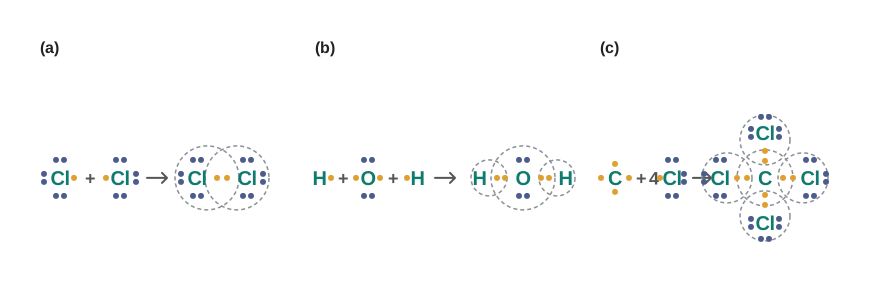
Fig. 4.2 – Formation of covalent bonds by electron sharing.
These dot pictures are called Lewis dot structures. They can be written for many molecules, whether the combining atoms are the same or different, provided a few conditions are met:
- Each bond is formed by the sharing of an electron pair between the atoms.
- Each combining atom contributes at least one electron to the shared pair.
- Through this sharing, the combining atoms attain outer-shell noble-gas configurations.
Water (\(\mathrm{H_2O}\)) and carbon tetrachloride (\(\mathrm{CCl_4}\)) are also drawn in Fig. 4.2, showing how each hydrogen reaches a duplet and each of oxygen, carbon and chlorine reaches an octet.
Single, double and triple bonds
When two atoms share just one electron pair, they are joined by a single covalent bond. In many compounds, however, atoms share more than one pair, giving multiple bonds.
If two atoms share two pairs of electrons, the bond between them is a double bond. In carbon dioxide there are two double bonds, one between carbon and each oxygen; in ethene (\(\mathrm{C_2H_4}\)) the two carbon atoms are joined by a double bond. These are shown in Fig. 4.3.
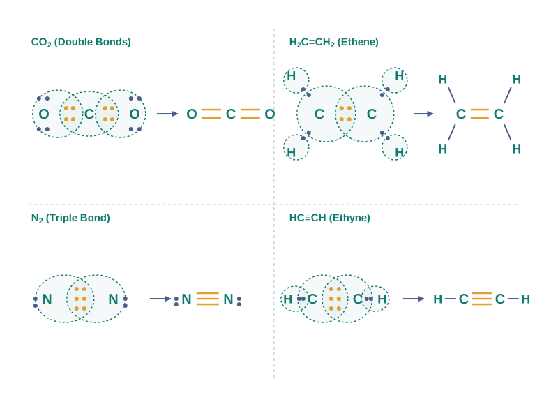
Fig. 4.3 – Lewis structures for molecules with double and triple bonds.
If two atoms share three pairs of electrons, they are joined by a triple bond. This happens between the two nitrogen atoms in the \(\mathrm{N_2}\) molecule and between the two carbon atoms in the ethyne (acetylene, \(\mathrm{C_2H_2}\)) molecule, also drawn in Fig. 4.3.
4.1.3 Lewis Representation of Simple Molecules (the Lewis Structures)
Lewis dot structures give a useful picture of bonding in molecules and ions, in terms of shared pairs of electrons and the octet rule. Such a picture cannot explain everything about how a molecule behaves, but it helps a great deal in understanding how a molecule forms and what its properties are likely to be. A Lewis dot structure can be written by following these steps:
- Find the total number of electrons needed for the structure by adding the valence electrons of all the combining atoms. For example, in the \(\mathrm{CH_4}\) molecule there are eight valence electrons available (4 from carbon and 4 from the four hydrogen atoms).
- For an anion, add one electron for each unit of negative charge; for a cation, subtract one electron for each unit of positive charge. For instance, the \(\mathrm{CO_3^{2-}}\) ion has two extra electrons beyond those supplied by the neutral atoms, while the \(\mathrm{NH_4^+}\) ion has one electron fewer.
- Knowing the chemical symbols and the skeletal (framework) arrangement of the atoms — known or intelligently guessed — distribute the total electrons as bonding shared pairs between the atoms, in proportion to the number of bonds.
- In general, the least electronegative atom occupies the central position. For example, in \(\mathrm{NF_3}\) and \(\mathrm{CO_3^{2-}}\), nitrogen and carbon are the central atoms, while the more electronegative fluorine and oxygen atoms sit at the terminal positions.
- After using up shared pairs for the single bonds, the leftover electron pairs are either used to form multiple bonds or kept as lone pairs (pairs of electrons not involved in bonding). The guiding requirement is that each bonded atom finishes with an octet.
Lewis representations of a few molecules and ions are collected in Table 4.1; the actual dot pictures are drawn in Fig. 4.4.
Table 4.1 The Lewis Representation of Some Molecules
| Molecule/Ion | Lewis representation (described) |
|---|---|
| \(\mathrm{H_2}\) | H : H, i.e. H–H (each H attains a duplet, the configuration of helium) |
| \(\mathrm{O_2}\) | :Ö::Ö:, i.e. O=O with two lone pairs on each O |
| \(\mathrm{O_3}\) | bent O–O–O with one O–O single and one O=O double bond, plus lone pairs |
| \(\mathrm{NF_3}\) | N central, single-bonded to three F atoms; lone pair on N, three lone pairs on each F |
| \(\mathrm{CO_3^{2-}}\) | C central, bonded to three O; one C=O and two C–O⁻; overall charge \(2-\) |
| \(\mathrm{HNO_3}\) | H–O–N with one N=O and one N–O; formal \(+\) on N and \(-\) on an O |
Each H atom attains the configuration of helium (a duplet of electrons).
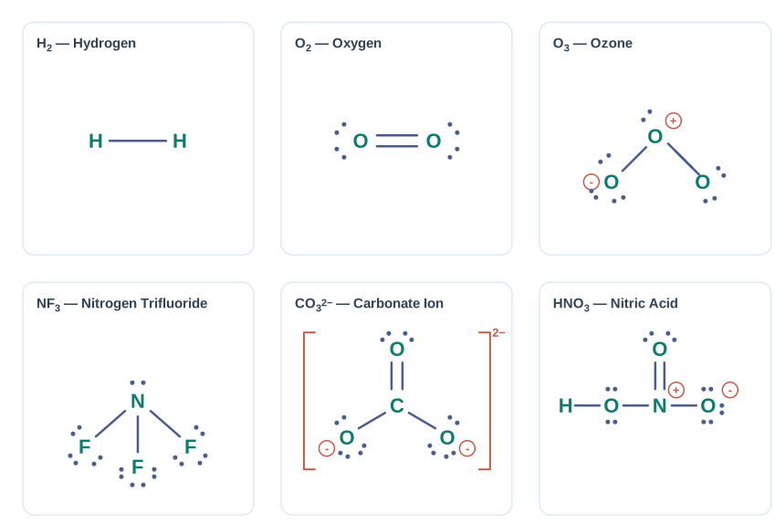
Fig. 4.4 – Lewis dot structures of selected molecules and ions.
Write the Lewis dot structure of the CO molecule.
Step 1. Count the total number of valence electrons of carbon and oxygen. Their outer-shell configurations are \(2s^2,2p^2\) and \(2s^2,2p^4\), so the valence electrons available are \(4 + 6 = 10\).
Step 2. Write the skeletal structure of CO as: C O.
Step 3. Draw a single bond (one shared pair) between C and O, and complete the octet on O. The remaining two electrons form a lone pair on C.
This does not complete the octet on carbon. We therefore resort to multiple bonding — in this case a triple bond between C and O. This satisfies the octet rule for both atoms:
\[\mathrm{:C!\equiv!O:}\]
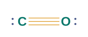
[Caption:] Fig. 4.5 – Lewis structure of the carbon monoxide molecule. [/Caption:]
Write the Lewis structure of the nitrite ion, \(\mathrm{NO_2^-}\).
Step 1. Count the total number of valence electrons of the nitrogen atom, the two oxygen atoms and the one extra electron from the negative charge. With \(\mathrm{N},(2s^2,2p^3)\) and \(\mathrm{O},(2s^2,2p^4)\):
\[5 + (2 \times 6) + 1 = 18\ \text{electrons}\]
Step 2. Write the skeletal structure of \(\mathrm{NO_2^-}\) as: O N O.
Step 3. Draw a single bond between nitrogen and each oxygen, completing the octets on the oxygen atoms. If the remaining two electrons are placed as a lone pair on nitrogen, however, nitrogen’s octet is not complete.
We must therefore use multiple bonding between nitrogen and one of the oxygen atoms (a double bond here). This leads to two equivalent Lewis dot structures, which represent the ion as a resonance pair.
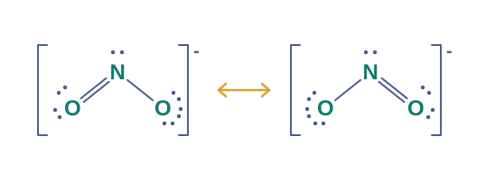
[Caption:] Fig. 4.6 – Resonance structures of the nitrite ion. [/Caption:]
4.1.4 Formal Charge
Lewis dot structures do not, in general, show the true shape of a molecule. Also, in a polyatomic ion the net charge belongs to the ion as a whole, not to any single atom. Even so, it is useful to assign a bookkeeping charge — the formal charge — to each atom.
The formal charge of an atom in a polyatomic molecule or ion is the difference between the number of valence electrons of that atom in its free (isolated) state and the number of electrons “assigned” to it in the Lewis structure.
Written as a compact expression:
\[\text{Formal charge} = N_{\text{v}} - N_{\text{n}} - \tfrac{1}{2},N_{\text{b}}\]
where \(N_{\text{v}}\) is the number of valence electrons in the free atom, \(N_{\text{n}}\) is the number of non-bonding (lone-pair) electrons on that atom, and \(N_{\text{b}}\) is the number of bonding (shared) electrons around it. The counting rests on a simple assumption: an atom “owns” one electron of every shared pair it is part of, and both electrons of each of its lone pairs.
Consider the ozone molecule, \(\mathrm{O_3}\), whose Lewis structure has the three oxygen atoms numbered 1 (central), 2 and 3, as drawn in Fig. 4.7.
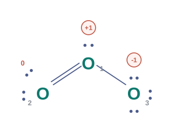
Fig. 4.7 – Lewis structure of ozone with formal charges.
The formal charge on the central O atom (atom 1) is:
\[6 - 2 - \tfrac{1}{2}(6) = +1\]
The formal charge on the end O atom (atom 2) is:
\[6 - 4 - \tfrac{1}{2}(4) = 0\]
The formal charge on the end O atom (atom 3) is:
\[6 - 6 - \tfrac{1}{2}(2) = -1\]
So ozone is represented with a \(+1\) on the central oxygen and a \(-1\) on one end oxygen; the charges add up to zero, as they must for a neutral molecule.
We must be clear that formal charges do not indicate real charge separation within the molecule. Marking them simply helps us keep track of the valence electrons. Their real usefulness is in choosing, from several possible Lewis structures, the one likely to be the most stable.
Generally, the lowest-energy structure is the one with the smallest formal charges on the atoms. Formal charge is based on a purely covalent view of bonding, in which electron pairs are imagined to be shared equally by neighbouring atoms.
4.1.5 Limitations of the Octet Rule
The octet rule is useful, but it is not a universal law. It works best for the structures of most organic compounds and applies mainly to the second-period elements of the periodic table. There are three well-known types of exceptions, together with some further shortcomings.
The incomplete octet of the central atom
In some compounds the central atom is surrounded by fewer than eight electrons. This happens especially with elements that have fewer than four valence electrons. Examples are lithium chloride (\(\mathrm{LiCl}\)), beryllium hydride (\(\mathrm{BeH_2}\)) and boron trichloride (\(\mathrm{BCl_3}\)), shown in Fig. 4.8(a). Lithium, beryllium and boron have only 1, 2 and 3 valence electrons respectively, so their central atoms cannot reach eight. Aluminium chloride (\(\mathrm{AlCl_3}\)) and boron trifluoride (\(\mathrm{BF_3}\)) behave the same way.
Odd-electron molecules
In molecules with an odd total number of electrons — such as nitric oxide (\(\mathrm{NO}\)) and nitrogen dioxide (\(\mathrm{NO_2}\)) — the octet rule cannot be satisfied for all the atoms at once, because an odd number of electrons cannot be split into pairs everywhere. These are drawn in Fig. 4.8(b).
The expanded octet
Elements in and beyond the third period of the periodic table have empty \(3d\) orbitals available for bonding, in addition to their \(3s\) and \(3p\) orbitals. In a number of their compounds, the central atom ends up with more than eight valence electrons around it. This is called the expanded octet, and clearly the octet rule does not apply to such cases.
Examples of compounds with an expanded octet include phosphorus pentafluoride (\(\mathrm{PF_5}\)), sulphur hexafluoride (\(\mathrm{SF_6}\)), sulphuric acid (\(\mathrm{H_2SO_4}\)) and many coordination compounds, shown in Fig. 4.8(c). Interestingly, sulphur also forms many compounds that do obey the octet rule; in sulphur dichloride (\(\mathrm{SCl_2}\)), the sulphur atom has a complete octet around it.
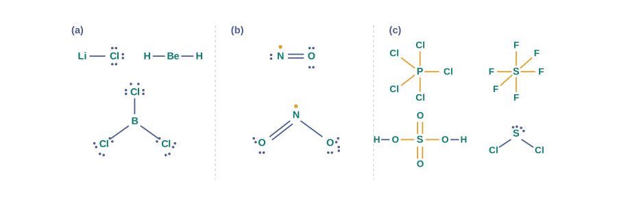
Fig. 4.8 – Exceptions to the octet rule.
Other drawbacks of the octet theory
Beyond these three exceptions, the octet theory has some deeper weaknesses:
- The rule is based on the chemical inertness of the noble gases. Yet some noble gases — for example xenon and krypton — do combine with oxygen and fluorine to form compounds such as \(\mathrm{XeF_2}\), \(\mathrm{KrF_2}\) and \(\mathrm{XeOF_2}\). The “noble gases never react” assumption is therefore not strictly true.
- The theory says nothing about the shape of a molecule.
- It is completely silent about the energy of a molecule, so it cannot explain the relative stability of different molecules.
These gaps are exactly what the later theories in this chapter — VSEPR theory, valence bond theory and molecular orbital theory — are built to fill.
4.2 Ionic or Electrovalent Bond
We have already seen that an electrovalent (ionic) bond arises from the electrostatic attraction between oppositely charged ions. Following the Kössel–Lewis treatment, the formation of an ionic compound depends mainly on two things:
- the ease with which the positive and negative ions can be formed from the respective neutral atoms; and
- the arrangement of these positive and negative ions in the solid — that is, the lattice of the crystalline compound.
Forming the ions: ionization and electron gain
Making a positive ion means ionization — pulling one or more electrons away from a neutral atom. Making a negative ion means adding one or more electrons to a neutral atom. Bringing the two together, we can picture the formation of an ionic solid MX in three steps:
\[\mathrm{M}\text{(g)} \longrightarrow \mathrm{M^+}\text{(g)} + \mathrm{e^-} \qquad (\text{ionization enthalpy})\]
\[\mathrm{X}\text{(g)} + \mathrm{e^-} \longrightarrow \mathrm{X^-}\text{(g)} \qquad (\text{electron gain enthalpy})\]
\[\mathrm{M^+}\text{(g)} + \mathrm{X^-}\text{(g)} \longrightarrow \mathrm{MX}\text{(s)}\]
The electron gain enthalpy, \(\Delta_{eg}H\), is the enthalpy change (introduced in Chapter 3) when a gas-phase atom in its ground state gains an electron. This process can be either exothermic (energy released) or endothermic (energy absorbed), depending on the atom. Ionization, on the other hand, is always endothermic — energy must always be supplied to tear an electron away from an atom. Closely related to electron gain enthalpy is the electron affinity, which is the negative of the energy change accompanying electron gain.
From these two quantities we can see when an ionic bond will form easily.
Most ionic compounds therefore have their cations from metallic elements and their anions from non-metallic elements. The ammonium ion, \(\mathrm{NH_4^+}\) — which is built from two non-metallic elements, nitrogen and hydrogen — is an exception; it acts as the cation in a number of ionic compounds.
The ionic crystal
Ionic compounds in the solid state are not made of separate MX “molecules.” Instead, they consist of orderly, three-dimensional arrangements of cations and anions, held together by coulombic (electrostatic) interaction energies acting in every direction. Different ionic compounds crystallise in different crystal structures, decided by factors such as the sizes of the ions and how they pack together. The structure of sodium chloride, \(\mathrm{NaCl}\) (common name: rock salt), is shown in Fig. 4.9.
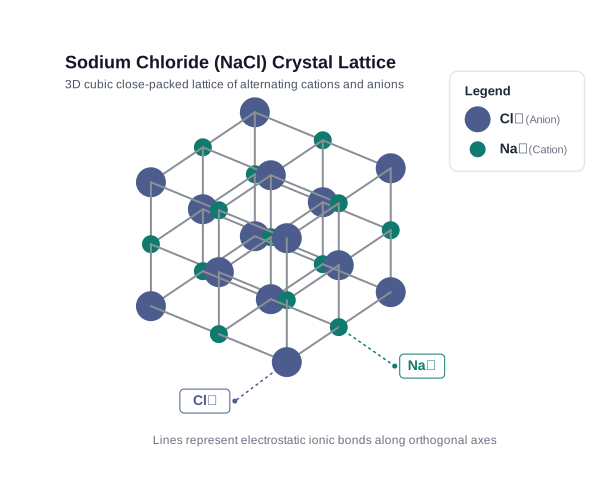
Fig. 4.9 – The rock-salt crystal structure of sodium chloride.
Here is a subtle but important point. In an ionic solid, the sum of the electron gain enthalpy and the ionization enthalpy may actually be positive (energy-costing) — and yet the crystal still forms and is stable. Why? Because a large amount of energy is released when the gaseous ions come together to build the crystal lattice.
Take sodium chloride as the worked case. The ionization enthalpy to form \(\mathrm{Na^+}\text{(g)}\) from \(\mathrm{Na}\text{(g)}\) is \(495.8\ \text{kJ mol}^{-1}\), while the electron gain enthalpy for the change \(\mathrm{Cl}\text{(g)} + \mathrm{e^-} \rightarrow \mathrm{Cl^-}\text{(g)}\) is only \(-348.7\ \text{kJ mol}^{-1}\). The sum of these two, \(147.1\ \text{kJ mol}^{-1}\), is a net energy cost. But this cost is more than compensated by the enthalpy of lattice formation of \(\mathrm{NaCl}\text{(s)}\), which is \(-788\ \text{kJ mol}^{-1}\). So the energy released in the overall process is far greater than the energy absorbed.
The lesson is a general one:
Because lattice enthalpy plays such a key role in ionic-compound formation, it is worth studying more closely.
4.2.1 Lattice Enthalpy
For example, the lattice enthalpy of \(\mathrm{NaCl}\) is \(788\ \text{kJ mol}^{-1}\). This means that \(788\ \text{kJ}\) of energy is needed to pull one mole of solid \(\mathrm{NaCl}\) apart into one mole of \(\mathrm{Na^+}\text{(g)}\) and one mole of \(\mathrm{Cl^-}\text{(g)}\), moving the ions infinitely far from one another:
\[\mathrm{NaCl}\text{(s)} \longrightarrow \mathrm{Na^+}\text{(g)} + \mathrm{Cl^-}\text{(g)} \qquad \Delta_{\text{lattice}}H = +788\ \text{kJ mol}^{-1}\]
(Notice the sign: separating the crystal costs energy, so this value is positive, whereas the reverse process of forming the lattice from ions releases the same amount, \(-788\ \text{kJ mol}^{-1}\), as used above.)
This process involves both kinds of forces at once: the attractive forces between ions of opposite charge, and the repulsive forces between ions of like charge. Because the solid crystal is three-dimensional, with every ion interacting with many neighbours, it is not possible to calculate the lattice enthalpy directly from the simple attraction–repulsion of a single pair of ions. Factors linked to the geometry of the whole crystal must also be taken into account.
4.3 Bond Parameters
Every chemical bond has a set of measurable features — how long it is, at what angle it meets its neighbours, how strong it is, how many electron pairs it involves, and how evenly the electrons are shared. These features are called bond parameters, and together they largely decide the properties of a compound.
4.3.1 Bond Length
Bond lengths are measured by spectroscopic, X-ray diffraction and electron-diffraction techniques, which you will study in higher classes. Each atom of the bonded pair contributes to the bond length, as shown in Fig. 4.10. For a covalent bond, the contribution made by each atom is called its covalent radius.
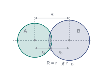
Fig. 4.10 – Bond length in a covalent molecule AB.
The covalent radius is measured, approximately, as the radius of an atom’s core when it is just in contact with the core of an adjacent bonded atom. In practice, the covalent radius is taken as half the distance between two identical atoms joined by a covalent bond in the same molecule.
A related but larger quantity is the van der Waals radius, which represents the overall size of the atom, including its valence shell, in a non-bonded situation. The van der Waals radius is half the distance between two identical atoms lying in separate molecules in a solid. The covalent and van der Waals radii of chlorine are shown in Fig. 4.11.
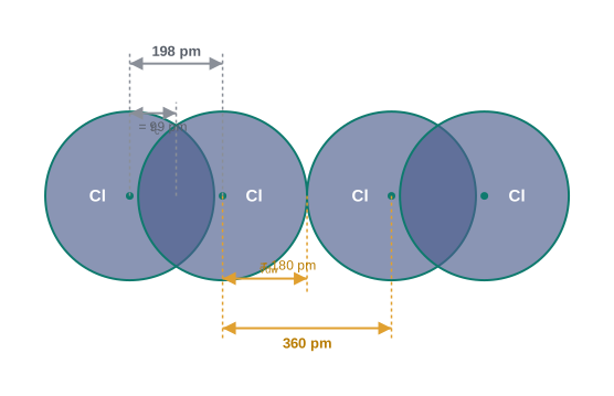
Fig. 4.11 – Covalent and van der Waals radii in chlorine.
Some typical average bond lengths for single, double and triple bonds are collected in Table 4.2, bond lengths for some common molecules in Table 4.3, and covalent radii of some common elements in Table 4.4.
Table 4.2 Average Bond Lengths for Some Single, Double and Triple Bonds
| Bond Type | Covalent Bond Length (pm) |
|---|---|
| O–H | 96 |
| C–H | 107 |
| N–O | 136 |
| C–O | 143 |
| C–N | 143 |
| C–C | 154 |
| C=O | 121 |
| N=O | 122 |
| C=C | 133 |
| C=N | 138 |
| C≡N | 116 |
| C≡C | 120 |
Table 4.3 Bond Lengths in Some Common Molecules
| Molecule | Bond Length (pm) |
|---|---|
| \(\mathrm{H_2}\) (H–H) | 74 |
| \(\mathrm{F_2}\) (F–F) | 144 |
| \(\mathrm{Cl_2}\) (Cl–Cl) | 199 |
| \(\mathrm{Br_2}\) (Br–Br) | 228 |
| \(\mathrm{I_2}\) (I–I) | 267 |
| \(\mathrm{N_2}\) (N≡N) | 109 |
| \(\mathrm{O_2}\) (O=O) | 121 |
| HF (H–F) | 92 |
| HCl (H–Cl) | 127 |
| HBr (H–Br) | 141 |
| HI (H–I) | 160 |
Table 4.4 Covalent Radii, \(r_{\text{cov}}\)/(pm)
| Element | Covalent radius (pm) |
|---|---|
| H | 37 |
| C | 77 (1), 67 (2), 60 (3) |
| N | 74 (1), 65 (2), 55 (3) |
| O | 66 (1), 57 (2) |
| F | 64 |
| Cl | 99 |
| P | 110 |
| S | 104 (1), 95 (2) |
| Br | 114 |
| As | 121 |
| Se | 104 |
| I | 133 |
| Sb | 141 |
| Te | 137 |
The values cited are for single bonds, except where otherwise indicated in parenthesis, where (1), (2) and (3) mean single, double and triple bonds respectively. (See also Chapter 3 for periodic trends.)
4.3.2 Bond Angle
Bond angle is expressed in degrees and can be found experimentally by spectroscopic methods. It tells us how the orbitals are distributed around the central atom, and therefore helps us work out the shape of the molecule. For example, the H–O–H bond angle in water is \(104.5^\circ\), as shown in Fig. 4.12.
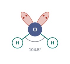
Fig. 4.12 – Bond angle in a water molecule.
4.3.3 Bond Enthalpy
The unit of bond enthalpy is \(\text{kJ mol}^{-1}\). For example, the H–H bond enthalpy in the hydrogen molecule is \(435.8\ \text{kJ mol}^{-1}\):
\[\mathrm{H_2}\text{(g)} \rightarrow \mathrm{H}\text{(g)} + \mathrm{H}\text{(g)} \qquad \Delta_a H^\circ = 435.8\ \text{kJ mol}^{-1}\]
For molecules with multiple bonds, more energy is needed to break the stronger bond. For oxygen (O=O) and nitrogen (N≡N):
\[\mathrm{O_2}\text{(g)} \rightarrow \mathrm{O}\text{(g)} + \mathrm{O}\text{(g)} \qquad \Delta_a H^\circ = 498\ \text{kJ mol}^{-1}\]
\[\mathrm{N_2}\text{(g)} \rightarrow \mathrm{N}\text{(g)} + \mathrm{N}\text{(g)} \qquad \Delta_a H^\circ = 946.0\ \text{kJ mol}^{-1}\]
The larger the bond dissociation enthalpy, the stronger is the bond in the molecule. For a heteronuclear diatomic molecule such as HCl:
\[\mathrm{HCl}\text{(g)} \rightarrow \mathrm{H}\text{(g)} + \mathrm{Cl}\text{(g)} \qquad \Delta_a H^\circ = 431.0\ \text{kJ mol}^{-1}\]
Mean bond enthalpy in polyatomic molecules
For polyatomic molecules, measuring bond strength is more complicated, because breaking successive identical bonds takes different amounts of energy. Take water, which has two O–H bonds. Breaking them one at a time gives:
\[\mathrm{H_2O}\text{(g)} \rightarrow \mathrm{H}\text{(g)} + \mathrm{OH}\text{(g)} \qquad \Delta_a H_1^\circ = 502\ \text{kJ mol}^{-1}\]
\[\mathrm{OH}\text{(g)} \rightarrow \mathrm{H}\text{(g)} + \mathrm{O}\text{(g)} \qquad \Delta_a H_2^\circ = 427\ \text{kJ mol}^{-1}\]
The difference between these two values shows that the second O–H bond breaks in a changed chemical environment, so it takes different energy. This is also why the same O–H bond has slightly different energies in different molecules, such as ethanol (\(\mathrm{C_2H_5OH}\)) and water. For such polyatomic molecules we therefore use the mean (average) bond enthalpy, obtained by dividing the total bond dissociation enthalpy by the number of bonds broken. For water:
\[\text{Average bond enthalpy} = \frac{502 + 427}{2} = 464.5\ \text{kJ mol}^{-1}\]
4.3.4 Bond Order
In the Lewis picture of a covalent bond, the bond order is simply the number of bonds between two atoms in a molecule.
Thus the bond order is 1 in \(\mathrm{H_2}\) (one shared pair), 2 in \(\mathrm{O_2}\) (two shared pairs) and 3 in \(\mathrm{N_2}\) (three shared pairs). In carbon monoxide, CO, with three shared pairs between C and O, the bond order is also 3. For \(\mathrm{N_2}\) the bond order of 3 goes with a dissociation enthalpy of \(946\ \text{kJ mol}^{-1}\) — one of the highest known for a diatomic molecule.
Isoelectronic species — those having the same number of electrons — have identical bond orders. For example, \(\mathrm{F_2}\) and \(\mathrm{O_2^{2-}}\) both have bond order 1, while \(\mathrm{N_2}\), CO and \(\mathrm{NO^+}\) all have bond order 3.
A very useful general correlation links these three parameters together: with an increase in bond order, bond enthalpy increases and bond length decreases. More shared pairs pull the nuclei closer (shorter bond) and hold them more tightly (stronger bond).
4.3.5 Resonance Structures
It is often found that a single Lewis structure cannot fully represent a molecule in agreement with its experimentally measured parameters. The ozone molecule, \(\mathrm{O_3}\), is the classic example: it can be drawn equally well as either of two Lewis structures, I and II, shown in Fig. 4.13.
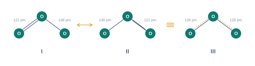
Fig. 4.13 – Canonical structures and resonance hybrid of ozone.
In both structures there is one O–O single bond and one O=O double bond. The normal O–O single-bond and O=O double-bond lengths are 148 pm and 121 pm respectively. But the experimentally measured oxygen–oxygen bond lengths in \(\mathrm{O_3}\) are both the same, 128 pm — a value intermediate between a single and a double bond. Clearly, neither of the two Lewis structures above can represent this correctly.
To deal with exactly this kind of difficulty, the concept of resonance was introduced.
Thus, for ozone, structures I and II are the canonical structures (also called resonance structures), and their hybrid — structure III — represents the real molecule more accurately. This is called the resonance hybrid. Resonance is shown by a double-headed arrow (\(\leftrightarrow\)).
Two more good examples of resonance are the carbonate ion and the carbon dioxide molecule.
Explain the structure of the \(\mathrm{CO_3^{2-}}\) ion in terms of resonance.
A single Lewis structure based on two C–O single bonds and one C=O double bond is inadequate, because it represents the three carbon–oxygen bonds as unequal. According to experiment, however, all the carbon-to-oxygen bonds in \(\mathrm{CO_3^{2-}}\) are equivalent. The carbonate ion is therefore best described as a resonance hybrid of the three canonical forms I, II and III shown in Fig. 4.14.
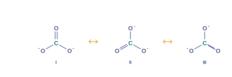
[Caption:] Fig. 4.14 – Resonance structures of the carbonate ion. [/Caption:]
Explain the structure of the \(\mathrm{CO_2}\) molecule.
The experimentally measured carbon-to-oxygen bond length in \(\mathrm{CO_2}\) is 115 pm. A normal carbon–oxygen double bond (C=O) is 121 pm and a carbon–oxygen triple bond (C≡O) is 110 pm. Since the carbon–oxygen bond lengths in \(\mathrm{CO_2}\) (115 pm) lie between the values for C=O and C≡O, a single Lewis structure cannot depict this. It becomes necessary to write more than one Lewis structure and to treat \(\mathrm{CO_2}\) as a hybrid of the canonical (resonance) forms I, II and III shown in Fig. 4.15.
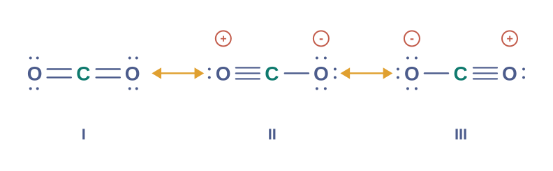
[Caption:] Fig. 4.15 – Resonance structures of carbon dioxide. [/Caption:]
In general, we can say the following about resonance:
- Resonance stabilises the molecule, because the energy of the resonance hybrid is less than the energy of any single canonical structure. (Thus the \(\mathrm{O_3}\) hybrid has lower energy than either canonical form I or II.)
- Resonance averages the bond characteristics as a whole (which is why all the C–O bonds in \(\mathrm{CO_3^{2-}}\) come out equal).
Clearing up misconceptions about resonance
Many misconceptions surround resonance, and they need to be dispelled. You should remember that:
- The canonical forms have no real existence — they are only structures we draw on paper.
- The molecule does not spend part of its time in one canonical form and part in another.
- There is no equilibrium between the canonical forms — resonance is not like the equilibrium between keto and enol forms in tautomerism.
- The molecule has a single real structure, which is the resonance hybrid, and this hybrid simply cannot be drawn as one Lewis structure.
4.3.6 Polarity of Bonds
A perfectly 100% ionic or 100% covalent bond is an idealisation. In reality, no bond — and no compound — is completely covalent or completely ionic. Even the covalent bond between two hydrogen atoms carries a trace of ionic character.
When a covalent bond forms between two identical atoms — as in \(\mathrm{H_2}\), \(\mathrm{O_2}\), \(\mathrm{Cl_2}\), \(\mathrm{N_2}\) or \(\mathrm{F_2}\) — the shared pair of electrons is attracted equally by both atoms and sits exactly midway between the two nuclei. Such a bond is a nonpolar covalent bond. In contrast, in a heteronuclear molecule such as HF, the shared pair is pulled more towards fluorine, because the electronegativity of fluorine (the power of an atom to attract shared electrons, introduced in Unit 3) is far greater than that of hydrogen. The result is a polar covalent bond.
Dipole moment
As a result of this uneven sharing (polarisation), a polar molecule possesses a dipole moment.
\[\mu = Q \times r\]
where \(Q\) is the magnitude of the charge and \(r\) is the distance of separation between the positive and negative centres.
Dipole moment is usually expressed in Debye units (D), where
\[1\ \text{D} = 3.33564 \times 10^{-30}\ \text{C m}\]
and C is the coulomb and m the metre.
Being a vector, the dipole moment is drawn as a small arrow, with its tail on the negative centre and its head pointing towards the positive centre. In chemistry, though, the presence of a dipole moment is usually marked by a crossed arrow (\(\rightarrow!!!+\)) placed on the Lewis structure, with the cross on the positive end and the arrowhead on the negative end. The dipole moment of HF is drawn this way in Fig. 4.16. Note that the direction of this crossed arrow is opposite to the conventional direction of the dipole-moment vector.
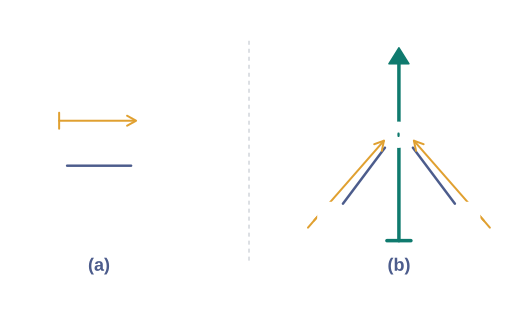
Fig. 4.16 – Dipole moments in HF and water.
For polyatomic molecules, the dipole moment depends not only on the individual bond dipoles but also on the spatial arrangement of the bonds. The molecular dipole moment is the vector sum of all the bond dipoles. For example, water has a bent structure with its two O–H bonds at \(104.5^\circ\); the resultant is a net dipole moment of \(6.17 \times 10^{-30}\ \text{C m}\), which is the vector sum of the two O–H bond dipoles:
\[\mu = 1.85\ \text{D} = 1.85 \times 3.33564 \times 10^{-30}\ \text{C m} = 6.17 \times 10^{-30}\ \text{C m}\]
The importance of geometry becomes clear when the bond dipoles cancel:
- In \(\mathrm{BeF_2}\), the dipole moment is zero, because the two equal bond dipoles point in exactly opposite directions and cancel each other.
- In \(\mathrm{BF_3}\), the dipole moment is also zero even though the B–F bonds are at \(120^\circ\) to one another; the three bond moments add up to zero, since the resultant of any two is equal and opposite to the third.
These cancellations are shown in Fig. 4.17.
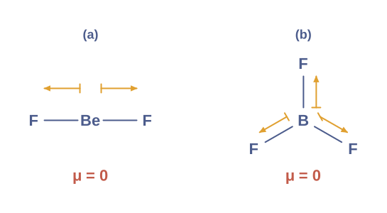
Fig. 4.17 – Cancellation of bond dipoles in BeF2 and BF3.
The special case of NH₃ and NF₃
An interesting comparison is between ammonia (\(\mathrm{NH_3}\)) and nitrogen trifluoride (\(\mathrm{NF_3}\)). Both molecules have a pyramidal shape with a lone pair of electrons on the nitrogen atom. Now, fluorine is more electronegative than nitrogen, so we might expect \(\mathrm{NF_3}\) to have the larger dipole moment. In fact the opposite is true: the dipole moment of \(\mathrm{NH_3}\) (\(4.90 \times 10^{-30}\ \text{C m}\)) is greater than that of \(\mathrm{NF_3}\) (\(0.8 \times 10^{-30}\ \text{C m}\)).
The reason lies in the direction of the orbital dipole due to the lone pair. In \(\mathrm{NH_3}\), the orbital dipole of the lone pair points in the same direction as the resultant of the three N–H bond dipoles, so the two add up. In \(\mathrm{NF_3}\), the orbital dipole of the lone pair points in the direction opposite to the resultant of the three N–F bond dipoles, so it partly cancels them, leaving \(\mathrm{NF_3}\) with a low dipole moment. This is shown in Fig. 4.18.
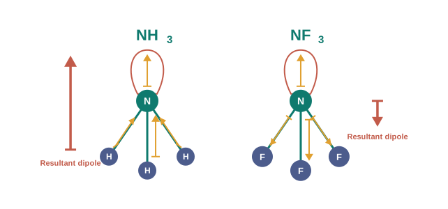
Fig. 4.18 – Comparison of dipole moments in NH3 and NF3.
The dipole moments of several molecules are collected in Table 4.5.
Table 4.5 Dipole Moments of Selected Molecules
| Type of Molecule | Example | Dipole Moment, \(\mu\) (D) | Geometry |
|---|---|---|---|
| Molecule (AB) | HF | 1.78 | linear |
| HCl | 1.07 | linear | |
| HBr | 0.79 | linear | |
| HI | 0.38 | linear | |
| \(\mathrm{H_2}\) | 0 | linear | |
| Molecule (AB₂) | \(\mathrm{H_2O}\) | 1.85 | bent |
| \(\mathrm{H_2S}\) | 0.95 | bent | |
| \(\mathrm{CO_2}\) | 0 | linear | |
| Molecule (AB₃) | \(\mathrm{NH_3}\) | 1.47 | trigonal-pyramidal |
| \(\mathrm{NF_3}\) | 0.23 | trigonal-pyramidal | |
| \(\mathrm{BF_3}\) | 0 | trigonal-planar | |
| Molecule (AB₄) | \(\mathrm{CH_4}\) | 0 | tetrahedral |
| \(\mathrm{CHCl_3}\) | 1.04 | tetrahedral | |
| \(\mathrm{CCl_4}\) | 0 | tetrahedral |
Partial covalent character of ionic bonds: Fajans’ rules
Just as every covalent bond has some partial ionic character, every ionic bond has some partial covalent character. The partial covalent character of ionic bonds was explained by Kazimierz Fajans through a set of rules:
- The smaller the size of the cation and the larger the size of the anion, the greater the covalent character of the ionic bond.
- The greater the charge on the cation, the greater the covalent character of the ionic bond.
- For cations of the same size and charge, the one with a \((n-1)d^{n},ns^{o}\) electronic configuration (typical of transition metals) is more polarising than the one with a noble-gas configuration \(ns^2np^6\) (typical of alkali and alkaline-earth metal cations).
The idea behind these rules is polarisation. The cation pulls the electron cloud of the anion towards itself, increasing the electron density between the two ions. But building up electron density between the nuclei is exactly what happens in a covalent bond. So the polarising power of the cation, the polarisability of the anion, and the extent to which the anion’s cloud is distorted together decide how much covalent character an “ionic” bond really has.
4.4 The Valence Shell Electron Pair Repulsion (VSEPR) Theory
The Lewis picture tells us which atoms are bonded and where the lone pairs sit, but it says nothing about the three-dimensional shape of a molecule. The Valence Shell Electron Pair Repulsion (VSEPR) theory fills this gap. It gives a simple procedure for predicting the shapes of covalent molecules.
The theory was first proposed by Sidgwick and Powell in 1940, based on the idea that the electron pairs in the valence shell of an atom repel one another. It was later developed and refined by Nyholm and Gillespie in 1957.
The main postulates of VSEPR theory
- The shape of a molecule depends on the number of valence-shell electron pairs — bonded and non-bonded (lone) — around the central atom.
- Pairs of electrons in the valence shell repel one another, because their electron clouds are all negatively charged.
- These electron pairs therefore arrange themselves in space so as to minimise the repulsion and maximise the distance between them.
- The valence shell is treated as a sphere, with the electron pairs sitting on its surface at maximum distance from one another.
- A multiple bond is treated as if it were a single electron pair; the two or three electron pairs of a double or triple bond are counted together as a single “super pair.”
- Where two or more resonance structures can represent a molecule, the VSEPR model can be applied to any one of them.
The last two postulates are worth pausing on. Because a double or triple bond counts as a single electron-pair region, a molecule such as \(\mathrm{SO_2}\) — which has two S=O double bonds (four bonding pairs in all) plus one lone pair — behaves as though it has just three regions around sulphur (two bond regions + one lone pair), and so comes out bent.
The order of electron-pair repulsions
Not all repulsions are equal. Nyholm and Gillespie explained the key difference between lone pairs and bonding pairs. A lone pair is localised entirely on the central atom, whereas a bonding pair is shared between two atoms and so is pulled away from the central atom. As a result, a lone pair spreads out and occupies more space than a bonding pair.
Because of this, the strength of the repulsions decreases in the order:
\[\text{lone pair–lone pair} > \text{lone pair–bond pair} > \text{bond pair–bond pair}\]
These differing repulsions push a molecule slightly away from its “ideal” shape, causing deviations in bond angles — for example, the reduction of the bond angle in ammonia and water below the perfect tetrahedral angle.
Two categories of molecules
To predict shapes, it is convenient to divide molecules into two categories:
- molecules in which the central atom has no lone pair; and
- molecules in which the central atom has one or more lone pairs.
Category 1 — central atom with no lone pair. Here the electron pairs (all bonding) arrange themselves symmetrically. Table 4.6 gives the arrangement for two to six electron pairs. The shapes are linear, trigonal planar, tetrahedral, trigonal bipyramidal and octahedral for \(\mathrm{AB_2}\), \(\mathrm{AB_3}\), \(\mathrm{AB_4}\), \(\mathrm{AB_5}\) and \(\mathrm{AB_6}\) respectively. These can be seen in molecules such as \(\mathrm{BF_3}\) (\(\mathrm{AB_3}\)), \(\mathrm{CH_4}\) (\(\mathrm{AB_4}\)) and \(\mathrm{PCl_5}\) (\(\mathrm{AB_5}\)), shown by ball-and-stick models in Fig. 4.19.
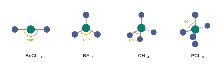
Fig. 4.19 – Shapes of molecules with no lone pairs.
Table 4.6 Geometry of Molecules in which the Central Atom has No Lone Pair of Electrons
| Number of electron pairs | Arrangement of electron pairs | Molecular geometry | Examples |
|---|---|---|---|
| 2 | Linear (180°) | Linear (B–A–B) | \(\mathrm{BeCl_2}\), \(\mathrm{HgCl_2}\) |
| 3 | Trigonal planar (120°) | Trigonal planar | \(\mathrm{BF_3}\) |
| 4 | Tetrahedral (109.5°) | Tetrahedral | \(\mathrm{CH_4}\), \(\mathrm{NH_4^+}\) |
| 5 | Trigonal bipyramidal (90°, 120°) | Trigonal bipyramidal | \(\mathrm{PCl_5}\) |
| 6 | Octahedral (90°) | Octahedral | \(\mathrm{SF_6}\) |
Category 2 — central atom with one or more lone pairs. When lone pairs are present, the molecular shape differs from the electron-pair arrangement, because we “see” only the positions of the atoms, not the lone pairs. Table 4.7 lists the shapes of some simple molecules and ions of this type, shown in Fig. 4.20. Table 4.8 then explains why the geometry is distorted and by how much the bond angles change.
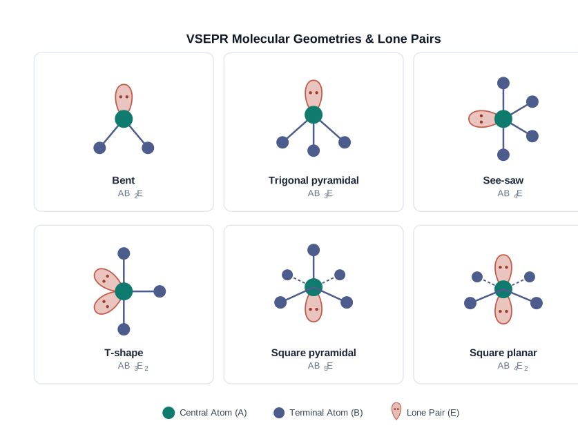
Fig. 4.20 – Shapes of molecules with lone pairs on the central atom.
Table 4.7 Shape (Geometry) of Some Simple Molecules/Ions with the Central Atom having One or More Lone Pairs of Electrons (E)
| Molecule type | Bonding pairs | Lone pairs | Arrangement of electron pairs | Shape | Example |
|---|---|---|---|---|---|
| \(\mathrm{AB_2E}\) | 2 | 1 | Trigonal planar | Bent | \(\mathrm{SO_2}\) |
| \(\mathrm{AB_3E}\) | 3 | 1 | Tetrahedral | Trigonal pyramidal | \(\mathrm{NH_3}\) |
| \(\mathrm{AB_2E_2}\) | 2 | 2 | Tetrahedral | Bent | \(\mathrm{H_2O}\) |
| \(\mathrm{AB_4E}\) | 4 | 1 | Trigonal bipyramidal | See-saw | \(\mathrm{SF_4}\) |
| \(\mathrm{AB_3E_2}\) | 3 | 2 | Trigonal bipyramidal | T-shape | \(\mathrm{ClF_3}\) |
| \(\mathrm{AB_5E}\) | 5 | 1 | Octahedral | Square pyramidal | \(\mathrm{BrF_5}\) |
| \(\mathrm{AB_4E_2}\) | 4 | 2 | Octahedral | Square planar | \(\mathrm{XeF_4}\) |
Table 4.8 Shapes of Molecules containing Bond Pair and Lone Pair
| Molecule type | Bonding pairs | Lone pairs | Shape | Reason for the shape acquired |
|---|---|---|---|---|
| \(\mathrm{AB_2E}\) | 4 | 1 | Bent | The shape should have been trigonal planar, but the lone pair–bond pair repulsion is much greater than bond pair–bond pair repulsion, so the angle is reduced to 119.5° from 120° (as in \(\mathrm{SO_2}\)). |
| \(\mathrm{AB_3E}\) | 3 | 1 | Trigonal pyramidal | Had a bond pair replaced the lone pair, the shape would be tetrahedral; but one lone pair is present, and lp–bp repulsion (greater than bp–bp) reduces the angle to 107° from 109.5° (as in \(\mathrm{NH_3}\)). |
| \(\mathrm{AB_2E_2}\) | 2 | 2 | Bent | Would be tetrahedral if all were bond pairs; but two lone pairs make it a distorted tetrahedron (angular). Since lp–lp > lp–bp > bp–bp, the angle is reduced to 104.5° from 109.5° (as in \(\mathrm{H_2O}\)). |
| \(\mathrm{AB_4E}\) | 4 | 1 | See-saw | With the lone pair in an axial position there are three lp–bp repulsions at 90°; in an equatorial position there are only two, which is more stable. The equatorial arrangement gives a distorted tetrahedron, also called a folded square or see-saw (as in \(\mathrm{SF_4}\)). |
| \(\mathrm{AB_3E_2}\) | 3 | 2 | T-shape | With both lone pairs in equatorial positions there are fewer lp–bp repulsions than when they are axial, so this arrangement is the most stable, giving a T-shape (as in \(\mathrm{ClF_3}\)). |
(Notice why the \(\mathrm{AB_2E}\) row of Table 4.8 lists four bonding pairs: \(\mathrm{SO_2}\) has two S=O double bonds, so there are four shared pairs in all, but — following the VSEPR “super-pair” rule — these count as just two bonding regions, which together with the one lone pair give the bent shape.)
How well does VSEPR theory work?
VSEPR theory is able to predict the geometry of a very large number of molecules, especially the compounds of the p-block elements, quite accurately. It is also successful even when the energy difference between possible structures is very small. Its one weakness is theoretical: the exact reason why electron-pair repulsions shape molecules the way they do is still not fully clear, and remains a subject of discussion.
4.5 Valence Bond Theory
The Lewis approach helps us write the structure of a molecule, but it fails to explain how a chemical bond actually forms. It also gives no reason for the differences in bond dissociation enthalpies and bond lengths between molecules — for example, \(\mathrm{H_2}\) (435.8 kJ mol⁻¹, 74 pm) and \(\mathrm{F_2}\) (155 kJ mol⁻¹, 144 pm) — even though both contain a single covalent bond formed by sharing one electron pair. Lewis theory gives no idea about the shapes of polyatomic molecules either.
VSEPR theory, as we have just seen, predicts the geometry of simple molecules, but it does not explain them theoretically and has limited application. To overcome these limitations, two theories based on quantum mechanics were introduced: valence bond (VB) theory and molecular orbital (MO) theory.
Valence bond theory was introduced by Heitler and London in 1927 and developed further by Pauling and others. A full treatment rests on atomic orbitals, electronic configurations (Chapter 2), the overlap of atomic orbitals, hybridisation, and the principles of variation and superposition. A rigorous mathematical treatment is beyond the scope of this book, so we discuss VB theory only in a qualitative, non-mathematical way. We begin with the simplest molecule of all — hydrogen.
Formation of the hydrogen molecule
Consider two hydrogen atoms, A and B, with nuclei \(\mathrm{N_A}\) and \(\mathrm{N_B}\) and electrons \(\mathrm{e_A}\) and \(\mathrm{e_B}\). When the atoms are far apart, there is no interaction between them. As they approach, new attractive and repulsive forces begin to operate.
Attractive forces arise between:
- the nucleus of each atom and its own electron, that is \(\mathrm{N_A}\)–\(\mathrm{e_A}\) and \(\mathrm{N_B}\)–\(\mathrm{e_B}\); and
- the nucleus of one atom and the electron of the other atom, that is \(\mathrm{N_A}\)–\(\mathrm{e_B}\) and \(\mathrm{N_B}\)–\(\mathrm{e_A}\).
Repulsive forces arise between:
- the two electrons, \(\mathrm{e_A}\)–\(\mathrm{e_B}\); and
- the two nuclei, \(\mathrm{N_A}\)–\(\mathrm{N_B}\).
The attractive forces tend to pull the two atoms together, while the repulsive forces tend to push them apart (Fig. 4.21).
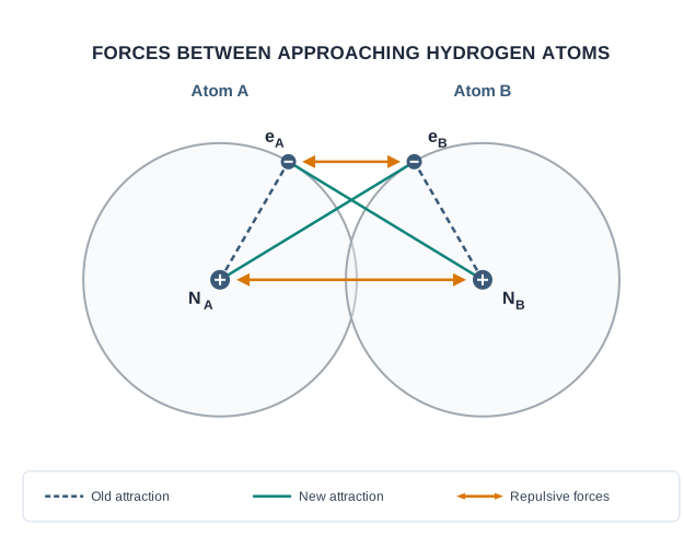
Fig. 4.21 – Forces of attraction and repulsion in H₂.
Experiment shows that the new attractive forces are stronger than the new repulsive forces. So as the atoms approach, the potential energy of the system falls. Eventually a stage is reached where the net attraction just balances the net repulsion, and the system reaches its minimum energy. At this point the two hydrogen atoms are bonded together into a stable molecule with a bond length of 74 pm.
Because energy is released when the bond forms, the hydrogen molecule is more stable than two isolated hydrogen atoms. The energy released is the bond enthalpy, and it corresponds to the minimum in the energy curve of Fig. 4.22. Conversely, the same amount of energy — 435.8 kJ — is needed to break one mole of hydrogen molecules:
\[\mathrm{H_2}\text{(g)} + 435.8\ \text{kJ mol}^{-1} \longrightarrow \mathrm{H}\text{(g)} + \mathrm{H}\text{(g)}\]
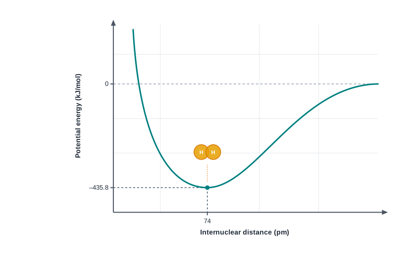
Fig. 4.22 – Potential-energy curve for H₂ formation.
4.5.1 Orbital Overlap Concept
During the formation of the hydrogen molecule, the minimum-energy state is reached when the two hydrogen atoms are so close that their atomic orbitals partly interpenetrate. This partial merging of atomic orbitals is called the overlapping of atomic orbitals, and it results in the pairing of electrons.
The extent of overlap decides the strength of the covalent bond: in general, the greater the overlap, the stronger the bond formed between two atoms.
4.5.2 Directional Properties of Bonds
As we have seen, the covalent bond is formed by the overlap of atomic orbitals. The hydrogen molecule forms by the overlap of the 1s orbitals of two H atoms.
For polyatomic molecules such as \(\mathrm{CH_4}\), \(\mathrm{NH_3}\) and \(\mathrm{H_2O}\), the geometry of the molecule matters as much as the bond formation itself. Why, for example, does \(\mathrm{CH_4}\) have a tetrahedral shape with H–C–H bond angles of 109.5°? Why is \(\mathrm{NH_3}\) pyramidal? Valence bond theory explains the shape, formation and directional properties of bonds in such molecules in terms of the overlap and hybridisation of atomic orbitals.
4.5.3 Overlapping of Atomic Orbitals
When the orbitals of two atoms come close to form a bond, their overlap may be positive, negative or zero, depending on the sign (phase) and the orientation of the orbital wave function in space (Fig. 4.23).
The positive and negative signs marked on the boundary-surface diagrams show the sign (phase) of the orbital wave function; they are not related to electric charge. (Recall that an orbital is described by a wave function, and like any wave it can have positive and negative parts.) For a bond to form, the overlapping orbitals must have the same sign (phase) and the same orientation in space — this is called positive overlap. Various overlaps of s and p orbitals are shown in Fig. 4.23.
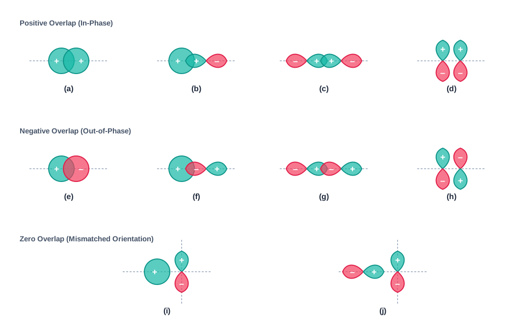
Fig. 4.23 – Overlaps of s and p atomic orbitals.
Why simple overlap alone fails to explain shape
The overlap criterion applies uniformly to homonuclear and heteronuclear diatomic molecules and to polyatomic molecules. We know that \(\mathrm{CH_4}\), \(\mathrm{NH_3}\) and \(\mathrm{H_2O}\) are tetrahedral, pyramidal and bent respectively. It is worth testing whether simple orbital overlap can explain these shapes.
Take the methane molecule, \(\mathrm{CH_4}\). The electronic configuration of carbon in its ground state is \([\mathrm{He}],2s^2,2p^2\), which in the excited state becomes \([\mathrm{He}],2s^1,2p_x^1,2p_y^1,2p_z^1\). The energy needed for this excitation is more than compensated by the energy released when carbon’s orbitals overlap with hydrogen’s.
Now, the four orbitals of carbon — each with an unpaired electron — can overlap with the singly occupied 1s orbitals of four hydrogen atoms, forming four C–H bonds. But here is the problem: the three p orbitals of carbon are mutually at 90°, so the three C–H bonds using them would be at 90° to one another. The 2s orbital of carbon and the 1s orbital of hydrogen are both spherically symmetrical and can overlap in any direction, so the direction of the fourth C–H bond cannot even be fixed.
This description does not fit the observed tetrahedral H–C–H angle of 109.5°. Clearly, simple atomic-orbital overlap fails to account for the directional character of bonds in \(\mathrm{CH_4}\). By the same argument, it wrongly predicts H–N–H and H–O–H angles of 90° for \(\mathrm{NH_3}\) and \(\mathrm{H_2O}\), in disagreement with the actual angles of 107° and 104.5°. Resolving this puzzle needs the concept of hybridisation, which is taken up in the next section.
4.5.4 Types of Overlapping and Nature of Covalent Bonds
Depending on the type of overlapping, a covalent bond is classified as either a sigma (\(\sigma\)) bond or a pi (\(\pi\)) bond.
Sigma (\(\sigma\)) bond
A sigma bond can form by any of the following combinations of atomic orbitals:
- s–s overlapping: two half-filled s orbitals overlap along the internuclear axis.
- s–p overlapping: a half-filled s orbital of one atom overlaps with a half-filled p orbital of another atom.
- p–p overlapping: half-filled p orbitals of the two approaching atoms overlap end-to-end.
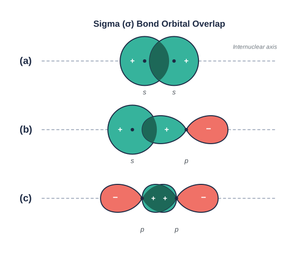
Fig. 4.24 – Sigma overlaps: (a) s–s, (b) s–p, and (c) p–p.
Pi (\(\pi\)) bond
The orbitals formed by this sidewise overlap consist of two saucer-shaped electron clouds lying above and below the plane of the participating atoms.
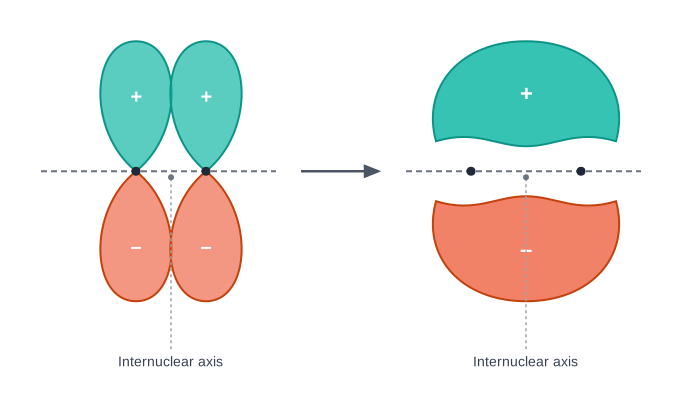
Fig. 4.25 – Formation of a pi bond.
4.5.5 Strength of Sigma and pi Bonds
The strength of a bond depends on the extent of overlapping. In a sigma bond the orbitals overlap to a larger extent, so a sigma bond is stronger. In a pi bond the overlap occurs to a smaller extent, so a pi bond is comparatively weaker.
It is also important to note that when multiple bonds form between two atoms, the pi bond(s) are always formed in addition to a sigma bond — never on their own. A double bond is one sigma + one pi; a triple bond is one sigma + two pi.
4.6 Hybridisation
At the end of the last section we hit a puzzle: simple orbital overlap predicts 90° bond angles for \(\mathrm{CH_4}\), \(\mathrm{NH_3}\) and \(\mathrm{H_2O}\), but the real angles are 109.5°, 107° and 104.5°. To explain these characteristic shapes, Pauling introduced the concept of hybridisation.
According to this idea, atomic orbitals of an atom combine to form a new set of equivalent orbitals called hybrid orbitals. Unlike the pure atomic orbitals, it is these hybrid orbitals that are used in bond formation.
Salient features of hybridisation
- The number of hybrid orbitals formed is equal to the number of atomic orbitals that get hybridised.
- The hybridised orbitals are always equivalent in energy and shape.
- The hybrid orbitals are more effective in forming stable bonds than the pure atomic orbitals.
- The hybrid orbitals are directed in space in some preferred direction so as to have minimum repulsion between electron pairs, giving a stable arrangement. Therefore, the type of hybridisation tells us the geometry of the molecule.
Important conditions for hybridisation
- The orbitals that hybridise are those present in the valence shell of the atom.
- The orbitals undergoing hybridisation should have almost equal energy.
- Promotion of an electron (excitation) is not an essential condition before hybridisation.
- It is not necessary that only half-filled orbitals take part in hybridisation; in some cases, even filled orbitals of the valence shell participate.
4.6.1 Types of Hybridisation
There are various types of hybridisation involving s, p and d orbitals. We first consider the three most common types.
(I) sp hybridisation
In \(sp\) hybridisation, one s orbital and one p orbital mix to give two equivalent \(sp\) hybrid orbitals. If the hybrids are to lie along the z-axis, the suitable orbitals are s and \(p_z\). Each \(sp\) hybrid orbital has 50% s-character and 50% p-character.
A molecule in which the central atom is \(sp\)-hybridised and linked to two other atoms has a linear geometry. For this reason \(sp\) hybridisation is also called diagonal hybridisation. The two \(sp\) hybrids point in opposite directions along the z-axis, with large positive lobes and very small negative lobes, which allows more effective overlap and hence stronger bonds.
Example — \(\mathrm{BeCl_2}\). The ground-state configuration of beryllium is \(1s^2,2s^2\). In the excited state, one 2s electron is promoted to a vacant 2p orbital, accounting for beryllium’s bivalency. One 2s and one 2p orbital then hybridise to form two \(sp\) hybrids oriented at 180° to each other. Each \(sp\) hybrid overlaps axially with a 2p orbital of chlorine, forming two Be–Cl sigma bonds, as shown in Fig. 4.26.
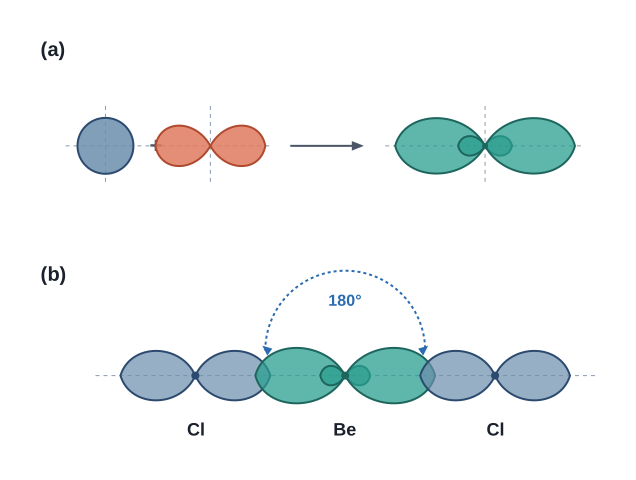
Fig. 4.26 – (a) sp hybrids and (b) BeCl₂ formation.
(II) sp² hybridisation
In \(sp^2\) hybridisation, one s orbital and two p orbitals mix to give three equivalent \(sp^2\) hybrid orbitals arranged in a trigonal planar geometry.
Example — \(\mathrm{BCl_3}\). The ground-state configuration of boron is \(1s^2,2s^2,2p^1\). In the excited state, one 2s electron is promoted to a vacant 2p orbital, giving \(1s^2,2s^1,2p^2\), so boron now has three unpaired electrons. These three orbitals (one 2s and two 2p) hybridise to form three \(sp^2\) hybrids in a trigonal planar arrangement, which overlap with 2p orbitals of chlorine to form three B–Cl bonds. Therefore, in \(\mathrm{BCl_3}\) (Fig. 4.27) the geometry is trigonal planar with a Cl–B–Cl bond angle of 120°.
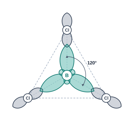
Fig. 4.27 – Formation of sp² hybrids and BCl₃.
(III) sp³ hybridisation
In \(sp^3\) hybridisation, one s orbital and three p orbitals mix to give four equivalent \(sp^3\) hybrid orbitals of equal energy and shape. Each \(sp^3\) hybrid has 25% s-character and 75% p-character. The four \(sp^3\) hybrids point towards the four corners of a tetrahedron, with an angle of 109.5° between them.
Example — \(\mathrm{CH_4}\). Taking methane, the mixing of one s orbital and three p orbitals of carbon’s valence shell gives four \(sp^3\) hybrids directed to the corners of a tetrahedron (Fig. 4.28). Each overlaps with the 1s orbital of a hydrogen atom, giving four equivalent C–H bonds at 109.5° — exactly the observed geometry.
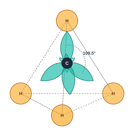
Fig. 4.28 – Formation of sp³ hybrids and CH₄.
The structures of \(\mathrm{NH_3}\) and \(\mathrm{H_2O}\) are also explained by \(sp^3\) hybridisation.
In \(\mathrm{NH_3}\), the valence-shell configuration of nitrogen in the ground state is \(2s^2,2p_x^1,2p_y^1,2p_z^1\). The four orbitals hybridise to give four \(sp^3\) hybrids: three carry the unpaired electrons and one holds a lone pair. The three half-filled hybrids overlap with the 1s orbitals of three hydrogen atoms, forming three N–H sigma bonds. Since the repulsion between a lone pair and a bond pair is greater than that between two bond pairs, the molecule is distorted and the bond angle is reduced to 107° from 109.5°, giving a pyramidal shape (Fig. 4.29).
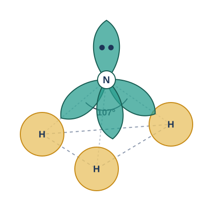
Fig. 4.29 – Pyramidal geometry of NH₃.
In \(\mathrm{H_2O}\), the four oxygen orbitals (one 2s and three 2p) undergo \(sp^3\) hybridisation to give four \(sp^3\) hybrids: two contain one electron each and the other two contain lone pairs. These four hybrids take up a tetrahedral geometry, with two corners occupied by hydrogen atoms and the other two by lone pairs. Because there are now two lone pairs, the bond angle is reduced further, to 104.5° from 109.5° (Fig. 4.30), giving water its V-shape (angular) geometry.

Fig. 4.30 – Bent geometry of H₂O.
4.6.2 Other Examples of sp³, sp² and sp Hybridisation
\(sp^3\) hybridisation in \(\mathrm{C_2H_6}\) (ethane). In ethane, both carbon atoms are \(sp^3\)-hybridised. One of the four \(sp^3\) hybrids of each carbon overlaps axially with an \(sp^3\) hybrid of the other carbon to form an \(sp^3\)–\(sp^3\) sigma bond (the C–C bond). The other three \(sp^3\) hybrids of each carbon form \(sp^3\)–s sigma bonds with hydrogen atoms. In ethane, the C–C bond length is 154 pm and each C–H bond length is 109 pm.
\(sp^2\) hybridisation in \(\mathrm{C_2H_4}\) (ethene). In ethene, one \(sp^2\) hybrid of each carbon overlaps axially with an \(sp^2\) hybrid of the other carbon to form the C–C sigma bond. The other two \(sp^2\) hybrids of each carbon form \(sp^2\)–s sigma bonds with two hydrogen atoms. The unhybridised p orbital (\(2p_x\) or \(2p_y\)) of one carbon overlaps sidewise with the similar orbital of the other carbon to form a weak \(\pi\) bond, made of two electron clouds above and below the plane of the atoms.
Thus, the carbon–carbon bond in ethene consists of one \(sp^2\)–\(sp^2\) sigma bond and one \(\pi\) bond, with a bond length of 134 pm. Each C–H bond is \(sp^2\)–s sigma with a length of 108 pm. The H–C–H bond angle is 117.6° while the H–C–C angle is 121°. The formation of the sigma and pi bonds in ethene is shown in Fig. 4.31.
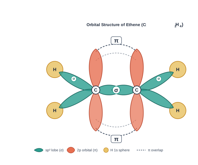
Fig. 4.31 – Sigma and pi bonds in ethene.
\(sp\) hybridisation in \(\mathrm{C_2H_2}\) (ethyne). In ethyne, both carbon atoms are \(sp\)-hybridised, each having two unhybridised p orbitals (\(2p_y\) and \(2p_x\)). One \(sp\) hybrid of each carbon overlaps axially with an \(sp\) hybrid of the other carbon to form the C–C sigma bond, while the other \(sp\) hybrid of each carbon overlaps with the half-filled s orbital of a hydrogen atom to form a σ bond. The two unhybridised p orbitals of each carbon overlap sidewise to form two π bonds between the carbon atoms. So the triple bond between the two carbon atoms is made up of one sigma bond and two pi bonds, as shown in Fig. 4.32.
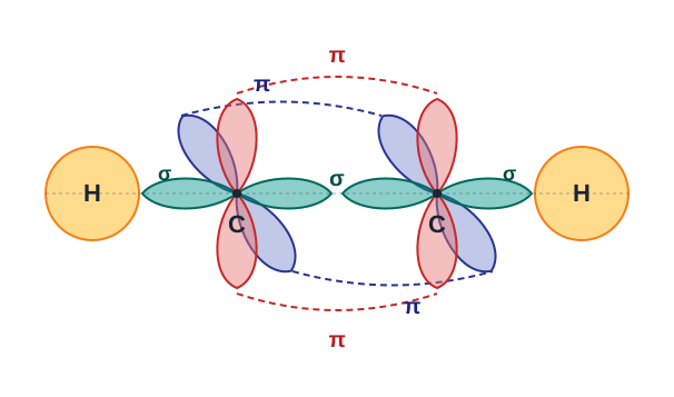
Fig. 4.32 – Sigma and pi bonds in ethyne.
4.6.3 Hybridisation of Elements involving d Orbitals
The elements of the third period have d orbitals in addition to s and p orbitals. The energy of the 3d orbitals is comparable to that of the 3s and 3p orbitals, and also comparable to that of the 4s and 4p orbitals. As a consequence, hybridisation involving either (3s, 3p, 3d) or (3d, 4s, 4p) is possible. However, because the energy difference between 3p and 4s orbitals is significant, hybridisation involving 3p, 3d and 4s together is not possible.
The important hybridisation schemes involving s, p and d orbitals are summarised below.
| Shape of molecules/ions | Hybridisation type | Atomic orbitals | Examples |
|---|---|---|---|
| Square planar | \(dsp^2\) | \(d + s + p(2)\) | \([\mathrm{Ni(CN)_4}]^{2-}\), \([\mathrm{Pt(Cl)_4}]^{2-}\) |
| Trigonal bipyramidal | \(sp^3d\) | \(s + p(3) + d\) | \(\mathrm{PF_5}\), \(\mathrm{PCl_5}\) |
| Square pyramidal | \(sp^3d^2\) | \(s + p(3) + d(2)\) | \(\mathrm{BrF_5}\) |
| Octahedral | \(sp^3d^2\) / \(d^2sp^3\) | \(s + p(3) + d(2)\) / \(d(2) + s + p(3)\) | \(\mathrm{SF_6}\), \([\mathrm{CrF_6}]^{3-}\) / \([\mathrm{Co(NH_3)_6}]^{3+}\) |
(i) Formation of PCl₅ (\(sp^3d\) hybridisation)
The ground-state outer configuration of phosphorus (\(Z = 15\)) is \(3s^2,3p^3\) with empty 3d orbitals. In the excited state, one 3s electron is promoted to a 3d orbital, giving \(3s^1,3p^3,3d^1\) with five singly occupied orbitals.
These five orbitals (one s, three p and one d) are available for hybridisation, yielding a set of five \(sp^3d\) hybrid orbitals directed towards the five corners of a trigonal bipyramidal shape, as shown in Fig. 4.33.
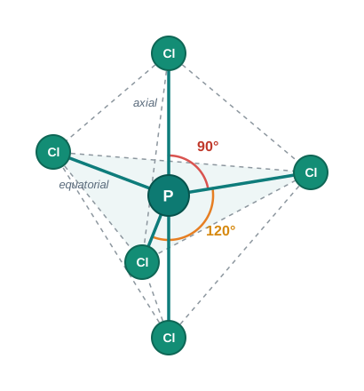
Fig. 4.33 – Trigonal bipyramidal geometry of PCl₅.
It should be noted that all the bond angles in a trigonal bipyramidal geometry are not equivalent. In \(\mathrm{PCl_5}\), the five \(sp^3d\) orbitals of phosphorus overlap with the singly occupied p orbitals of chlorine to form five P–Cl sigma bonds. Three of these P–Cl bonds lie in one plane and make angles of 120° with one another; these are the equatorial bonds. The remaining two P–Cl bonds — one above and one below the equatorial plane — make angles of 90° with the plane; these are the axial bonds.
Because the axial bond pairs suffer more repulsion from the equatorial bond pairs, the axial bonds are found to be slightly longer, and hence slightly weaker, than the equatorial bonds. This is what makes the \(\mathrm{PCl_5}\) molecule more reactive.
(ii) Formation of SF₆ (\(sp^3d^2\) hybridisation)
In \(\mathrm{SF_6}\), the central sulphur atom has the ground-state outer configuration \(3s^2,3p^4\). In the excited state, six orbitals (one s, three p and two d) become singly occupied. These orbitals hybridise to form six new \(sp^3d^2\) hybrid orbitals, projected towards the six corners of a regular octahedron.
These six \(sp^3d^2\) hybrids overlap with the singly occupied orbitals of six fluorine atoms to form six S–F sigma bonds. Thus the \(\mathrm{SF_6}\) molecule has a regular octahedral geometry, as shown in Fig. 4.34.
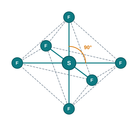
Fig. 4.34 – Octahedral geometry of SF₆.
4.7 Molecular Orbital Theory
Valence bond theory pictures a bond as the overlap of atomic orbitals that still belong to their own atoms. Molecular orbital (MO) theory takes a bolder view: it treats the electrons as belonging to the whole molecule, spread across new orbitals that span all the nuclei. MO theory was developed by F. Hund and R. S. Mulliken in 1932.
Salient features of MO theory
- The electrons in a molecule are present in various molecular orbitals, just as the electrons of an atom are present in various atomic orbitals.
- The atomic orbitals of comparable energy and proper symmetry combine to form molecular orbitals.
- An electron in an atomic orbital is influenced by one nucleus (the orbital is monocentric), whereas an electron in a molecular orbital is influenced by two or more nuclei (the orbital is polycentric).
- The number of molecular orbitals formed equals the number of combining atomic orbitals. When two atomic orbitals combine, two molecular orbitals form — one bonding molecular orbital and one antibonding molecular orbital.
- The bonding molecular orbital has lower energy, and therefore greater stability, than the corresponding antibonding molecular orbital.
- Just as an atomic orbital gives the electron probability distribution around a single nucleus, a molecular orbital gives the electron probability distribution around a group of nuclei in a molecule.
- Molecular orbitals, like atomic orbitals, are filled following the Aufbau principle, the Pauli exclusion principle and Hund’s rule.
4.7.1 Formation of Molecular Orbitals — Linear Combination of Atomic Orbitals (LCAO)
According to wave mechanics, atomic orbitals are described by wave functions (\(\psi\)), which represent the amplitude of the electron waves. These come from the solution of the Schrödinger wave equation. But the equation cannot be solved exactly for any system with more than one electron, so molecular orbitals are hard to obtain directly. To get around this, an approximate method called the linear combination of atomic orbitals (LCAO) is used.
Apply this to the hydrogen molecule. Each hydrogen atom (A and B) has one electron in a 1s orbital, described by the wave functions \(\psi_A\) and \(\psi_B\). The molecular orbitals are formed by the linear combination — the addition and subtraction — of these atomic wave functions:
\[\psi_{\text{MO}} = \psi_A \pm \psi_B\]
This gives the two molecular orbitals \(\sigma\) and \(\sigma^*\):
\[\sigma = \psi_A + \psi_B\]
\[\sigma^* = \psi_A - \psi_B\]
The molecular orbital \(\sigma\), formed by the addition of atomic orbitals, is the bonding molecular orbital, while the molecular orbital \(\sigma^*\), formed by the subtraction, is the antibonding molecular orbital, as shown in Fig. 4.35.
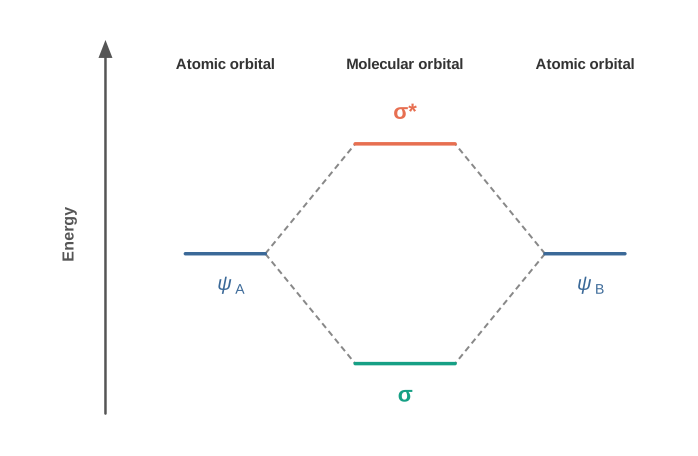
Fig. 4.35 – Formation of bonding and antibonding MOs.
Qualitatively, the two combinations can be understood as interference of the electron waves. In the bonding molecular orbital, the two electron waves reinforce each other by constructive interference. In the antibonding molecular orbital, the two waves cancel each other by destructive interference.
The consequences are important. In a bonding MO, the electron density is concentrated between the nuclei, so the repulsion between the nuclei is very low. In an antibonding MO, most of the electron density lies away from the space between the nuclei; in fact there is a nodal plane (a plane on which the electron density is zero) between the nuclei, so the nuclei repel each other strongly.
Electrons in a bonding MO therefore help hold the nuclei together and stabilise the molecule, so a bonding MO always has lower energy than either of the atomic orbitals that formed it. Electrons in an antibonding MO destabilise the molecule, because their mutual repulsion outweighs their attraction to the nuclei, causing a net increase in energy.
It is worth noting that the antibonding orbital is raised above the parent atomic orbitals by the same amount that the bonding orbital is lowered below them, so the total energy of the two molecular orbitals equals that of the two original atomic orbitals.
4.7.2 Conditions for the Combination of Atomic Orbitals
The linear combination of atomic orbitals into molecular orbitals happens only if three conditions are met.
1. The combining atomic orbitals must have the same or nearly the same energy. For example, a 1s orbital of one atom can combine with a 1s orbital of another, but not with a 2s orbital, because the energy of the 2s orbital is appreciably higher than that of the 1s. (This restriction relaxes if the two atoms are very different.)
2. The combining atomic orbitals must have the same symmetry about the molecular axis. By convention the z-axis is taken as the molecular axis. Atomic orbitals of the same energy will not combine if they have different symmetry. For example, the \(2p_z\) orbital of one atom can combine with the \(2p_z\) orbital of the other, but not with the \(2p_x\) or \(2p_y\) orbitals, because these have different symmetries.
3. The combining atomic orbitals must overlap to the maximum extent. The greater the overlap, the greater the electron density between the nuclei of the resulting molecular orbital.
4.7.3 Types of Molecular Orbitals
Molecular orbitals of diatomic molecules are designated as \(\sigma\) (sigma), \(\pi\) (pi), \(\delta\) (delta), and so on.
In this naming, the sigma (\(\sigma\)) molecular orbitals are symmetrical about the bond axis, while the pi (\(\pi\)) molecular orbitals are not symmetrical. For example, the linear combination of 1s orbitals on two nuclei gives two molecular orbitals that are symmetrical about the bond axis; these are of the \(\sigma\) type and are designated \(\sigma 1s\) and \(\sigma^* 1s\) (Fig. 4.36(a)).
Taking the internuclear axis along the z-direction, a linear combination of the \(2p_z\) orbitals of two atoms also gives two sigma molecular orbitals, designated \(\sigma 2p_z\) and \(\sigma^* 2p_z\) (Fig. 4.36(b)).
The molecular orbitals obtained from the \(2p_x\) and \(2p_y\) orbitals are not symmetrical about the bond axis, because they have positive lobes above and negative lobes below the molecular plane. These are labelled \(\pi\) and \(\pi^*\) (Fig. 4.36(c)). A \(\pi\) bonding MO has a larger electron density above and below the internuclear axis, whereas the \(\pi^*\) antibonding MO has a node between the nuclei.
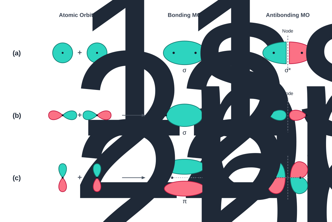
Fig. 4.36 – Contours of bonding and antibonding MOs.
4.7.4 Energy Level Diagram for Molecular Orbitals
The 1s atomic orbitals on two atoms give two molecular orbitals, \(\sigma 1s\) and \(\sigma^* 1s\). In the same way, the 2s and 2p atomic orbitals (eight atomic orbitals on the two atoms together) give rise to the following eight molecular orbitals:
- Antibonding MOs: \(\sigma^* 2s\), \(\sigma^* 2p_z\), \(\pi^* 2p_x\), \(\pi^* 2p_y\)
- Bonding MOs: \(\sigma 2s\), \(\sigma 2p_z\), \(\pi 2p_x\), \(\pi 2p_y\)
The energy levels of these molecular orbitals have been found experimentally from spectroscopic data for the homonuclear diatomic molecules of the second-row elements. For \(\mathrm{O_2}\) and \(\mathrm{F_2}\), the increasing order of energy is:
\[\sigma 1s < \sigma^* 1s < \sigma 2s < \sigma^* 2s < \sigma 2p_z < (\pi 2p_x = \pi 2p_y) < (\pi^* 2p_x = \pi^* 2p_y) < \sigma^* 2p_z\]
However, this order is not correct for the lighter molecules \(\mathrm{Li_2}\), \(\mathrm{Be_2}\), \(\mathrm{B_2}\), \(\mathrm{C_2}\) and \(\mathrm{N_2}\). It has been observed experimentally that for molecules such as \(\mathrm{B_2}\), \(\mathrm{C_2}\) and \(\mathrm{N_2}\), the increasing order of energy is:
\[\sigma 1s < \sigma^* 1s < \sigma 2s < \sigma^* 2s < (\pi 2p_x = \pi 2p_y) < \sigma 2p_z < (\pi^* 2p_x = \pi^* 2p_y) < \sigma^* 2p_z\]
The key difference in this second order is that the energy of the \(\sigma 2p_z\) molecular orbital is higher than that of the \(\pi 2p_x\) and \(\pi 2p_y\) molecular orbitals. (This reordering, caused by mixing between 2s and 2p orbitals, matters when we write the configurations of \(\mathrm{B_2}\), \(\mathrm{C_2}\) and \(\mathrm{N_2}\) in the next section.)
4.7.5 Electronic Configuration and Molecular Behaviour
The distribution of electrons among the various molecular orbitals is called the electronic configuration of the molecule. From it we can read off several important properties.
Stability of molecules
Let \(N_b\) be the number of electrons in bonding orbitals and \(N_a\) the number in antibonding orbitals. Then:
- the molecule is stable if \(N_b\) is greater than \(N_a\); and
- the molecule is unstable if \(N_b\) is less than \(N_a\).
In case (i) more bonding orbitals are occupied, so the bonding influence is stronger and a stable molecule results. In case (ii) the antibonding influence is stronger, so the molecule is unstable.
Bond order
\[\text{Bond order} = \frac{1}{2},(N_b - N_a)\]
The stability rule can now be restated in terms of bond order: a positive bond order (\(N_b > N_a\)) means a stable molecule, while a negative (\(N_b < N_a\)) or zero (\(N_b = N_a\)) bond order means an unstable molecule.
Nature of the bond. Integral bond order values of 1, 2 or 3 correspond to single, double and triple bonds respectively, matching the classical idea.
Bond length. The bond order between two atoms is an approximate measure of the bond length: the bond length decreases as the bond order increases.
Magnetic nature
If all the molecular orbitals in a molecule are doubly occupied (all electrons paired), the substance is diamagnetic — it is weakly repelled by a magnetic field. However, if one or more molecular orbitals are singly occupied (unpaired electrons present), the substance is paramagnetic — it is attracted by a magnetic field. The oxygen molecule, \(\mathrm{O_2}\), is the classic example of a paramagnetic molecule.
4.8 Bonding in Some Homonuclear Diatomic Molecules
We now apply molecular orbital theory to some homonuclear diatomic molecules (molecules made of two identical atoms). For each one we fill the electrons into the molecular orbitals in order of increasing energy, write the electronic configuration, and then read off the bond order and magnetic behaviour.
Hydrogen molecule (H₂)
The hydrogen molecule is formed by combining two hydrogen atoms, each with one electron in a 1s orbital. There are therefore two electrons in all, both going into the \(\sigma 1s\) molecular orbital. The electronic configuration of the hydrogen molecule is:
\[\mathrm{H_2}: (\sigma 1s)^2\]
Its bond order is:
\[\text{Bond order} = \frac{N_b - N_a}{2} = \frac{2 - 0}{2} = 1\]
So the two hydrogen atoms are bonded by a single covalent bond. The bond dissociation energy of the hydrogen molecule has been found to be \(438\ \text{kJ mol}^{-1}\) and the bond length is 74 pm. Since there is no unpaired electron, \(\mathrm{H_2}\) is diamagnetic.
Helium molecule (He₂)
The electronic configuration of a helium atom is \(1s^2\). Each helium atom has 2 electrons, so the \(\mathrm{He_2}\) molecule would have 4 electrons, filling both the \(\sigma 1s\) and \(\sigma^* 1s\) molecular orbitals:
\[\mathrm{He_2}: (\sigma 1s)^2 (\sigma^* 1s)^2\]
Its bond order is:
\[\text{Bond order} = \frac{1}{2}(2 - 2) = 0\]
A zero bond order means the \(\mathrm{He_2}\) molecule is unstable and does not exist. In the same way, it can be shown that the \(\mathrm{Be_2}\) molecule, with configuration \((\sigma 1s)^2 (\sigma^* 1s)^2 (\sigma 2s)^2 (\sigma^* 2s)^2\), also does not exist (bond order zero).
Lithium molecule (Li₂)
The electronic configuration of lithium is \(1s^2,2s^1\), so there are six electrons in \(\mathrm{Li_2}\). Its molecular electronic configuration is:
\[\mathrm{Li_2}: (\sigma 1s)^2 (\sigma^* 1s)^2 (\sigma 2s)^2\]
This is also written as \(KK(\sigma 2s)^2\), where \(KK\) represents the filled K-shell part \((\sigma 1s)^2 (\sigma^* 1s)^2\).
Here four electrons occupy bonding orbitals and two occupy antibonding orbitals, so the bond order is \(\tfrac{1}{2}(4-2) = 1\). This means \(\mathrm{Li_2}\) is stable, and since it has no unpaired electrons, it should be diamagnetic. Diamagnetic \(\mathrm{Li_2}\) molecules are indeed known to exist in the vapour phase.
Carbon molecule (C₂)
The electronic configuration of carbon is \(1s^2,2s^2,2p^2\), so there are twelve electrons in \(\mathrm{C_2}\). Its molecular electronic configuration is:
\[\mathrm{C_2}: (\sigma 1s)^2 (\sigma^* 1s)^2 (\sigma 2s)^2 (\sigma^* 2s)^2 (\pi 2p_x^2 = \pi 2p_y^2)\]
or, in the short form:
\[\mathrm{C_2}: KK(\sigma 2s)^2 (\sigma^* 2s)^2 (\pi 2p_x^2 = \pi 2p_y^2)\]
The bond order of \(\mathrm{C_2}\) is \(\tfrac{1}{2}(8-4) = 2\), and \(\mathrm{C_2}\) should be diamagnetic. Diamagnetic \(\mathrm{C_2}\) molecules have indeed been detected in the vapour phase.
An interesting point: the double bond in \(\mathrm{C_2}\) consists of both pi bonds, because the four electrons sit in two pi molecular orbitals. In most other molecules a double bond is made of one sigma and one pi bond. In a similar way, the bonding in the \(\mathrm{N_2}\) molecule can be discussed (it has a bond order of 3, as noted earlier).
Oxygen molecule (O₂)
The electronic configuration of an oxygen atom is \(1s^2,2s^2,2p^4\), so each oxygen atom has 8 electrons and the \(\mathrm{O_2}\) molecule has 16 electrons in all. Its molecular electronic configuration is:
\[\mathrm{O_2}: (\sigma 1s)^2 (\sigma^* 1s)^2 (\sigma 2s)^2 (\sigma^* 2s)^2 (\sigma 2p_z)^2 (\pi 2p_x^2 \equiv \pi 2p_y^2)(\pi^* 2p_x^1 \equiv \pi^* 2p_y^1)\]
From this configuration, ten electrons occupy bonding molecular orbitals and six occupy antibonding molecular orbitals. Its bond order is therefore:
\[\text{Bond order} = \frac{1}{2}[N_b - N_a] = \frac{1}{2}[10 - 6] = 2\]
So in oxygen the atoms are held by a double bond. Crucially, the configuration also shows two unpaired electrons, one each in the \(\pi^* 2p_x\) and \(\pi^* 2p_y\) molecular orbitals. This means \(\mathrm{O_2}\) should be paramagnetic — a prediction that matches experiment. In this way, molecular orbital theory successfully explains the paramagnetic nature of oxygen, something the simple Lewis picture cannot do.
Molecular orbital data for B₂ through Ne₂
The electronic configurations of the other second-row homonuclear diatomic molecules can be written in the same way. The molecular-orbital occupancy and molecular properties for \(\mathrm{B_2}\) through \(\mathrm{Ne_2}\) are summarised in Fig. 4.37; the bond energy, bond length, bond order, magnetic properties and valence electron configuration are collected in Table 4.9 below. Note the change: \(\mathrm{B_2}\), \(\mathrm{C_2}\) and \(\mathrm{N_2}\) follow the order with 2s–2p mixing, while \(\mathrm{O_2}\), \(\mathrm{F_2}\) and \(\mathrm{Ne_2}\) follow the order without 2s–2p mixing.

Fig. 4.37 – Molecular-orbital occupancy for B₂ through Ne₂.
Table 4.9 Molecular Properties of B₂ through Ne₂
| Property | \(\mathrm{B_2}\) | \(\mathrm{C_2}\) | \(\mathrm{N_2}\) | \(\mathrm{O_2}\) | \(\mathrm{F_2}\) | \(\mathrm{Ne_2}\) |
|---|---|---|---|---|---|---|
| Bond energy (kJ mol⁻¹) | 290 | 620 | 945 | 498 | 159 | — |
| Bond length (pm) | 159 | 131 | 110 | 121 | 143 | — |
| Bond order | 1 | 2 | 3 | 2 | 1 | 0 |
| Magnetic property | Paramagnetic | Diamagnetic | Diamagnetic | Paramagnetic | Diamagnetic | — |
| Valence electron configuration | \((\sigma 2s)^2(\sigma^* 2s)^2(\pi 2p)^2\) | \((\sigma 2s)^2(\sigma^* 2s)^2(\pi 2p)^4\) | \((\sigma 2s)^2(\sigma^* 2s)^2(\pi 2p)^4(\sigma 2p)^2\) | \((\sigma 2s)^2(\sigma^* 2s)^2(\sigma 2p)^2(\pi 2p)^4(\pi^* 2p)^2\) | \((\sigma 2s)^2(\sigma^* 2s)^2(\sigma 2p)^2(\pi 2p)^4(\pi^* 2p)^4\) | \((\sigma 2s)^2(\sigma^* 2s)^2(\sigma 2p)^2(\pi 2p)^4(\pi^* 2p)^4(\sigma^* 2p)^2\) |
Reading across the table shows the theory’s power: bond order rises to a maximum of 3 at \(\mathrm{N_2}\) (the shortest, strongest bond), then falls, and reaches 0 at \(\mathrm{Ne_2}\) — which is why \(\mathrm{Ne_2}\) does not exist. The paramagnetic molecules \(\mathrm{B_2}\) and \(\mathrm{O_2}\) are exactly those with unpaired electrons.
4.9 Hydrogen Bonding
Nitrogen, oxygen and fluorine are among the most electronegative elements. When one of them is attached to a hydrogen atom by a covalent bond, the shared electrons are pulled strongly towards the more electronegative atom. This leaves the hydrogen atom partially positive, and it can then form a weak bond with another electronegative atom nearby. This bond is called a hydrogen bond, and it is weaker than a covalent bond.
For example, in hydrogen fluoride the hydrogen bond exists between the hydrogen atom of one HF molecule and the fluorine atom of a neighbouring molecule:
\[-,-,-,\mathrm{H^{\delta+}}!—!\mathrm{F^{\delta-}},-,-,-,\mathrm{H^{\delta+}}!—!\mathrm{F^{\delta-}},-,-,-,\mathrm{H^{\delta+}}!—!\mathrm{F^{\delta-}}\]
Here the hydrogen bond acts as a bridge between two atoms: it holds one atom by a covalent bond and the other by a hydrogen bond. By convention, the hydrogen bond is drawn as a dotted line (\(-,-,-\)), while a solid line represents the covalent bond.
4.9.1 Cause of Formation of Hydrogen Bond
When hydrogen is bonded to a strongly electronegative element ‘X’, the electron pair shared between the two atoms is pulled far away from the hydrogen atom. As a result, the hydrogen atom becomes highly electropositive with respect to ‘X’.
Because of this displacement of electrons towards X, the hydrogen acquires a fractional positive charge (\(\delta^+\)), while X gains a fractional negative charge (\(\delta^-\)). This produces a polar molecule, and the electrostatic attraction between the \(\delta^+\) hydrogen of one molecule and the \(\delta^-\) atom of the next can be represented as:
\[\mathrm{H^{\delta+}}!—!\mathrm{X^{\delta-}},-,-,-,\mathrm{H^{\delta+}}!—!\mathrm{X^{\delta-}},-,-,-,\mathrm{H^{\delta+}}!—!\mathrm{X^{\delta-}}\]
The magnitude of hydrogen bonding depends on the physical state of the compound. It is maximum in the solid state and minimum in the gaseous state. Because of this, hydrogen bonds have a strong influence on the structure and properties of compounds. (In strength, a hydrogen bond lies in between: it is much weaker than a covalent bond, but noticeably stronger than an ordinary van der Waals force of attraction.)
4.9.2 Types of Hydrogen Bonds
There are two types of hydrogen bonds.
(1) Intermolecular hydrogen bond
An intermolecular hydrogen bond is formed between two different molecules of the same compound or of different compounds. Examples include the hydrogen bonds in hydrogen fluoride, in alcohols, and in water.
(2) Intramolecular hydrogen bond
An intramolecular hydrogen bond is formed when the hydrogen atom lies between two highly electronegative (F, O, N) atoms present within the same molecule. For example, in o-nitrophenol the hydrogen is bonded between the two oxygen atoms of the same molecule, as shown in Fig. 4.38.
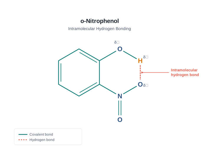
Fig. 4.38 – Intramolecular hydrogen bonding in o-nitrophenol.
4.10 Summary
- Electrovalency (Kössel’s insight). Kössel linked the formation of positive and negative ions to the atoms attaining stable noble-gas configurations. The electrostatic attraction between the oppositely charged ions is the cause of their stability, and this gives the concept of electrovalency (the ionic bond).
- Covalent bonding (Lewis’s insight). Lewis described covalent bonding as the sharing of electron pairs between atoms so that each attains a noble-gas configuration. Lewis dot symbols show the number of valence electrons of an element, while Lewis dot structures give a pictorial representation of bonding in molecules.
- Ionic crystals. An ionic compound is a three-dimensional, ordered aggregation of positive and negative ions called the crystal lattice, with an overall balance of charge. The lattice is stabilised by the enthalpy of lattice formation, which is the real measure of an ionic compound’s stability.
- Bonds and bond parameters. A single covalent bond shares one electron pair; multiple bonds share two or three pairs. Electron pairs not used in bonding are lone pairs. A Lewis structure shows the bonded pairs and lone pairs around each atom. The key bond parameters — bond length, bond angle, bond enthalpy, bond order and bond polarity — strongly affect the properties of compounds.
- Resonance. When a single Lewis structure cannot describe a molecule or ion accurately, several structures (canonical forms) with the same skeleton are drawn, and together they represent the real species. This is the concept of resonance, and the canonical forms taken together make up the resonance hybrid.
- VSEPR model. The shapes of molecules are predicted by assuming that valence-shell electron pairs repel one another and stay as far apart as possible. Molecular geometry is decided by the repulsions between lone pairs and lone pairs, between lone pairs and bonding pairs, and between bonding pairs and bonding pairs, in the order: lp–lp > lp–bp > bp–bp.
- Valence bond (VB) approach. VB theory deals with the energetics of bond formation, about which the Lewis and VSEPR models are silent. A bond forms by the overlap of atomic orbitals — for example, \(\mathrm{H_2}\) forms by the overlap of the two singly occupied 1s orbitals. As the atoms approach, the potential energy falls to a minimum at the equilibrium bond distance; pushing the nuclei closer raises the energy sharply and destabilises the molecule. Overlap increases the electron density between the nuclei, though the exact bond enthalpy and bond length depend on more than overlap alone.
- Hybridisation. To explain the shapes of polyatomic molecules, Pauling introduced hybridisation. The \(sp\), \(sp^2\) and \(sp^3\) hybridisations of the atomic orbitals of Be, B, C, N and O explain the formation and shapes of \(\mathrm{BeCl_2}\), \(\mathrm{BCl_3}\), \(\mathrm{CH_4}\), \(\mathrm{NH_3}\) and \(\mathrm{H_2O}\), as well as the multiple bonds in \(\mathrm{C_2H_2}\) and \(\mathrm{C_2H_4}\).
- Molecular orbital (MO) theory. MO theory describes bonding by combining atomic orbitals into molecular orbitals that belong to the whole molecule. The number of molecular orbitals equals the number of atomic orbitals combined. Bonding MOs increase electron density between the nuclei and are lower in energy than the atomic orbitals; antibonding MOs have a region of zero electron density between the nuclei and are higher in energy. Electrons fill the molecular orbitals in order of increasing energy, following the Aufbau principle, the Pauli exclusion principle and Hund’s rule. A molecule is stable when the number of electrons in bonding orbitals exceeds those in antibonding orbitals.
- Hydrogen bond. A hydrogen bond forms when a hydrogen atom lies between two highly electronegative atoms such as F, O and N. It may be intermolecular (between two or more molecules) or intramolecular (within one molecule). Hydrogen bonds have a powerful effect on the structure and properties of many compounds.
Flowchart
Fig. 4.39 – Evolution of the models of chemical bonding covered in this chapter: Kössel–Lewis approach (octet rule → ionic bond by electron transfer, covalent bond by electron sharing, Lewis structures, formal charge) → bond parameters (length, angle, enthalpy, order, resonance, polarity) → VSEPR theory (shapes from electron-pair repulsions) → Valence Bond theory (bonding by orbital overlap; σ and π bonds) → Hybridisation (sp, sp², sp³, sp³d, sp³d²) → Molecular Orbital theory (bonding/antibonding MOs, bond order, magnetism) → Hydrogen bonding (intermolecular and intramolecular).
Key relations to remember
- Formal charge on an atom: \(\text{F.C.} = N_{\text{v}} - N_{\text{n}} - \tfrac{1}{2}N_{\text{b}}\) (valence electrons − lone-pair electrons − half the bonding electrons).
- Dipole moment: \(\mu = Q \times r\), expressed in debye, with \(1\ \text{D} = 3.33564 \times 10^{-30}\ \text{C m}\).
- Bond order (MO theory): \(\text{Bond order} = \tfrac{1}{2}(N_b - N_a)\); a positive value means a stable molecule, and bond length decreases as bond order increases.
4.11 NCERT Questions
- Explain the formation of a chemical bond.
- Write Lewis dot symbols for atoms of the following elements: Mg, Na, B, O, N, Br.
- Write Lewis symbols for the following atoms and ions: S and \(\mathrm{S^{2-}}\); Al and \(\mathrm{Al^{3+}}\); H and \(\mathrm{H^-}\).
- Draw the Lewis structures for the following molecules and ions: \(\mathrm{H_2S}\), \(\mathrm{SiCl_4}\), \(\mathrm{BeF_2}\), \(\mathrm{CO_3^{2-}}\), HCOOH.
- Define octet rule. Write its significance and limitations.
- Write the favourable factors for the formation of an ionic bond.
- Discuss the shape of the following molecules using the VSEPR model: \(\mathrm{BeCl_2}\), \(\mathrm{BCl_3}\), \(\mathrm{SiCl_4}\), \(\mathrm{AsF_5}\), \(\mathrm{H_2S}\), \(\mathrm{PH_3}\).
- Although the geometries of \(\mathrm{NH_3}\) and \(\mathrm{H_2O}\) molecules are distorted tetrahedral, the bond angle in water is less than that of ammonia. Discuss.
- How do you express the bond strength in terms of bond order?
- Define the bond length.
- Explain the important aspects of resonance with reference to the \(\mathrm{CO_3^{2-}}\) ion.
- \(\mathrm{H_3PO_3}\) can be represented by structures 1 and 2 shown in Fig. 4.40. Can these two structures be taken as the canonical forms of the resonance hybrid representing \(\mathrm{H_3PO_3}\)? If not, give reasons for the same.
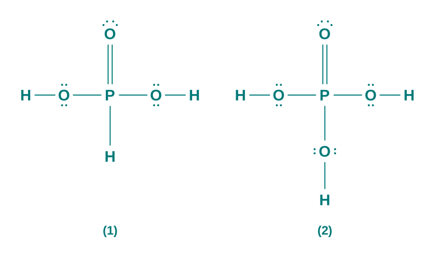
Fig. 4.40 – Lewis structures of H₃PO₃.
- Write the resonance structures for \(\mathrm{SO_3}\), \(\mathrm{NO_2}\) and \(\mathrm{NO_3^-}\).
- Use Lewis symbols to show electron transfer between the following atoms to form cations and anions:
- K and S
- Ca and O
- Al and N.
- Although both \(\mathrm{CO_2}\) and \(\mathrm{H_2O}\) are triatomic molecules, the shape of the \(\mathrm{H_2O}\) molecule is bent while that of \(\mathrm{CO_2}\) is linear. Explain this on the basis of dipole moment.
- Write the significance/applications of dipole moment.
- Define electronegativity. How does it differ from electron gain enthalpy?
- Explain, with the help of a suitable example, a polar covalent bond.
- Arrange the bonds in order of increasing ionic character in the molecules: LiF, \(\mathrm{K_2O}\), \(\mathrm{N_2}\), \(\mathrm{SO_2}\) and \(\mathrm{ClF_3}\).
- The skeletal structure of \(\mathrm{CH_3COOH}\) as shown in Fig. 4.41 is correct, but some of the bonds are shown incorrectly. Write the correct Lewis structure for acetic acid.
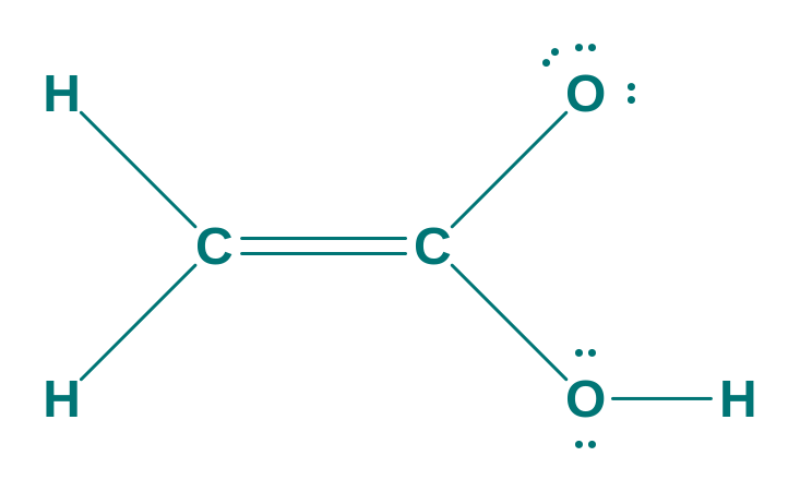
Fig. 4.41 – Incorrect skeletal structure of CH₃COOH.
- Apart from tetrahedral geometry, another possible geometry for \(\mathrm{CH_4}\) is square planar, with the four H atoms at the corners of the square and the C atom at its centre. Explain why \(\mathrm{CH_4}\) is not square planar.
- Explain why the \(\mathrm{BeH_2}\) molecule has a zero dipole moment although the Be–H bonds are polar.
- Which out of \(\mathrm{NH_3}\) and \(\mathrm{NF_3}\) has the higher dipole moment and why?
- What is meant by hybridisation of atomic orbitals? Describe the shapes of \(sp\), \(sp^2\) and \(sp^3\) hybrid orbitals.
- Describe the change in hybridisation (if any) of the Al atom in the following reaction: \[\mathrm{AlCl_3} + \mathrm{Cl^-} \rightarrow \mathrm{AlCl_4^-}\]
- Is there any change in the hybridisation of B and N atoms as a result of the following reaction? \[\mathrm{BF_3} + \mathrm{NH_3} \rightarrow \mathrm{F_3B!\cdot!NH_3}\]
- Draw diagrams showing the formation of a double bond and a triple bond between carbon atoms in \(\mathrm{C_2H_4}\) and \(\mathrm{C_2H_2}\) molecules.
- What is the total number of sigma and pi bonds in the following molecules?
- \(\mathrm{C_2H_2}\)
- \(\mathrm{C_2H_4}\).
- Considering the x-axis as the internuclear axis, which out of the following will not form a sigma bond and why?
- 1s and 1s
- 1s and \(2p_x\)
- \(2p_y\) and \(2p_y\)
- 1s and 2s.
- Which hybrid orbitals are used by carbon atoms in the following molecules?
- \(\mathrm{CH_3!-!CH_3}\);
- \(\mathrm{CH_3!-!CH!=!CH_2}\);
- \(\mathrm{CH_3!-!CH_2!-!OH}\);
- \(\mathrm{CH_3!-!CHO}\);
- \(\mathrm{CH_3COOH}\).
- What do you understand by bond pairs and lone pairs of electrons? Illustrate by giving one example of each type.
- Distinguish between a sigma and a pi bond.
- Explain the formation of the \(\mathrm{H_2}\) molecule on the basis of valence bond theory.
- Write the important conditions required for the linear combination of atomic orbitals to form molecular orbitals.
- Use molecular orbital theory to explain why the \(\mathrm{Be_2}\) molecule does not exist.
- Compare the relative stability of the following species and indicate their magnetic properties: \(\mathrm{O_2}\), \(\mathrm{O_2^+}\), \(\mathrm{O_2^-}\) (superoxide), \(\mathrm{O_2^{2-}}\) (peroxide).
- Write the significance of a plus and a minus sign shown in representing the orbitals.
- Describe the hybridisation in the case of \(\mathrm{PCl_5}\). Why are the axial bonds longer as compared to the equatorial bonds?
- Define hydrogen bond. Is it weaker or stronger than the van der Waals forces?
- What is meant by the term bond order? Calculate the bond order of \(\mathrm{N_2}\), \(\mathrm{O_2}\), \(\mathrm{O_2^+}\) and \(\mathrm{O_2^-}\).
4.12 Check Your Concepts
- The octet rule works well for second-period elements but fails for \(\mathrm{PF_5}\) and \(\mathrm{SF_6}\). Explain, in terms of available orbitals, why phosphorus and sulphur can expand their octets while nitrogen and oxygen cannot.
- Among several possible Lewis structures of a molecule, which one is generally the most stable, and how do formal charges help you choose it?
- Assertion–Reason: Assertion — In drawing the Lewis structure of \(\mathrm{NF_3}\), nitrogen is placed at the centre. Reason — The least electronegative atom usually occupies the central position. State whether each statement is true, and whether the reason correctly explains the assertion.
- The experimentally measured O–O bond lengths in ozone are equal (128 pm), even though its Lewis structure shows one single and one double bond. Explain this using the concept of resonance, and state clearly what a resonance hybrid is not.
- Arrange the following in order of increasing covalent character and justify your ordering using Fajans’ rules: NaCl, \(\mathrm{MgCl_2}\), \(\mathrm{AlCl_3}\).
- Both \(\mathrm{BF_3}\) and \(\mathrm{NH_3}\) have three atoms bonded to the central atom, yet \(\mathrm{BF_3}\) is trigonal planar and \(\mathrm{NH_3}\) is pyramidal. Explain the difference using VSEPR theory.
- Explain why the bond angle decreases in the order \(\mathrm{CH_4} > \mathrm{NH_3} > \mathrm{H_2O}\), even though all three have the same (tetrahedral) electron-pair arrangement.
- \(\mathrm{CCl_4}\) contains four polar C–Cl bonds, yet its net dipole moment is zero, while \(\mathrm{CHCl_3}\) has a dipole moment of 1.04 D. Account for this difference.
- Match each molecule with the correct hybridisation of its central atom:
| Column I | Column II |
|---|---|
| a. \(\mathrm{BeCl_2}\) | i. \(sp\) |
| b. \(\mathrm{BCl_3}\) | ii. \(sp^2\) |
| c. \(\mathrm{CH_4}\) | iii. \(sp^3\) |
| d. \(\mathrm{PCl_5}\) | iv. \(sp^3d\) |
| e. \(\mathrm{SF_6}\) | v. \(sp^3d^2\) |
- Why is a sigma bond stronger than a pi bond? Relate your answer to the extent and type of orbital overlap involved.
- Using molecular orbital theory, explain why the bond in \(\mathrm{N_2}\) (bond order 3) is shorter and stronger than the bond in \(\mathrm{O_2}\) (bond order 2).
- The Lewis “shared pair” model predicts that \(\mathrm{O_2}\) should be diamagnetic, but \(\mathrm{O_2}\) is in fact paramagnetic. Explain how molecular orbital theory correctly accounts for this observation.
- Ice is less dense than liquid water, so it floats. Explain this using the idea of hydrogen bonding, and state one consequence of this property for aquatic life.
- Distinguish between intermolecular and intramolecular hydrogen bonds, giving one example of each, and state how the physical state of a substance affects the strength of its hydrogen bonding.
4.13 Practice With Numericals
- The dipole moment of a certain diatomic molecule is 1.50 D. Express this dipole moment in coulomb-metre (C m). (Use \(1\ \text{D} = 3.33564 \times 10^{-30}\ \text{C m}\).)
- The total energy required to break all four C–H bonds in one mole of \(\mathrm{CH_4}\) (into gaseous C and H atoms) is \(1665\ \text{kJ mol}^{-1}\). Calculate the mean C–H bond enthalpy.
- For the formation of potassium chloride, the ionization enthalpy of potassium is \(+419\ \text{kJ mol}^{-1}\), the electron gain enthalpy of chlorine is \(-349\ \text{kJ mol}^{-1}\), and the enthalpy of lattice formation of \(\mathrm{KCl}\text{(s)}\) is \(-715\ \text{kJ mol}^{-1}\). Calculate the net energy change for the overall formation of \(\mathrm{KCl}\text{(s)}\) from gaseous K and Cl atoms, and comment on whether the process is favourable.
- Using molecular orbital theory, calculate the bond order of
- \(\mathrm{N_2^+}\) (13 electrons) and
- \(\mathrm{O_2^-}\), the superoxide ion (17 electrons).
- Calculate the total number of sigma (\(\sigma\)) and pi (\(\pi\)) bonds present in the \(\mathrm{CO_2}\) molecule (drawn as O=C=O).
- State the percentage of s-character in
- an \(sp^2\) hybrid orbital and
- an \(sp^3\) hybrid orbital, and hence arrange \(sp\), \(sp^2\) and \(sp^3\) hybrid orbitals in order of increasing s-character.
- A homonuclear diatomic molecule has the molecular orbital configuration \(KK,(\sigma 2s)^2(\sigma^* 2s)^2(\pi 2p_x^2 = \pi 2p_y^2)(\sigma 2p_z)^2\). Calculate its bond order, state the number of unpaired electrons, and predict whether it is paramagnetic or diamagnetic.