Chapter 1: Data — Its Source And Compilation

Every night, near the close of the news, a map of the country fills the screen and a column of figures runs down its edge — the day’s temperature in a dozen cities, one number each. You read them in a second and forget them just as fast. Yet behind each figure stands a chain of work you never see.

Someone read an instrument at a fixed hour. That single reading — one measurement, one number — travelled to an office, where it was set beside hundreds of others, sorted by place and by date. Only then did it become something you could compare: warmer here than there, hotter today than yesterday. The number on the screen is the last link in a long chain that begins with a person and an instrument in the field.

The same chain lies behind every table in a geography book — the population of a state, the tonnes of a crop. None of it arrives ready-made. It is collected, checked, tabulated and arranged before it says anything at all.

And here is the catch this chapter keeps returning to: a number can be perfectly true and still mislead you. An average can be right to the last decimal and lead you straight into trouble. Gathering data is only half the work. Reading it — and seeing what it hides — is the other half.

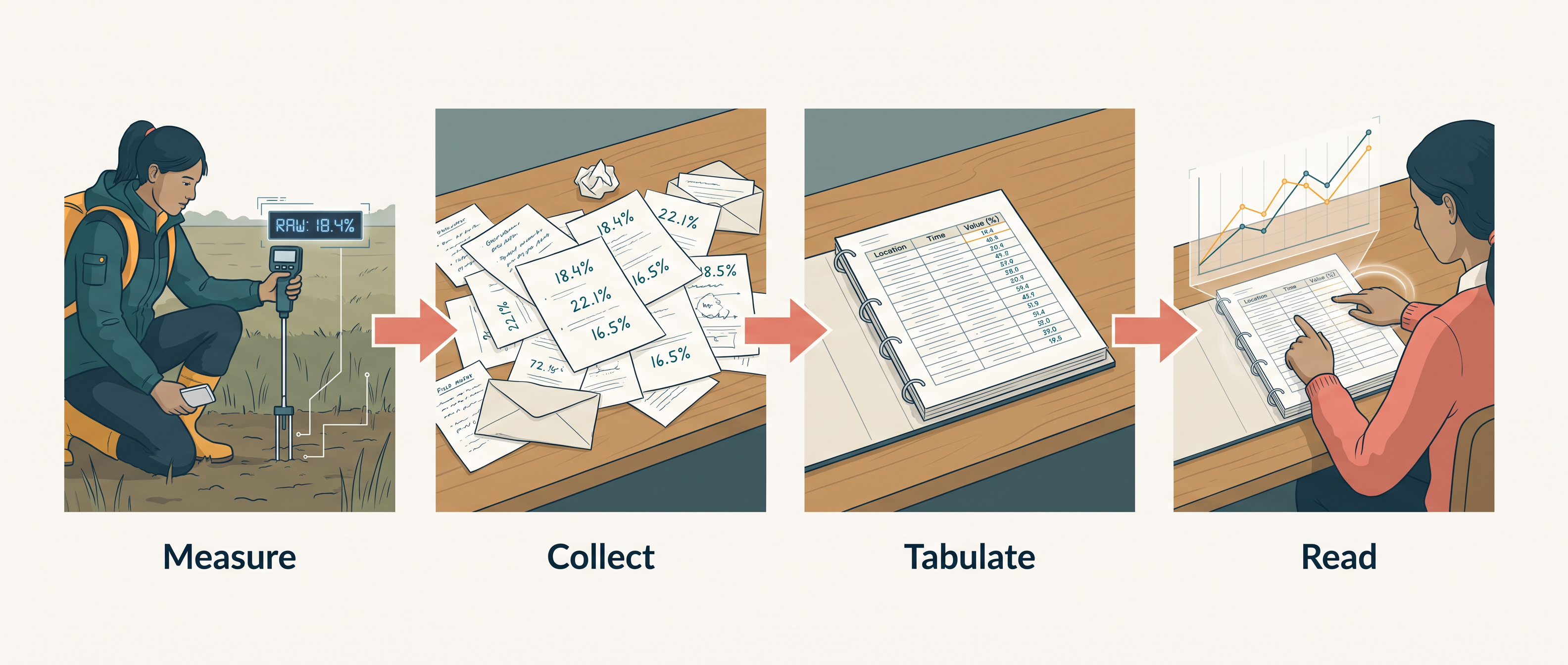
Fig. 1.0 – The journey from measurement to information.

Curiosity Corner

Q1. How can an average be perfectly correct and still lead you badly astray? Q2. When production is said to have risen to an index of 207, what does 207 actually count — and why not simply state the tonnes? Q3. Where does the population figure printed in your geography textbook really come from, and who first collected it? Q4. Handed the marks of sixty students scattered across a page, how would you turn that jumble into something you can actually read? This chapter will let you answer every one of these — and show you the methods that make the answers trustworthy.

1.1 What Is Data?

Data are the numbers we use to describe the real world. More precisely, data are numbers that stand for measurements taken from the world around us — a temperature, a rainfall total, a distance, a head-count of people. Each number pins down something that was actually observed or measured.

The smallest unit is a single reading. A datum is one measurement on its own — one temperature, one rainfall figure, one distance. Strictly, ‘data’ is the plural and ‘datum’ the single form, though in everyday use ‘data’ is often made to cover both.

Data In Everyday Life

Everyday news is full of data. You might hear that Barmer, in the dry west of Rajasthan on the edge of the Thar desert, received 20 centimetres of continuous rain, or that Banswara, in the far south of Rajasthan, recorded 35 centimetres of rain at a stretch in 24 hours. A centimetre of rain is a depth of water — imagine that depth standing over the ground before it drains or soaks away.

You might also read that the rail distance from New Delhi to Mumbai is 1385 kilometres if you travel via Kota and Vadodara, but 1542 kilometres if you go via Itarsi and Manmad. Both figures are correct; the distance simply depends on the route taken. Every one of these numbers is a datum, and together they are data.

The Problem With Raw Data

There is an enormous volume of data in the world today, and that abundance is itself a difficulty. In its raw form — a loose pile of separate readings — data rarely tells you anything on its own. Two rainfall figures side by side do not explain themselves, and a list of distances is just a list.

To reach a sound conclusion, the raw numbers have to be worked on, and that working can take several forms. The figures may be derived algorithmically, put through a fixed set of steps followed the same way every time, like a recipe. They may be deduced logically, reasoned out from what the numbers must mean when read together. Or they may be calculated statistically from many data at once — combined, averaged or compared across a whole set. Often all three happen before a number is ready to be trusted.

When Data Becomes Information

Once raw data has been worked on in this way, it turns into information. Information is a meaningful answer to a question, or a meaningful signal that sets off further questions of its own.

The difference between data and information runs through the whole chapter. Data is the raw material: individual measurements, true but mute. Information is what those measurements say once they are ordered and interpreted. That a city recorded 41 °C is a datum; that the city is living through its hottest week of the year is information. The two are not opposites — information is built out of data — but they are not the same thing, and confusing them is where careless reading begins.

1.2 Need Of Data

Maps have always been the geographer’s main tool. A map shows where things are — where the forest thins, where the rivers run, where the towns cluster. But a map struggles to show how much, and it cannot easily show change over time. That is the work data does. The spread of a phenomenon across space, and its growth from one year to the next, are set out in tables of numbers.

Why Numbers, Not Just Description

Geography studies phenomena that are tied to one another across the earth’s surface. Rainfall shapes farming, farming shapes settlement, settlement shapes traffic. These interactions are driven by many variables — quantities that change from place to place and from time to time — and such variables are explained best in quantitative terms, that is, in numbers rather than in words alone. For this reason, statistical analysis has become a necessity in modern geography.

What It Takes To Study One Question

Consider what studying the cropping pattern of an area actually demands. You would need the cropped area, the crop yield and production, the irrigated area, the amount of rainfall, and the inputs used — fertiliser, insecticides and pesticides. Description alone cannot hold all this; only measured figures can.

The growth of a city makes the same demand in a different setting. To study it you would need the total population, its density (how many people live in each unit of area), the number of migrants arriving, the occupations people follow, their salaries, the industries present, and the means of transport and communication. Each of these is a variable, and each must be measured before the city’s growth can be understood.

Two very different questions — one rural and agricultural, one urban — turn out to need the same thing: reliable data. This is why data plays so central a role in geographical analysis.

1.3 Presentation Of The Data

Collecting the right numbers is not enough. How those numbers are presented and read decides whether they help you or harm you. The oldest warning in statistics is a short story, and it is worth walking through slowly.

A traveller once measured a river before crossing it with his family, worked out a perfectly correct average, and trusted it. The reasoning was sound. The outcome was not.

Worked Case

WC 1.1 — The River And The Average The situation: A traveller, his wife and their five-year-old child had to cross a river (this chapter’s own story, told under ‘Presentation of the Data’). Before crossing, he measured the water’s depth at four points. The working: Depths at the four points were 0.6 m, 0.8 m, 0.9 m and 1.5 m. \[\text{Average depth} = \frac{0.6 + 0.8 + 0.9 + 1.5}{4} = \frac{3.8}{4} = 0.95 \text{ m}\] Here 0.95 m is the mean depth in metres. The child’s height was 1 m. Because the average depth, 0.95 m, was less than the child’s height of 1 m, the traveller judged the crossing safe and led his family in. The child drowned.

On the far bank he sat asking himself, ‘Lekha Jokha Thahe, to Bachha Dooba Kahe?’ — why did the child drown when the average depth was within everyone’s reach? The answer sits in the fourth measurement. One point was 1.5 m deep, half a metre over the child’s height, and that single deep spot was enough. This is a statistical fallacy: a conclusion that is arithmetically correct yet false to the real situation, because a summary figure such as an average hides the variation underneath it. The average of 0.95 m was true, and it was also useless — because a river is crossed point by point, not on average.

Curiosity Corner

Q1. How can an average be perfectly correct and still lead you badly astray?

A. The river’s average depth, 0.95 m, was arithmetically flawless — yet one point ran to 1.5 m, well over the child’s height. An average blends high and low into a single middle figure and so hides the extremes. A number can be exactly right and still describe a situation that existed at no single point. Always ask what the average is covering up.

Collecting Is Only Half The Work

The lesson is not that data lies. It is that data must be presented and interpreted with care. It is important to collect data to know the facts and figures, but it is equally important to present them well, because a poorly read figure can point you in exactly the wrong direction.

This is why statistical methods now matter so much. The use of statistics in analysing data, presenting it and drawing conclusions plays a significant role in almost every discipline that relies on data, and geography is firmly among them.

From Words To Numbers

Think about how phenomena are spread across the earth. The concentration of population, of forest, or of a network of transport and communication does not stay fixed — it varies over space and it changes over time. Data is what lets us describe that variation precisely rather than vaguely.

Older geography leaned on qualitative description, accounts given in words, such as saying a region is ‘thickly peopled’. Modern geography has shifted toward quantitative analysis, which attaches a measured figure to the same claim and so allows one place or one year to be compared exactly against another. This shift is why analytical tools and techniques have grown so important: they make a study more logical and let it reach a precise conclusion rather than a loose impression.

That precision is needed at every stage, not just at the end. Careful quantitative technique runs right through the work — from collecting and compiling the data, through its tabulation, organisation and ordering, to the final analysis and the conclusions drawn from it.

1.4 Sources Of Data

Geographers gather data in two broad ways, and the difference between them is simply who did the collecting. Data collected for the very first time — directly by an individual, a group, or an institution — comes from a primary source. Data that someone else has already collected, and that you take from a published or unpublished record, comes from a secondary source.

The distinction is one of first-hand against second-hand. A primary source is first-hand: you go out and measure or ask, so the data is fresh and shaped exactly to your question. A secondary source is second-hand: the data already exists, gathered by others for their own purposes, and you borrow it. Neither is better in every case — a primary survey is precise but slow and costly, while a secondary record is quick to reach but may not fit your question exactly.

The full range of methods, on both sides of this divide, is set out in Fig. 1.1. On the primary side sit personal observation, interview, questionnaire or schedule, and a group of other field methods. On the secondary side, the sources are first split into published and unpublished, and each of those into finer types.

Fig. 1.1

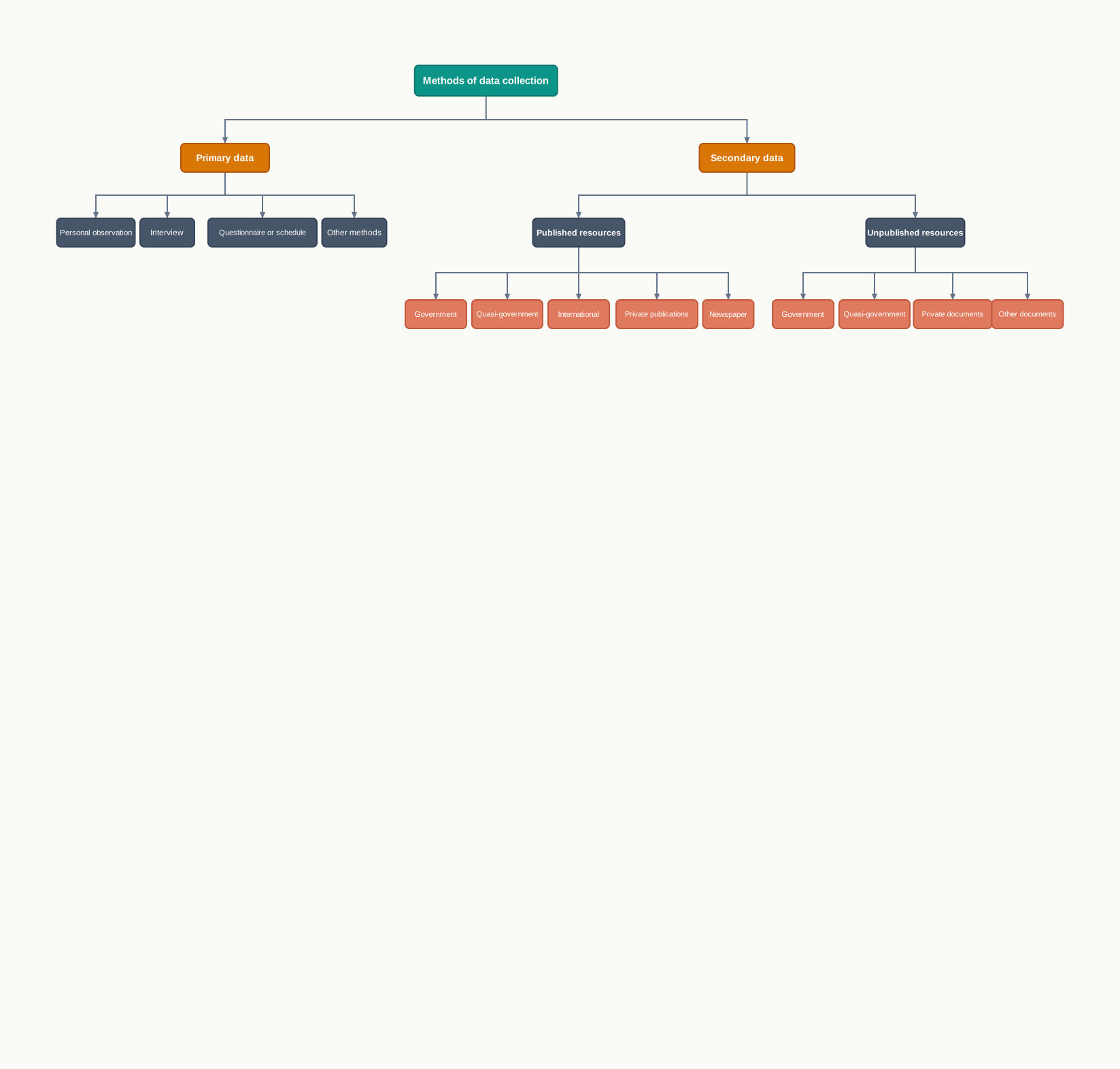
Fig. 1.1 – Primary and secondary data sources.

Read It

Fig. 1.1 Read from the top down. The single box at the top is all data collection; each step down splits it into kinds, and a branch ends at one specific type of source. Following a branch tells you which category a source belongs to. Limit: the tree names the categories but does not say which source is most reliable, or which best fits a given study.

1.5 Sources Of Primary Data

Primary data is gathered first-hand, in the field, by four main methods: personal observation, interview, questionnaire or schedule, and a set of direct-measurement techniques.

1.5.1 Personal Observations

This method collects information by watching and recording directly in the field, whether by one person or a team. In a field survey — going to a place and noting what is there for yourself — a geographer can gather a wide range of facts: the relief features (the shape of the land, its hills and valleys), the drainage patterns (how the streams and rivers are arranged), the types of soil and natural vegetation, and, on the human side, the population structure, the sex ratio (the number of females per 1000 males), the level of literacy, the means of transport and communication, and the pattern of urban and rural settlements.

Direct observation is only as good as the observer. The person carrying it out must already have theoretical knowledge of the subject, so they know what to look for, and a scientific attitude, so they record what is actually there rather than what they expect or wish to see. Without that discipline the observation is biased, and biased data is worse than none.

1.5.2 Interview

In an interview, the researcher gets information straight from a respondent — the person answering — through direct conversation. Done carelessly it yields little, so an interviewer follows a set of precautions.

Prepare first. Draw up a precise list of the items you need to ask about, and be clear in your own mind about the objective of the survey.

Put the respondent at ease. Before any sensitive question, take the person into confidence and assure them their answers will be kept secret. Create a relaxed atmosphere so they can explain the facts without hesitation. Keep the language of your questions simple and polite, so people feel motivated to answer. And never ask anything that could wound a person’s self-respect or religious feelings.

Close well. At the end, ask whether there is anything more the respondent would like to add beyond what you asked, and thank them warmly for sparing their time.

1.5.3 Questionnaire/Schedule

A questionnaire is a printed set of questions. In its simplest form, each question comes with possible answers and the respondent just tick-marks the choice that fits; in a fuller form, the questions are structured and space is left for the respondent to write an opinion. Whatever the form, the objectives of the survey should be stated clearly on it. Because it can be handed out widely, or even mailed to far-flung places, a questionnaire suits a survey spread over a large area. Its limitation is plain: only literate, educated people can fill it in, so anyone who cannot read is left out.

A schedule carries much the same questions about the matter under investigation, but it is filled in differently. With a questionnaire, respondents write their own answers; with a schedule, a trained enumerator — the fieldworker who conducts the survey — puts the questions and records the answers himself. This one difference is decisive: because the enumerator does the writing, a schedule can collect information from literate and illiterate respondents alike, which is its main advantage over the questionnaire.

1.5.4 Other Methods

Some data is taken straight from the ground by direct measurement. The properties of soil and water are measured in the field with a soil kit and a water quality kit — portable sets of tools for testing them on the spot. In the same way, field scientists judge the health of crops and vegetation using transducers, instruments that turn a physical property into a signal that can be read as a number (Fig. 1.2).

Fig. 1.2

Fig. 1.2 – Measuring crop health in the field.

1.6 Secondary Source Of Data

Secondary data is data someone has already collected and set down in a record. These records fall into two groups — published and unpublished — and between them they cover government publications, documents and reports of every kind.

1.6.1 Published Sources

Published secondary sources come in several kinds.

Government publications are among the most important. The ministries and departments of the Government of India, the state governments and the District Bulletins all publish data regularly. This is where the biggest official datasets live: the Census of India, brought out by the Office of the Registrar General of India, which counts the whole population; the reports of the National Sample Survey; the Weather Reports of the Indian Meteorological Department; the Statistical Abstracts published by state governments; and the periodical reports of various Commissions. Some of these publications are shown in Fig. 1.3.

Fig. 1.3

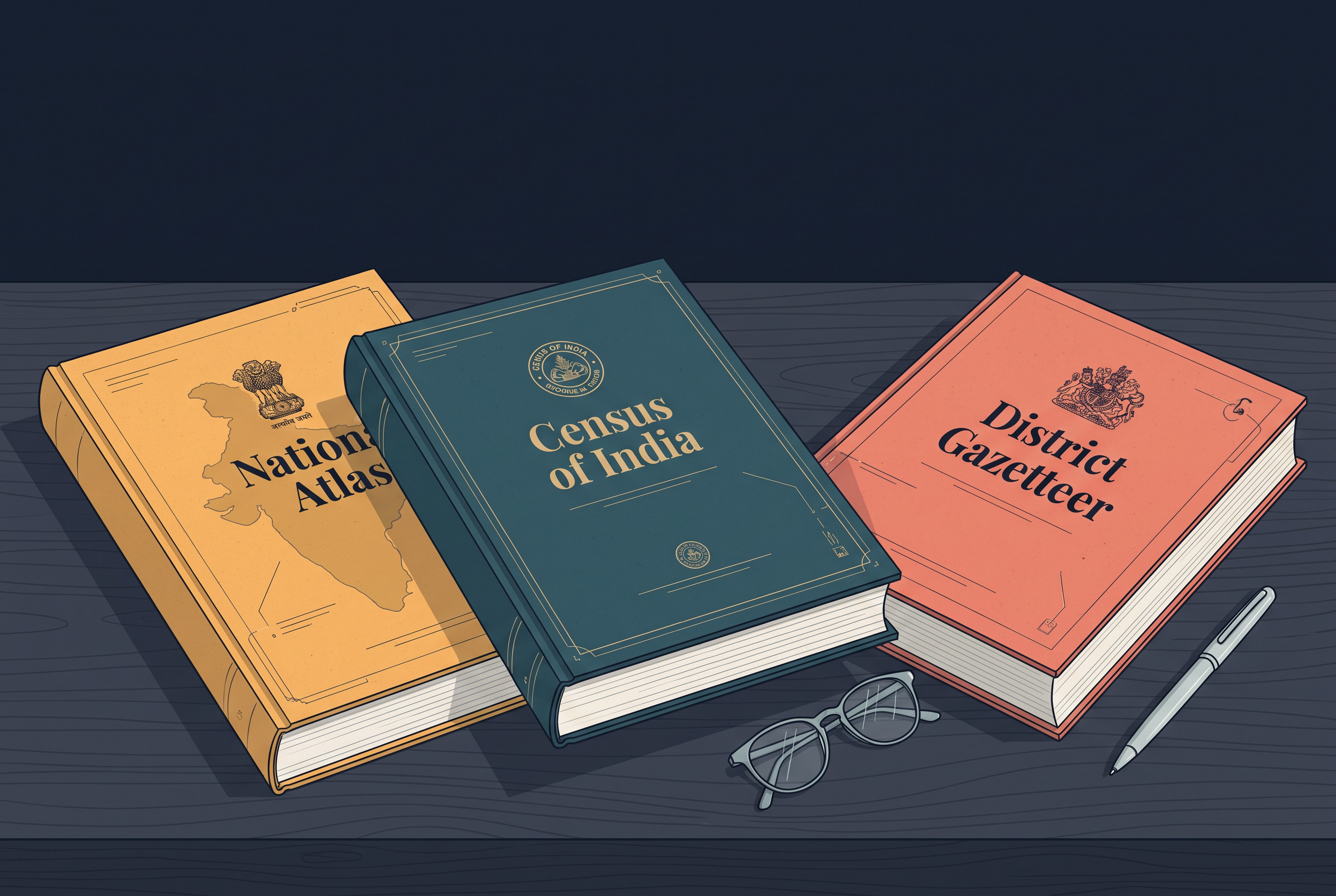
Fig. 1.3 – Government publications for secondary data.

Curiosity Corner

Q3. Where does the population figure printed in your geography textbook really come from, and who first collected it?

A. From the Census of India, published by the Office of the Registrar General of India. Government enumerators first count the population directly, house to house; the textbook then borrows their published totals. So for the textbook it is a secondary, published, government source.

Semi- or quasi-government publications come from bodies that sit alongside government: the Urban Development Authorities and Municipal Corporations of cities and towns, and the Zila Parishads, or District Councils, that govern rural districts.

International publications are the yearbooks, reports and monographs put out by agencies of the United Nations — among them UNESCO (the UN’s education, science and culture body), UNDP (its development programme), WHO (the World Health Organisation) and FAO (the Food and Agriculture Organisation). Titles that appear regularly include the Demographic Year Book, the Statistical Year Book and the Human Development Report, some of which are shown in Fig. 1.4.

Fig. 1.4

Fig. 1.4 – United Nations publications for secondary data.

Beyond these, private publications — the yearbooks, surveys, research reports and monographs of newspapers and private organisations — add to the store. So do newspapers and magazines, whether daily, weekly, fortnightly or monthly, which are among the easiest secondary sources to reach. And in recent times electronic media, above all the internet, has become a major source of secondary data.

1.6.2 Unpublished Sources

Not every record is printed for the public. A great deal of useful data sits in unpublished documents kept at different levels of governance.

Government documents are the first kind — reports, monographs and papers maintained as unpublished record. The clearest example is the village revenue record kept by the patwari, the village-level revenue official who maintains land records; his registers are an important source of information at the village scale.

Quasi-government records are the second kind: the periodical reports and development plans drawn up and held by Municipal Corporations, District Councils and Civil Services departments.

Private documents are the third: the unpublished reports and records of companies, trade unions, political and apolitical organisations, and residents’ welfare associations.

1.7 Tabulation And Classification Of Data

Data does not arrive in usable shape. Whether it comes from a primary survey or a secondary record, it first appears as a big jumble of figures that means little at a glance. This unworked mass is called raw data. Before it can yield any meaningful inference, it has to be put in order — and that ordering is done through tabulation and classification.

The simplest tool for the job is the statistical table, a systematic arrangement of data in rows and columns. A table does several things at once. It simplifies the presentation, so a reader is not lost among loose numbers. It makes comparison easy, because like is set beside like. It lets the reader find any particular figure quickly. And it packs a huge mass of data into an orderly form that takes up very little space.

In short, a table turns a heap of numbers into something a person can actually read. The sections that follow build on this: once data is tabulated, it can be classified, grouped and summarised further.

1.8 Data Compilation And Presentation

Once data has been collected and tabulated, it can be presented in three different forms: in absolute terms, as percentages or ratios, or as index numbers. The three are not rivals; each answers a different question. Absolute figures tell you the size of something. Percentages and ratios set that size against a common measure, so different things can be compared fairly. Index numbers track how a value has changed from a chosen starting point. Choosing the right form is part of presenting data honestly.

1.8.1 Absolute Data

When data is shown in its original form, as whole numbers, it is called absolute data — the same thing the last section called raw data. A total population, the total production of a crop, the output of a manufacturing industry: each is an absolute figure, a plain count of the thing itself. Table 1.1 sets out the absolute population of India and of some selected states and Union Territories from the 2011 Census.

Table

Table 1.1 Caption: Population of India and selected states/Union Territories, 2011 — the total population, then split into persons, males and females. | State/UT Code | India/State/Union Territory | Persons | Males | Females | |—|—|—|—|—| | 1 | 2 | 3 | 4 | 5 | | | INDIA¹ | 1,21,05,69,573 | 62,31,21,843 | 58,74,47,730 | | 1. | Jammu and Kashmir² | 1,25,41,302 | 66,40,662 | 59,00,640 | | 2. | Himachal Pradesh | 68,64,602 | 34,81,873 | 33,82,729 | | 3. | Punjab | 2,77,43,338 | 1,46,39,465 | 1,31,03,873 | | 4. | Chandigarh³ | 10,55,450 | 5,80,663 | 4,74,787 | | 5. | Uttarakhand | 1,00,86,292 | 51,37,773 | 49,48,519 | | 6. | Haryana | 2,53,51,462 | 1,34,94,734 | 1,18,56,728 | | 7. | National Capital Territory of Delhi | 1,67,87,941 | 89,87,326 | 78,00,615 | | 8. | Rajasthan | 6,85,48,437 | 3,55,50,997 | 3,29,97,440 | | 9. | Uttar Pradesh | 19,98,12,341 | 10,44,80,510 | 9,53,31,831 | | 10. | Bihar | 10,40,99,452 | 5,42,78,157 | 4,98,21,295 |

¹ inclusive of all territorial boundary of India ² excluding PoK ³ Union Territory Source: Census, 2011

Notice the small superscript numbers beside some names; they point to footnotes below the table. Footnotes are useful because they let a table stay clean while still carrying the fine print — here, that India’s figure covers its full territorial extent, that the Jammu and Kashmir count excludes Pakistan-occupied Kashmir, and that Chandigarh is a Union Territory rather than a state. Without footnotes, either the table would be cluttered with explanations or these qualifications would be lost.

Read It

Table 1.1 The three right-hand columns give the total population, then that same total split into males and females; the superscripts point to footnotes flagging exceptions. India’s row holds the largest count, and among the states listed Uttar Pradesh is the biggest. Limit: an absolute count tells you how many people live somewhere, not how crowded they are — a large number may still be thinly spread over a wide area.

1.8.2 Percentage/Ratio

Sometimes data is more useful as a ratio or a percentage than as a raw count. Such figures are worked out from a common parameter — a shared base that makes comparison fair. The literacy rate, the growth rate of population, and the share of agricultural or industrial products in a total are all of this kind. Table 1.2 shows India’s literacy rate, decade by decade, from 1951 to 2011.

Table

Table 1.2 Caption: Literacy rate of India, 1951 to 2011, in per cent, for persons, males and females. | Year | Person | Male | Female | |—|—|—|—| | 1951 | 18.33 | 27.16 | 8.86 | | 1961 | 28.3 | 40.4 | 15.35 | | 1971 | 34.45 | 45.96 | 21.97 | | 1981 | 43.57 | 56.38 | 29.76 | | 1991 | 52.21 | 64.13 | 39.29 | | 2001 | 64.84 | 75.85 | 54.16 | | 2011 | 73.0 | 80.9 | 64.6 |

Source: Census, 2011

The literacy rate is the percentage of people who can read and write, and it is found with a simple formula:

\[\text{Literacy rate} = \frac{\text{Total literates}}{\text{Total population}} \times 100\]

Here ‘total literates’ is the number of people able to read and write, ‘total population’ is everyone counted, and the answer comes out as a percentage. Expressing literacy this way lets you compare a small state with a large one fairly, because a percentage does not depend on the size of the population behind it.

Read It

Table 1.2 Each row is a Census decade; the columns give the literacy rate — the share of people who can read and write — for all persons, then males and females separately. Read down and the figures rise every decade, while the male–female gap slowly narrows. Limit: this is the all-India figure, so it hides how literacy differs between states, and between rural and urban areas.

1.8.3 Index Number

An index number is a statistical measure built to show how a variable, or a group of related variables, has changed — over time, between places, or across other characteristics. Index numbers do two jobs: they track change over a period, and they let you compare economic conditions across different locations, industries, cities or countries. They are used widely in economics and business to follow movements in price and quantity.

There are several ways to work out an index number, but the most common is the simple aggregate method:

\[\text{Index number} = \frac{\sum q_1}{\sum q_0} \times 100\]

Here \(\sum q_1\) is the total production in the current year, and \(\sum q_0\) is the total production in the base year — the year chosen as the starting point for comparison. The base year’s value is set at 100, and every other year is measured against it. Table 1.3 does exactly this for the production of iron ore in India, taking 1970-71 as the base year.

Table

Table 1.3 Caption: Production of iron ore in India, and its index number, 1970-71 to 2000-01, with 1970-71 as the base year. | Year | Production (in million tonnes) | Calculation | Index Number | |—|—|—|—| | 1970-71 | 32.5 | (32.5 ÷ 32.5) × 100 | 100 | | 1980-81 | 42.2 | (42.2 ÷ 32.5) × 100 | 130 | | 1990-91 | 53.7 | (53.7 ÷ 32.5) × 100 | 165 | | 2000-01 | 67.4 | (67.4 ÷ 32.5) × 100 | 207 |

Source: India: Economic Year Book, 2005

The working is the same for every row. Take the year’s production, divide it by the base year’s production, and multiply by 100. For 1980-81, that is 42.2 ÷ 32.5 × 100, which the table rounds to an index of 130. Because 1970-71 is fixed at 100, each later index shows that year’s output as a share of the base year’s — so 130 means output was about 30 per cent higher than in 1970-71.

Curiosity Corner

Q2. When production is said to have risen to an index of 207, what does 207 actually count — and why not simply state the tonnes?

A. The base year, 1970-71, is fixed at 100. An index of 207 means production had reached 207 per cent of that base — just over double. It counts no tonnes directly; it shows change relative to the start, which makes the trend easy to compare across years.

By 2000-01 the index had reached 207, meaning iron-ore production had grown to a little over twice its 1970-71 level. The strength of an index number is exactly this: it turns a set of awkward, differently sized figures into a clear story of rise or fall, all measured from the same starting line.

1.9 Processing Of Data

Processing raw data means putting it through tabulation and classification — sorting it into selected classes so that its meaning can surface. Table 1.4 gives a good example to work with: the scores of 60 students in a geography paper.

Table

Table 1.4 Caption: Score of 60 students in a geography paper. | | | | | | | | | | | |—|—|—|—|—|—|—|—|—|—| | 47 | 02 | 39 | 64 | 22 | 46 | 28 | 02 | 09 | 10 | | 89 | 96 | 74 | 06 | 26 | 15 | 92 | 84 | 84 | 90 | | 32 | 22 | 53 | 62 | 73 | 57 | 37 | 44 | 67 | 50 | | 18 | 51 | 36 | 58 | 28 | 65 | 63 | 59 | 75 | 70 | | 56 | 58 | 43 | 74 | 64 | 12 | 35 | 42 | 68 | 80 | | 64 | 37 | 17 | 31 | 41 | 71 | 56 | 83 | 59 | 90 |

As printed, this data is ungrouped — the sixty scores are simply listed one after another, in no particular order. You can read off any single student’s mark, but you cannot see the shape of the whole: how many did well, how many struggled, where most of the class sat. Sixty loose numbers are still a jumble.

The first step in processing, therefore, is to group the data. Grouping reduces its volume — sixty separate figures become a handful of classes — and makes the pattern easy to see. The next sections show exactly how this grouping is done.

Read It

Table 1.4 Each of the sixty cells is one student’s score, ranging from 02 to 96. Reading across the rows gives you individual marks, one by one. Limit: in this raw, ungrouped form the table shows every value but no pattern — you cannot tell how many students scored high or low until the scores are grouped into classes.

1.10 Grouping Of Data

To group raw data you must decide two things: how many classes to make, and how wide each class should be. That width is the class interval, and each class is a band the data falls into. Both choices follow from the range of the data — the distance between its smallest and largest values.

The scores in Table 1.4 run from 02 to 96. A convenient choice, then, is ten classes each ten units wide: 0-10, 10-20, 20-30, and so on up to 90-100. Ten bands of ten cover the whole stretch from 0 to 100 neatly, and each band is small enough to show the pattern without leaving many classes empty. The result is set out in Table 1.5.

Table

Table 1.5 Caption: Grouping the scores into classes and marking tallies to obtain the frequency of each class. | Group | Numerical of Raw Data | Tally Marks | Number of Individual | |—|—|—|—| | 0-10 | 02,02,09,06 | IIII | 4 | | 10-20 | 10,15,18,12,17 | IIIII | 5 | | 20-30 | 22,28,26,22,28 | IIIII | 5 | | 30-40 | 39,32,37,36,35,37,31 | IIIII II | 7 | | 40-50 | 47,46,44,43,42,41 | IIIII I | 6 | | 50-60 | 53,57,50,51,58,59,56,58,56,59 | IIIII IIIII | 10 | | 60-70 | 64,62,67,65,63,64,68,64 | IIIII III | 8 | | 70-80 | 74,73,75,70,74,71 | IIIII I | 6 | | 80-90 | 89,84,84,80,83 | IIIII | 5 | | 90-100 | 96,92,90,90 | IIII | 4 | | | | | Σf = N = 60 |

(In the Tally Marks column, each bundle of five strokes stands for one completed group in the Four and Cross Method, explained in the next section.)

The third column, the tally marks, records each score with a stroke as it is sorted into its class; the fourth column simply counts those strokes. How the tallying is actually carried out is the subject of the next section.

1.11 Process Of Classification

With the number of classes and the class interval fixed, the raw data can be sorted into those classes. This is done by the Four and Cross Method, also called tallying. You take each value in turn and put one stroke in the class it belongs to. The very first score in Table 1.4 is 47; since 47 falls in the 40-50 class, a single tally mark goes against 40-50 in column three of Table 1.5. Work through all sixty scores this way and every one lands in its class. The strokes are drawn in bundles of five — four upright, the fifth struck across them — which is what the name refers to, and counting in fives makes the totals quick to read.

1.11.1 Frequency Distribution

Once the raw data is grouped class by class, the number of individuals in each class is called its frequency. The whole arrangement — each class set against the count that falls in it — is a frequency distribution, and it shows how the values of a variable are spread across the classes. Table 1.6 lays out the frequency distribution for the sixty scores.

Table

Table 1.6 Caption: Frequency distribution of the sixty scores by the exclusive method, with simple frequency (f) and cumulative frequency (Cf). | Group | f | Cf | |—|—|—| | 00-10 | 4 | 4 | | 10-20 | 5 | 9 | | 20-30 | 5 | 14 | | 30-40 | 7 | 21 | | 40-50 | 6 | 27 | | 50-60 | 10 | 37 | | 60-70 | 8 | 45 | | 70-80 | 6 | 51 | | 80-90 | 5 | 56 | | 90-100 | 4 | 60 | | | Σf = N = 60 | |

At a glance the distribution now tells a story the raw list could not. Most students cluster in the middle classes, and the single largest group — ten of them — scored between 50 and 60; the tails, at the very lowest and highest classes, are thin. Sixty scattered numbers have become a readable shape.

Curiosity Corner

Q4. Handed the marks of sixty students scattered across a page, how would you turn that jumble into something you can actually read?

A. Group the marks into classes — here, ten bands of ten — then tally each mark into its class and count the tallies. The result is a frequency distribution: a short table showing how many students fall in each band, so the shape of the whole class appears at once.

Frequencies come in two kinds, simple and cumulative.

1.11.2 Simple Frequencies

A simple frequency, written ‘f’, is just the number of individuals falling in one class (Table 1.6). Add up the simple frequencies of all the classes and you get the total number of observations in the whole series. In statistics this total is written as N, and it equals the sum of all the frequencies:

\[\sum f = N = 60\]

Here \(\sum f\) means ‘the sum of all the frequencies’, and for our data it comes to 60 — exactly the number of students we started with, which is the check that nothing has been lost or double-counted.

1.11.3 Cumulative Frequencies

A cumulative frequency, written ‘Cf’, is built by adding each class’s simple frequency to the running total so far, as the third column of Table 1.6 does. The first simple frequency is 4, so the first cumulative frequency is 4. The next simple frequency, 5, is added to give 9. Carry on adding down the column and the last cumulative frequency comes to 60 — again equal to N, or \(\sum f\).

The value of a cumulative frequency is that it answers ‘how many below this point’ at a glance. From Table 1.6 you can read straight off that 27 individuals scored less than 50, and that 45 of the 60 lie below a score of 70.

Each simple frequency belongs to a class, and there are two ways of setting up those classes — the exclusive method and the inclusive method.

1.11.4 Exclusive Method

In the exclusive method, shown in Table 1.6, each class is written with two numbers, and the upper number of one class is the same as the lower number of the next. The upper limit of 20-30, for instance, is 30, which is also the lower limit of 30-40, so 30 appears in both. The rule is that a value equal to 30 is placed in the class where 30 is the lower limit (30-40) and kept out of the class where it is the upper limit (20-30). Because each class excludes its own upper limit, the method is called exclusive.

Read this way, the classes mean ‘0 and under 10’, ‘10 and under 20’, ‘20 and under 30’, and so on up to ‘90 and under 100’. Each class still spans ten units: the 20-30 class, for example, holds 20, 21, 22, 23, 24, 25, 26, 27, 28 and 29.

1.11.5 Inclusive Method

In the inclusive method, shown in Table 1.7, a value equal to the upper limit of a class is included in that same class. The classes are written differently — 0-9, 10-19, 20-29, and so on — so that the upper limit of one class differs by 1 from the lower limit of the next, and no number is shared between two classes.

Table

Table 1.7 Caption: The same frequency distribution set out by the inclusive method. | Group | f | Cf | |—|—|—| | 0-9 | 4 | 4 | | 10-19 | 5 | 9 | | 20-29 | 5 | 14 | | 30-39 | 7 | 21 | | 40-49 | 6 | 27 | | 50-59 | 10 | 37 | | 60-69 | 8 | 45 | | 70-79 | 6 | 51 | | 80-89 | 5 | 56 | | 90-99 | 4 | 60 | | | Σf = N = 60 | |

Each class still spreads over ten units. The 50-59 class, for instance, takes in all ten values from 50 to 59: 50, 51, 52, 53, 54, 55, 56, 57, 58 and 59. Both the lower and the upper limit belong to the class, which is why the method is called inclusive.

The two methods sort the same data into the same counts — compare the frequencies in Tables 1.6 and 1.7 and they match class for class. They differ only in how a boundary value is handled: the exclusive method pushes it up to the next class, while the inclusive method keeps the limits apart so the question never arises.

1.11.6 Frequency Polygon

A graph of a frequency distribution is called a frequency polygon. Its use is to compare two or more frequency distributions at once. In Fig. 1.5 the frequencies are shown two ways together — as a bar diagram and as a line — so that the two can be read against each other.

Fig. 1.5

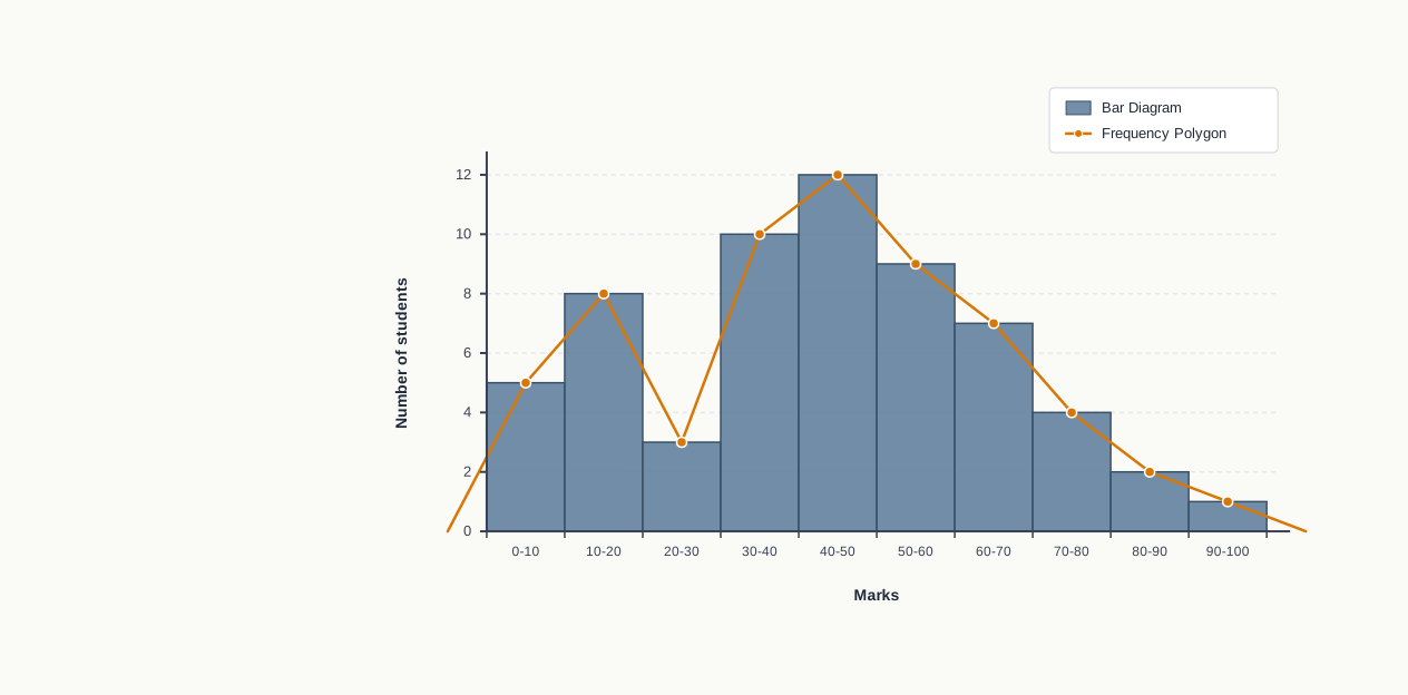
Fig. 1.5 – Bar diagram and frequency polygon of student scores.

1.11.7 Ogive

When frequencies are added into cumulative frequencies and listed in a cumulative frequency table, the curve you get by plotting those cumulative frequencies is called an ogive (pronounced ‘ojive’). It can be drawn in either of two ways.

The less than method starts from the upper limit of each class and goes on adding the frequencies. Plotted, these give a rising curve, as in Table 1.8 and Fig. 1.6.

Table

Table 1.8 Caption: Cumulative frequency by the less than method. | Less than Method | Cf | |—|—| | Less than 10 | 4 | | Less than 20 | 9 | | Less than 30 | 14 | | Less than 40 | 21 | | Less than 50 | 27 | | Less than 60 | 37 | | Less than 70 | 45 | | Less than 80 | 51 | | Less than 90 | 56 | | Less than 100 | 60 |

Fig. 1.6

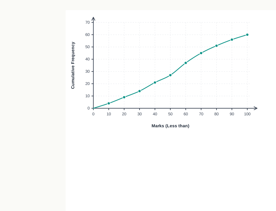
Fig. 1.6 – The less-than cumulative frequency ogive.

The more than method starts from the lower limit of each class and, working from the total cumulative frequency, subtracts each class’s frequency in turn. Plotted, these give a falling curve, as in Table 1.9 and Fig. 1.7.

Table

Table 1.9 Caption: Cumulative frequency by the more than method. | More than Method | Cf | |—|—| | More than 0 | 60 | | More than 10 | 56 | | More than 20 | 51 | | More than 30 | 44 | | More than 40 | 38 | | More than 50 | 28 | | More than 60 | 20 | | More than 70 | 14 | | More than 80 | 9 | | More than 90 | 4 |

Fig. 1.7

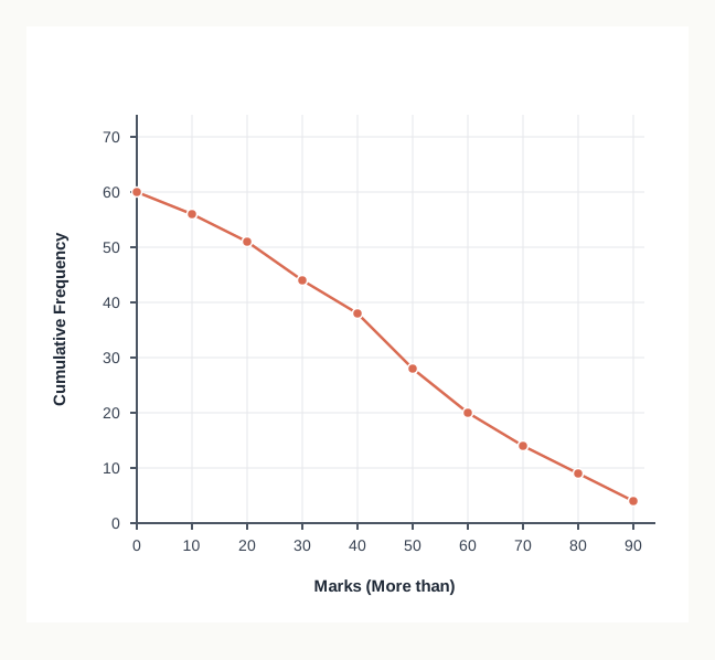
Fig. 1.7 – The more-than cumulative frequency ogive.

The two ogives can be plotted together to give a comparative picture — the less-than and more-than curves on one pair of axes — as set out in Table 1.10 and Fig. 1.8.

Table

Table 1.10 Caption: Less-than and more-than cumulative frequencies plotted together. | Marks obtained | Less than | More than | |—|—|—| | 0-10 | 4 | 60 | | 10-20 | 9 | 56 | | 20-30 | 14 | 51 | | 30-40 | 21 | 44 | | 40-50 | 27 | 38 | | 50-60 | 37 | 28 | | 60-70 | 45 | 20 | | 70-80 | 51 | 14 | | 80-90 | 56 | 9 | | 90-100 | 60 | 4 |

Fig. 1.8

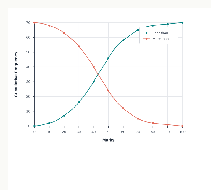
Fig. 1.8 – Less-than and more-than ogives plotted together.

Read It

Fig. 1.8 The rising curve is the less-than ogive, the falling curve the more-than ogive; the x-axis is marks and the y-axis the cumulative number of students. Reading up from any mark to a curve tells you how many students fall below it or above it. Limit: an ogive shows running totals only — it tells you how many lie beyond a mark, never any individual student’s actual score.

1.12 Summary

Data are numbers that record measurements of the real world; a single measurement is a datum, and data turns into information once it is worked on to answer a question.
Geography needs data because its phenomena, and the interactions between them, are explained best in quantitative terms rather than by description alone.
Collecting data is only half the task; how it is presented decides whether it informs or misleads — a perfectly correct average can still deceive, which is the statistical fallacy.
Data comes either from primary sources, collected first-hand (personal observation, interview, questionnaire or schedule, and other field methods), or from secondary sources, taken from published or unpublished records.
Raw data is an unusable jumble until it is tabulated and classified; the statistical table is the simplest tool for ordering it.
Data can be presented in absolute terms as raw counts, as percentages or ratios computed from a common parameter such as the literacy rate, or as index numbers that measure change against a base year set at 100.
To process a mass of readings, they are grouped into classes whose number and width follow from the range of the data.
Each value is sorted into its class by the Four and Cross Method of tallying; the count in a class is its frequency, and the whole arrangement is a frequency distribution.
A simple frequency (f) counts a single class, while a cumulative frequency (Cf) is the running total down the classes; both add up to N.
Classes may be formed by the exclusive method, which excludes each class’s upper limit, or the inclusive method, which includes both limits — and both yield the same counts.
A frequency distribution can be drawn as a frequency polygon, or as an ogive constructed by the less than method or the more than method.

Fig. 1.9

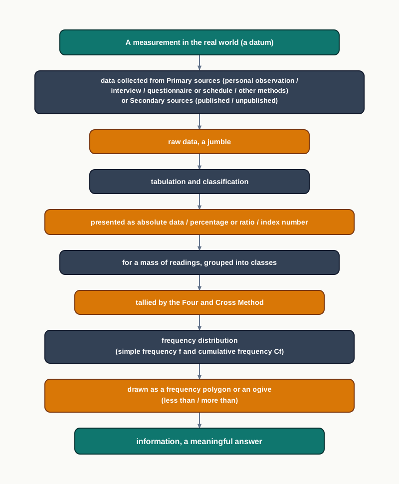
Fig. 1.9 – From a single measurement to meaningful information.

What This Chapter Cannot Tell You

The methods here arrange and present data, but they cannot judge whether the data was well collected in the first place — a biased survey still produces a tidy, and false, table. An average, a percentage or an index can be computed flawlessly and still mislead, as the river parable warned; ordering numbers does not guarantee they are the right numbers. And a grouped frequency table shows the shape of a distribution while hiding the individual values inside each class — grouping always trades detail for pattern.

1.13 NCERT Questions

A number or character which represents measurement is called:

Digit (b) Data (c) Number (d) Character

A single datum is a single measurement from the:

Table (b) Frequency (c) Real world (d) Information

In a tally mark grouping by four and crossing fifth is called:

Four and Cross Method (b) Tally Marking Method (c) Frequency plotting Method (d) Inclusive Method

An Ogive is a method in which:

Simple frequency is measured (b) Cumulative frequency is measured (c) Simple frequency is plotted (d) Cumulative frequency is plotted

If both ends of a group are taken in frequency grouping, it is called:

Exclusive Method (b) Inclusive Method (c) Marking Method (d) Statistical Method

Differentiate between data and information. (in about 30 words)
What do you mean by data processing? (in about 30 words)
What is the advantage of foot note in a table? (in about 30 words)
What do you mean by primary sources of data? (in about 30 words)
Enumerate five sources of secondary data. (in about 30 words)
Discuss the national and international agencies where from secondary data may be collected. (in about 125 words)
What is the importance of an index number? Taking an example examine the process of calculating an index number and show the changes. (in about 125 words)
In a class of 35 students of Geography, the following marks were obtained out of 10 marks in a unit test — 1, 0, 2, 3, 4, 5, 6, 7, 2, 3, 4, 0, 2, 5, 8, 4, 5, 3, 6, 3, 2, 7, 6, 5, 4, 3, 7, 8, 9, 7, 9, 4, 5, 4, 3. Represent the data in the form of a group frequency distribution.

1.14 Check Your Concepts

List, in order, the steps that turn the ungrouped scores of Table 1.4 into the frequency distribution of Table 1.6.
Explain how a schedule differs from a questionnaire, and why a schedule can collect information from illiterate respondents while a questionnaire cannot.
Using Table 1.2, calculate by how many percentage points female literacy rose between 1951 and 2011.
From Table 1.6, how many of the 60 students scored less than 60, and which column gives you the answer directly?
The exclusive method writes classes as 20-30, 30-40 and so on, so the number 30 appears in two classes. State the rule that decides which class 30 joins, and explain how the inclusive method avoids the ambiguity altogether.
The less-than ogive (Fig. 1.6) rises while the more-than ogive (Fig. 1.7) falls. Explain, in terms of how each is built from the cumulative frequencies, why one curve rises and the other falls.
A grouped frequency table such as Table 1.6 makes the shape of the class’s scores clear. State one thing it can no longer tell you that the raw list in Table 1.4 could.