Chapter 2: Data Processing
The morning the survey team reached the hamlet, the list of names ran longer than anyone expected. A college volunteer, sent to help, was handed one task that sounded simple: write down the age of every person in the settlement, then report the age of a ‘typical’ resident.
By noon she had a long column of numbers — toddlers, schoolchildren, farmers, and a few very old men and women who had lived in the same houses for eighty years and more. Her supervisor asked for a single figure. She added every age and divided by the number of people, the way she had been taught, and read out the result.
It did not match anyone. The number sat above almost every working adult in the hamlet, dragged upward by that handful of very elderly residents at the top of the list. Standing in a courtyard full of young families, she was holding a ‘typical age’ that described nobody in the room.
So she tried again. She lined the ages up in order and found the person exactly in the middle. Then she looked for the age that came up most often. Three methods, three different answers — and the gap between them, she began to see, was telling her something about the shape of the hamlet itself.
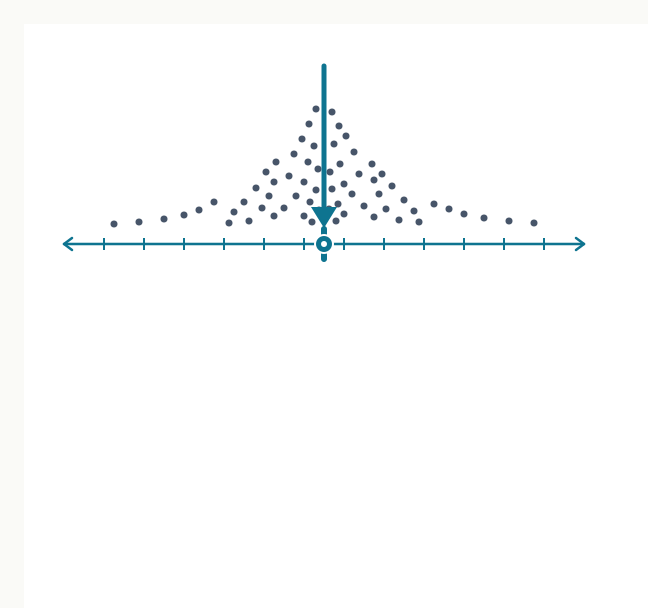
Fig. 2.0 – Concept of central tendency.
2.1 Measures Of Central Tendency
In the previous chapter you saw that organising and presenting data makes them easier to read. Tidy tables and clear graphs are only the start, though. Once the data are in order, the real work is to analyse them — to pull out what they are actually telling us.
Geographers do this with three broad families of statistical technique, shown in Fig. 2.1. The first, measures of central tendency, find the single value that best represents a whole set of observations. The second, measures of dispersion, look instead at how spread out the readings are — how far they vary, usually around that central value. The third, measures of relationship, measure how strongly two phenomena move together, such as rainfall and the incidence of flood, or fertiliser use and the yield of crops.
This chapter takes up only the first of the three. The other two build on it, so it is the right place to begin.
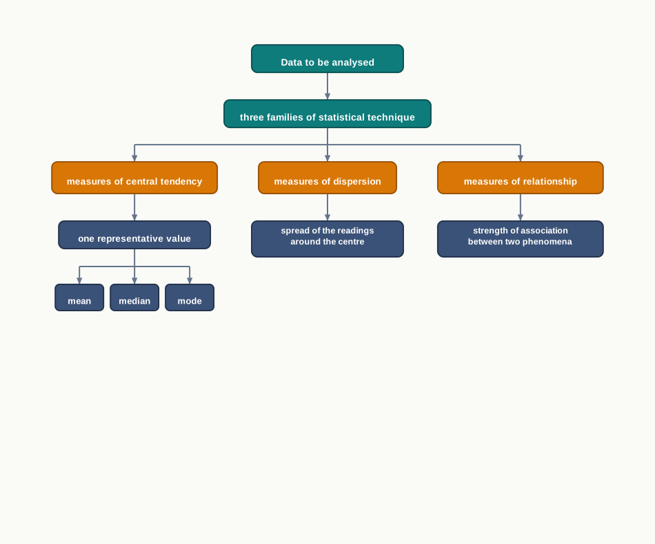
Fig. 2.1 – Families of statistical technique and central tendency measures.
Finding The Centre Of A Distribution
The characteristics a geographer measures — rainfall, elevation, density of population, levels of educational attainment, age groups — all vary from place to place and person to person. Faced with a long list of such readings, how do we sum them up in a way anyone can grasp? We look for one number that best stands for all of them.
That representative number usually lies near the centre of the distribution, not out at either extreme. The techniques that locate this centre are the measures of central tendency, and the value they return is the point about which the readings tend to cluster.
Because they stand in for a whole set, these measures are also called statistical averages. There are three of them — the mean, the median and the mode — and each finds the centre in a different way.
2.1.1 Mean
The mean is the everyday average. You add up all the values in a set and divide by how many values there are. If seven rainfall readings are totalled and that total is shared equally among the seven, the figure you get is their mean. The mean uses every value in the set — which is its great strength, and, as a later section shows, sometimes its weakness.
2.1.2 Median
The median is the value that sits exactly in the middle once the readings are placed in order. Its defining job is to split the ranked series into two equal halves, with as many readings above it as below it.
The median depends on position, not on size: it is independent of the actual values in the set. To find it, arrange the data in ascending or descending order and read off the middle-ranked value. When there is an even number of readings, and so no single value in the middle, the median is the average of the two middle-ranked values.
2.1.3 Mode
The mode is the value that occurs most often — the reading with the highest frequency in the set. Where the mean is calculated and the median is located by rank, the mode is simply spotted: it is the most common measurement.
Each of the three, then, is a different way of squeezing a data set down to a single representative number, and each suits a different kind of data. The rest of the chapter takes them one at a time.
2.2 Mean
The mean is the simple arithmetic average of the values of a variable. It is the measure most people already have in mind when they say ‘average’, and it is the one that uses every reading in the set.
How you calculate it depends on the form the data take. Ungrouped data — a plain list of readings — and grouped data — readings already sorted into classes — need different methods. And within each of those, the mean can be found by a direct method or an indirect one, as Fig. 2.2 sets out. The two methods always give the same answer; the indirect one just keeps the arithmetic smaller.
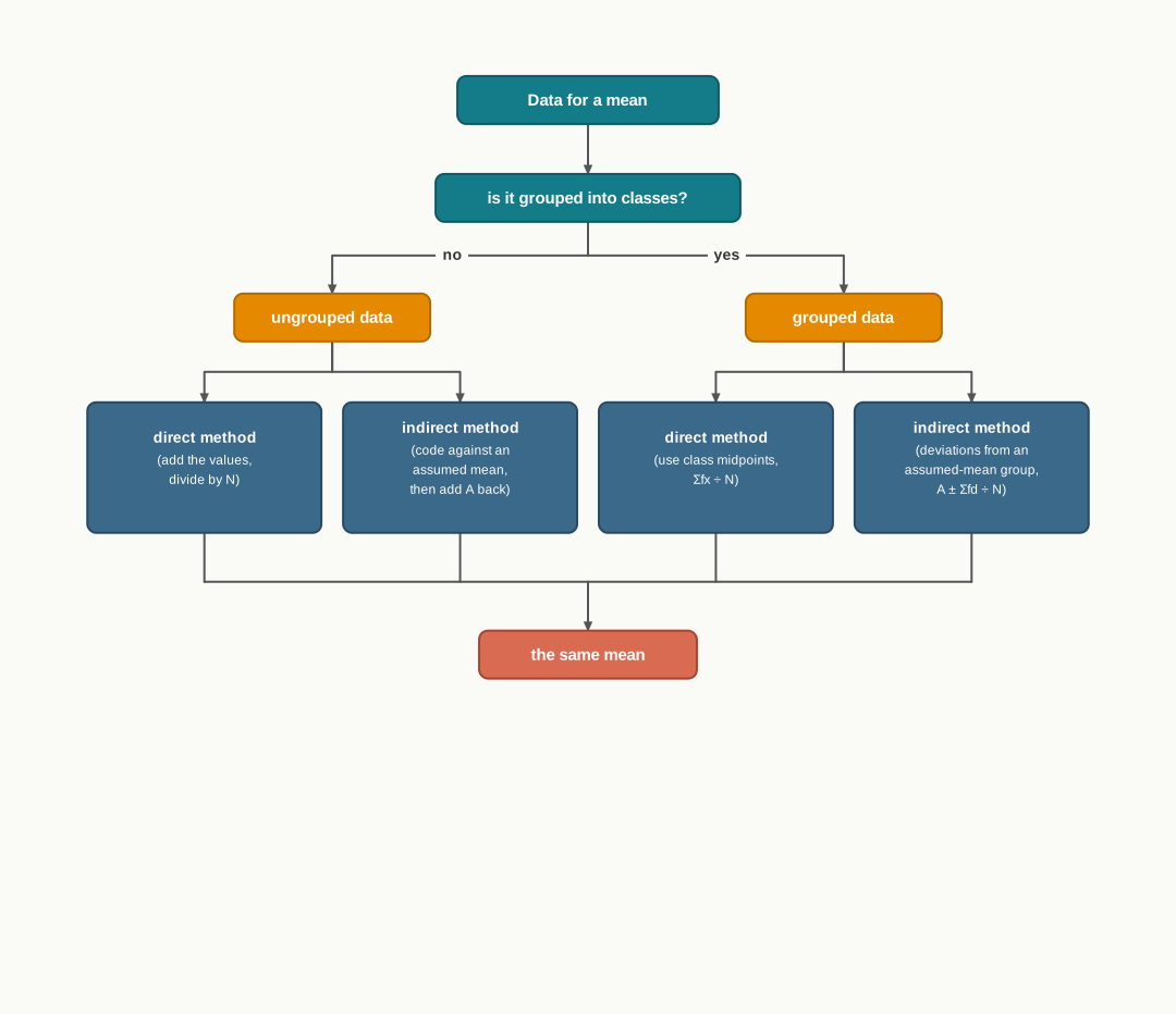
Fig. 2.2 – Routes to calculating the mean.
2.2.1 Computing Mean From Ungrouped Data
Ungrouped data are just a list: one value for each observation, none of them bundled together. Both methods below are worked on the same set of figures so you can see they agree.
2.2.1.1 Direct Method
In the direct method you add up the values of every observation and divide that total by the number of observations. Nothing is coded or adjusted first. The mean is:
\[\bar{X} = \frac{\sum x}{N}\]
Here \(\bar{X}\) is the mean; \(\sum\) (the Greek capital sigma) means ‘the sum of’; \(x\) is a single raw reading in the series; \(\sum x\) is the sum of all the readings; and \(N\) is the number of readings.
Worked Case 2.1 works this out for the normal rainfall of seven districts of the Malwa Plateau, in western Madhya Pradesh. The rainfall figures, in millimetres, are in the second column of Table 2.1; the third column belongs to the indirect method and is used later.
The mean rainfall of the plateau is 926.29 mm. Notice that no single district actually records this figure — it sits between Mandsaur’s 825 mm and Dewas’s 1083 mm, near the middle of the spread. That is what a mean is: one number that stands in for the whole region, useful for a planner who needs a single rainfall figure, but a figure that hides how much drier the west of the plateau is than the east.
2.2.1.2 Indirect Method
When there are many observations, or the numbers are large, the indirect method saves effort. It shrinks the readings to smaller numbers first. You choose an assumed mean — a round constant somewhere inside the range of the data — and subtract it from every reading. This subtraction is called coding, and the small numbers it produces are the coded scores.
For the Malwa data the rainfall lies between 800 and about 1100 mm, so 800 is taken as the assumed mean. Subtracting 800 from each reading gives the third column of Table 2.1 — deviations like 179 and 283 instead of 979 and 1083. The mean is then:
\[\bar{X} = A + \frac{\sum d}{N}\]
where \(A\) is the subtracted constant, the assumed mean; \(\sum d\) is the sum of the coded scores; and \(N\) is the number of observations.
The answer is 926.29 mm again — exactly the direct-method result. That is the point of the exercise: the two methods must agree. Coding did not change the mean; it only replaced three-digit rainfall figures with two-digit deviations, which are quicker to add and easier to add correctly. The choice of 800 was free — any constant would return the same mean, because whatever you subtract, the formula gives back.
2.2.2 Computing Mean From Grouped Data
Grouped data come already sorted into a frequency distribution — the readings are bundled into class intervals such as 50–70 or 70–90, and all we are told is how many readings fall in each class. That count is the frequency of the class. The mean can still be found by a direct or an indirect method, but with one change forced on us first.
2.2.2.1 Direct Method
When readings are grouped, the individual values lose their identity — we no longer know each worker’s exact wage, only the class it fell in. So each class is represented by its midpoint, the value halfway across the interval (the midpoint of 50–70 is 60). We treat every reading in a class as if it sat at that midpoint.
Each midpoint \(x\) is multiplied by its frequency \(f\) to give \(fx\), the whole class’s contribution. Adding these gives \(\sum fx\), which is divided by the total number of readings:
\[\bar{X} = \frac{\sum fx}{N}\]
where \(f\) is the frequency of a class, \(x\) its midpoint, and \(N\) the total number of observations, also written \(\sum f\).
Worked Case 2.3 applies this to the daily wages of factory workers. The raw distribution — five wage classes in rupees per day and the number of workers in each — is Table 2.2, and Table 2.3 carries out the full computation.
The average daily wage works out to 102.6 rupees. Because the exact wages were lost when the workers were grouped, this figure rests on an assumption: that a worker in the 90–110 class earns about 100. The mean represents the workforce as a whole, but it describes no individual worker, and it would shift if the class intervals had been drawn differently.
2.2.2.2 Indirect Method
The indirect method for grouped data follows the same idea as for ungrouped data: pick an assumed mean to shrink the arithmetic. Here the assumed mean is a whole class, chosen near the middle of the series because that keeps the deviations small. For the wage data the assumed-mean group is 90–110, whose midpoint is 100, so \(A = 100\). The formula is:
\[\bar{X} = A \pm \frac{\sum fd}{N}\]
where \(A\) is the midpoint of the assumed-mean group; \(f\) is the frequency; \(d\) is each midpoint’s deviation from \(A\); \(N\) is \(\sum f\); and \(i\) is the interval width, here 20. Table 2.3 also carries step-deviation columns, \(u = (x-100)/20\) and \(fu\), which offer a further shortcut; the computation below uses the \(fd\) column directly.
The \(\pm\) in the formula needs care. The positive and negative values of \(fd\) are added separately, and their difference is taken; the sign of that difference is the sign you use after \(A\).
Once again the answer is 102.6 rupees, matching the direct method exactly. The net deviation came out positive, so the ± became a plus and the mean sits just above the assumed 100. One practical advantage is worth noting: this indirect method works whether the class intervals are equal or unequal, which is not always true of shortcut methods.
2.3 Median
The median is a positional average — a value fixed by where it sits in the ordered data, not by adding anything up. It is defined as the point in a distribution with an equal number of readings on each side of it. In symbols it is written M.
That definition is the whole idea: line the readings up in order, and the median is the one in the middle, with as many readings above it as below. Because it is chosen by position, its two branches — ungrouped and grouped — differ only in how you locate that middle point.
2.3.1 Computing Median For Ungrouped Data
When the readings are ungrouped, first arrange them in ascending or descending order — either direction works, because the middle is the same from both ends. Then locate the central reading using:
\[\text{Median} = \text{value of the } \left(\frac{N+1}{2}\right)^{\text{th}} \text{ item}\]
where \(N\) is the number of readings. Note what the formula returns: the position of the median in the ordered list, not the median value itself.
Worked Case 2.5 finds the median height of seven mountain peaks in parts of the Himalayas, the great range along India’s northern edge. The recorded heights, in metres, are 8,126, 8,611, 7,817, 8,172, 8,076, 8,848 and 8,598.
The median height is 8,172 m — and unlike a mean, this is an actual reading from the set, the middle peak, with three peaks taller and three shorter. Its real strength shows if you imagine the tallest peak were far higher: the middle of the list would not move at all, because the median counts positions, not sizes. That is exactly why it is called a positional average.
2.3.2 Computing Median For Grouped Data
When the readings are grouped into classes, the exact middle reading is hidden inside a class, so we find the point where the central observation is located within that class. The formula is:
\[M = l + \frac{i}{f}\left(\frac{N}{2} - c\right)\]
where \(l\) is the lower limit of the median class; \(i\) is the class interval width; \(f\) is the frequency of the median class; \(N\) is the total number of observations; and \(c\) is the cumulative frequency of the class just before the median class — that is, the running total of readings up to that point.
Finding the median takes a few ordered steps. Worked Case 2.6 uses a distribution with six classes from 50–60 to 100–110 and frequencies 3, 7, 11, 16, 8 and 5. Table 2.4 sets it out with a cumulative-frequency column added.
The steps are these. Build the cumulative frequency column by adding each class total to the running sum. Find the median number, N/2 = 50/2 = 25. Read down the cumulative column until you reach the first value greater than 25: that is 37, in the class 80–90, so this is the median class. The cumulative frequency of the class before it is 21, and the frequency of the median class itself is 16.
The median works out to 82.5, a point inside the 80–90 class. The formula starts at the lower limit of that class, 80, then slides upward by the share of the class needed to reach the halfway observation — four readings past the 21 already counted, out of the 16 in the class. So even without knowing any individual value, the grouped median pins down the centre of the distribution to a single figure.
2.4 Mode
The mode is the value that occurs most often in a set — the reading with the highest frequency. It is written as \(Z\) or \(M_o\). Of the three averages it is the least used, but it answers a question the other two cannot: not ‘what is the middle value?’ but ‘what is the commonest one?’
The mode has one feature all its own. The mean is usually a value that appears nowhere in the data, and the median may fall between two readings, but the mode is always an actual reading — it has to be, because it is defined by how often a real value turns up. A data set can also have more than one mode, which is something neither the mean nor the median allows.
2.4.1 Computing Mode For Ungrouped Data
Finding the mode needs no formula. Arrange the readings in ascending or descending order, and the most frequently repeated value stands out at once. Ordering the data is not strictly necessary, but it makes the repeats easy to spot.
Worked Case 2.7 finds the mode of test scores in geography for ten students: 61, 10, 88, 37, 61, 72, 55, 61, 46 and 22.
The mode is 61 — the score most students actually reached. Because only one value carries the highest frequency, this set is unimodal: it has a single mode. Notice how directly the mode reports the ‘typical’ score here, and that it is a mark a real student earned, not a computed figure.
A set need not behave so tidily. Worked Case 2.8 takes a different sample of ten students, who scored 82, 11, 57, 82, 08, 11, 82, 95, 41 and 11.
This set is bimodal: it has two modes, 11 and 82. That is a real result, not a mistake — it tells you the class splits into two clusters, a low-scoring group and a high-scoring one, and that no single number honestly represents ‘the typical score’ here. The naming continues with the count. Three values tied at the highest frequency make a set trimodal; many such values make it multimodal; and when no value repeats at all, the set is without mode. Fig. 2.3 sets out this branching.
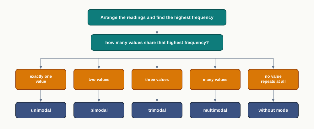
Fig. 2.3 – Classifying distributions by their mode.
The possibility of two modes, or none, is exactly why the mode is used less often than the mean or median: it does not always return a single, clean answer. But where the question really is about what is most common — the commonest wage in a workshop, the most frequent household size in a village — the mode is the only average that answers it directly.
2.5 Comparison Of Mean, Median And Mode
Having three averages raises an obvious question: when do they agree, and when do they part company? The answer lies not in the arithmetic but in the shape of the data. The easiest way to see it is to compare the three against a distribution curve — a graph of how often each value occurs.
The Normal Distribution
The normal distribution is the familiar bell-shaped curve. It describes a set of readings in which most observations cluster around the middle value, and the number of readings falls away symmetrically as you move toward either extreme. Many human traits behave this way — intelligence, personality scores and student achievement all tend to be normally distributed. A normal curve can be tall and narrow or low and wide, depending on how variable the data are, but it is always symmetrical. Fig. 2.4 shows one.
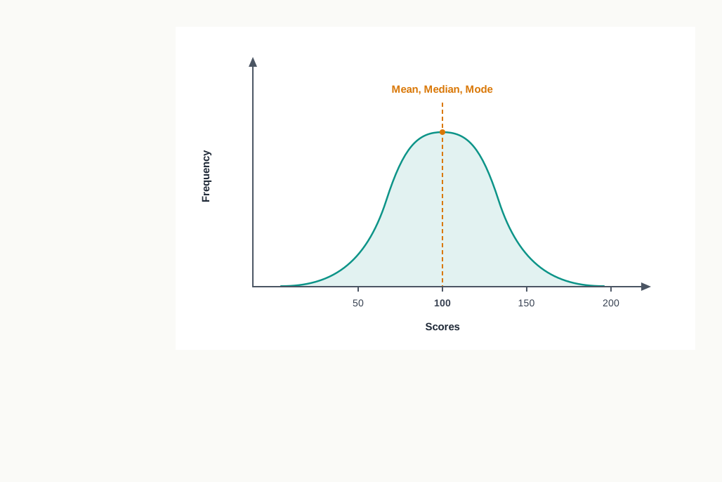
Fig. 2.4 – A symmetrical normal distribution curve.
The symmetry has a striking consequence: in a normal distribution the mean, the median and the mode are all the same value — a score of 100 in Fig. 2.4. The most frequent score sits in the middle, exactly half the readings fall above it and half below, and the bulk of the readings gather around that centre. Very high and very low scores are rare, occurring in the thin tails on either side.
When The Data Are Skewed
Real data are often not symmetrical. When a distribution is skewed — lopsided, with one tail longer than the other — the three averages no longer coincide, and the gap between them tells you which way the data lean. Fig. 2.5 and Fig. 2.6 show the two cases.
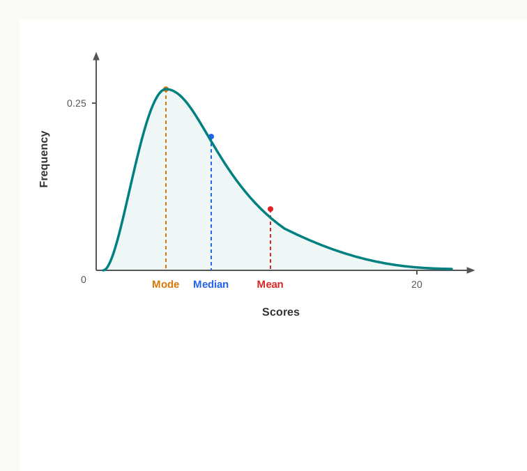
Fig. 2.5 – A positively skewed distribution.
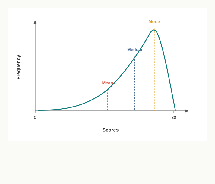
Fig. 2.6 – A negatively skewed distribution.
The pattern is consistent. The mode stays at the peak, where the readings are densest. The mean is dragged toward the long tail by the extreme values it sums in. The median, being positional, lands between the two. So in a positive skew the order runs mode, median, mean from low to high; in a negative skew it reverses to mean, median, mode. Whenever the three separate, the direction of the separation reveals the direction of the skew.
This is also the practical lesson of the whole chapter. Which average best represents a group depends on the group’s shape. For symmetrical data any of the three will do. For skewed data the mean can mislead, and the median often stands in for the typical case more honestly.
2.6 Summary
- Measures of central tendency give a single value that best represents a whole set of readings — the point about which the readings cluster. They are also called statistical averages, and there are three: the mean, the median and the mode.
- The mean is the arithmetic average: the sum of the values divided by the number of values. It uses every reading in the set.
- For ungrouped data the mean can be found by the direct method (add the values and divide) or the indirect method (code the values against an assumed mean, then add the assumed mean back). Both give the same answer; coding just keeps the arithmetic small.
- For grouped data the individual readings lose their identity, so each class is represented by its midpoint. The mean is then Σfx ÷ N by the direct method, or A ± Σfd ÷ N by the indirect method.
- The median is a positional average — the middle value once the readings are placed in order. It splits the series into two equal halves and is independent of the actual extreme values.
- For grouped data the median is located using cumulative frequency and interpolated within the median class by M = l + (i/f)(N/2 − c).
- The mode is the value that occurs most often. It is always a value that actually appears in the data, and a set may be unimodal, bimodal, trimodal, multimodal, or without any mode.
- In a symmetrical, normal distribution the mean, median and mode coincide. In a skewed distribution they separate: the mean is pulled toward the long tail, and the direction of the separation shows the direction of the skew.
- Which average best represents a group depends on the shape of the data — for skewed data the median is often the more honest choice.
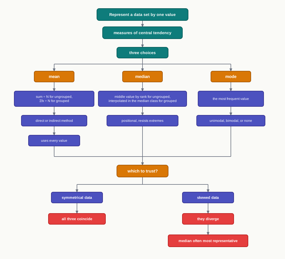
Fig. 2.7 – Summary of central tendency measures.
What This Chapter Cannot Tell You
A single average, of any kind, collapses a whole distribution into one number. It says nothing about how spread out the readings are — how far they vary around the centre. That is the work of the measures of dispersion, which this chapter does not take up.
A grouped-data mean or median rests on assumptions forced by grouping: that readings sit at their class midpoints, or spread evenly within a class. Once data are grouped, these averages cannot recover the original values.
And an average describes only the centre of one set of readings. It cannot tell you whether two things move together — whether more rainfall brings more flooding, for instance. That question belongs to the measures of relationship, the third family named at the very start of the chapter.
2.7 NCERT Questions
- The measure of central tendency that does not get affected by extreme values:
- Mean
- Mean and Mode
- Mode
- Median
- The measure of central tendency always coinciding with the hump of any distribution is:
- Median
- Median and Mode
- Mean
- Mode
Define the mean. (in about 30 words)
What are the advantages of using mode? (in about 30 words)
Explain relative positions of mean, median and mode in a normal distribution and skewed distribution with the help of diagrams. (in about 125 words)
Comment on the applicability of mean, median and mode (hint: from their merits and demerits). (in about 125 words)
Take an imaginary example applicable to geographical analysis and explain direct and indirect methods of calculating mean from ungrouped data.
2.8 Check Your Concepts
Using the wage data in Table 2.3, work out the mean daily wage by the direct method. Show every step, from Σfx to the final figure.
A distribution has two values that share the highest frequency. What is such a distribution called, and what does the presence of two modes suggest about the readings?
When data are grouped, each class is represented by its midpoint in computing the mean. Explain why this is necessary, and state the assumption it forces on the data.
The median is unaffected by an extreme value, but the mean is not. Explain why, referring to how each of the two is found.
From Table 2.4, identify the median class and state the values of l, f, c and i. Explain how the cumulative-frequency column was used to locate that class.
In the indirect method for the grouped wage data, the positive values of fd add to 1060 and the negative values to −800. Show how these give Σfd, then complete the mean using A ± (Σfd ÷ N), with A = 100 and N = 99.
In Fig. 2.5 the mean lies furthest to the right of the three averages. Which readings pull it there, and what is the resulting left-to-right order of mode, median and mean called?