Chapter 3: Graphical Representation Of Data
In the late summer of 1854, cholera swept through a crowded district of London called Soho. People fell ill within hours, and no one agreed on why. Most doctors of the day blamed bad air rising from the streets. A physician named John Snow suspected the water instead — but a suspicion is not proof, and the deaths, written out as a plain list of names and addresses, pointed nowhere in particular.
So Snow did something simple. He took that same list and marked each death as a small stroke on a street map of the neighbourhood, one stroke for each person who had died. As the marks built up, a shape appeared that no column of names could have shown. The deaths were not scattered evenly across Soho. They crowded tightly around a single public water pump on Broad Street, and thinned out with distance from it.
The map turned a list into an argument. Snow persuaded the local authorities to remove the pump’s handle so it could no longer be used, and the outbreak in that pocket of the city faded. He had invented no new fact. Every death on the map was already in his list. What the map added was a pattern the eye could read at a glance — which is the whole business of this chapter.
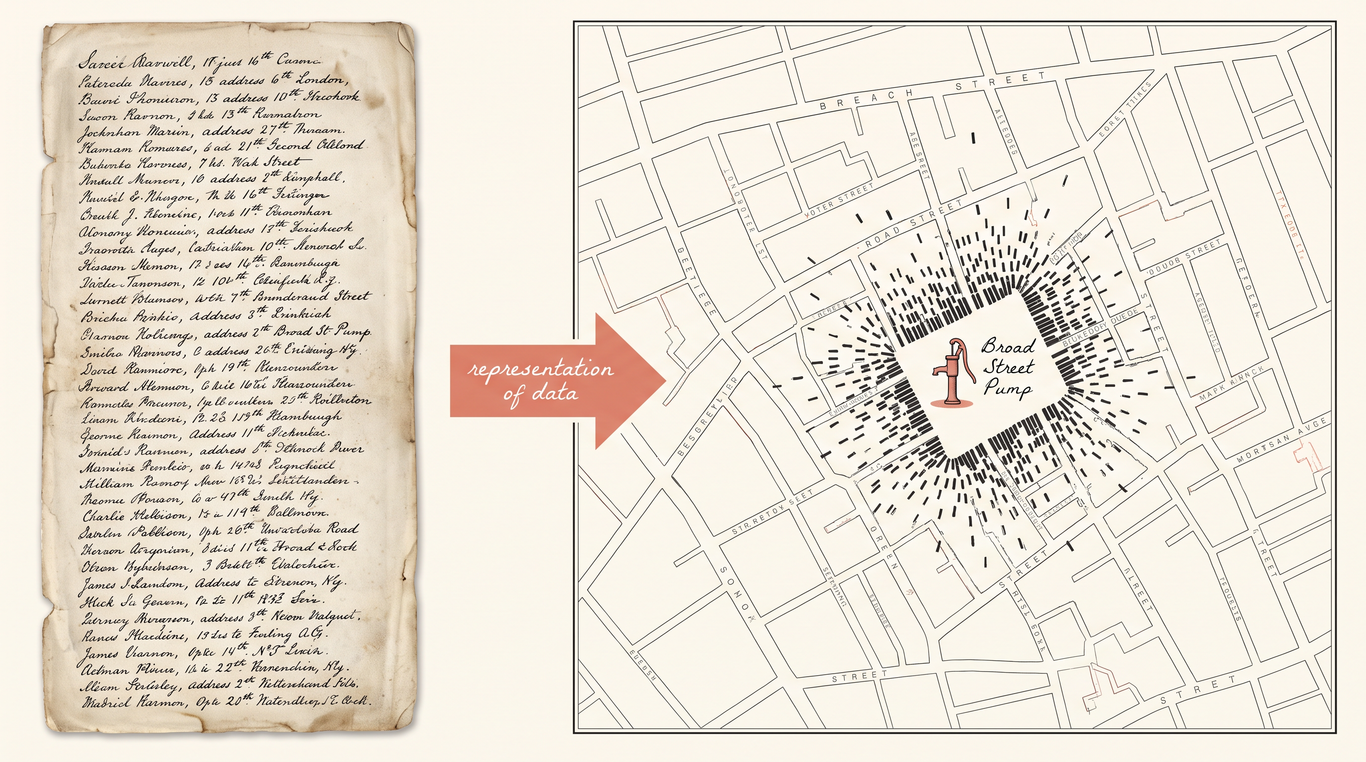
Fig. 3.0 – The Soho cholera deaths map and list.
3.1 Representation Of Data
You have almost certainly seen information drawn as a graph, a diagram or a map rather than written out in words. In the Class 11 book Practical Work in Geography, Part-I, for instance, a set of thematic maps — maps that each show one kind of information across an area — display the relief and slope, the climate, the distribution of rocks and minerals, the soils, the population, the industries, the general land use and the cropping pattern of Nagpur district, in Maharashtra in central India.
Every one of those maps rests on a large body of figures. The figures were first collected, then compiled — gathered into an orderly form — and then processed, meaning worked on until they were ready to use, whether sorted, totalled or converted into rates.
Now imagine the same information set out instead as a long table of numbers, or as a paragraph of description. It would be very hard to form any visual impression from either, and slow to draw an inference. Reading down a column, the eye meets one value at a time and holds nothing. A map or a graph presents all the values together, so a pattern in them can be seen at once.
What Representation Means
The word data needs pinning down first. Data are the recorded facts that describe the properties of whatever we are studying — the rainfall of a place, the population of a state, the price of a crop. They are collected from a variety of sources, as the first chapter of this book discussed, and geographers, economists, resource scientists and decision-makers all rely on large quantities of them.
Data can be kept in a table. But they can also be turned into a picture. Representation of data is the transformation of data through visual methods — graphs, diagrams, maps and charts. A table stores the numbers; representation reshapes them into a form the eye reads as a shape, a trend or a spread.
Why We Bother
Once data are drawn, comparisons become easy, time is saved, and a simplified view of the main features stands out. There is a Chinese proverb that a picture is equivalent to thousands of words, and the graphic method works in exactly that spirit. It also fixes the pattern in memory: a shape that is seen leaves a longer imprint on the mind than a column of figures that is read.
This is why so much of geography is drawn rather than listed. The patterns the subject cares about — how a population grows over time, how it is distributed and how densely, its sex ratio, its age–sex composition, the occupational structure of a territory — are all patterns that a well-chosen graph or map makes visible in a single glance. The rest of this chapter is about how each of those pictures is built.
3.2 General Rules For Drawing Graphs, Diagrams And Maps
Before any single diagram is built, three decisions settle whether it will actually communicate: which method to use, what scale to draw it at, and how to design it so that a reader can decode it unaided. These general rules hold for every graph, diagram and map in this chapter.
3.2.1 Selection Of A Suitable Method
Data carry many different themes — temperature, rainfall, the growth and distribution of population, and the production, distribution and trade of commodities. Each theme has a method of representation that suits it best, and choosing the right one is the first task.
Data that change over time, such as temperature or the growth of population across different periods and for different countries or states, are best shown with a line graph — a graph that plots each value as a point and joins the points with a line, so the rise and fall over time reads as a single moving shape.
Rainfall totals or the production of commodities are best shown with bar diagrams, columns of equal width whose heights stand for the values. Separate quantities like these are compared most easily as columns set side by side.
The distribution of population — human or livestock — and of crop-producing areas suits a dot map, on which equal-sized dots are scattered to show where, and how thickly, a thing occurs. Population density suits a choropleth map, on which each administrative unit is shaded according to its value.
3.2.2 Selection Of Suitable Scale
The scale is the fixed measure that ties the size drawn on the page to the actual value in the data — how many centimetres of bar, or of map strip, stand for one unit of the quantity. Because it governs every plotted value, it must be chosen with the whole data set in view, from the smallest figure to the largest.
The rule is that the scale should be neither too large nor too small. Too large, and the biggest values run off the sheet; too small, and real differences shrink until the eye can no longer tell them apart. A scale that holds the entire range comfortably on the page is the one to keep.
3.2.3 Design
Design is a genuine cartographic task — the same care set out under ‘Essentials of Map Making’ in the Class 11 book Practical Work in Geography, Part-I. A few components must appear on every finished diagram or map, so that a stranger can read it without help.
3.2.3.1 Title
The title names the area shown, the reference year of the data, and the caption of the diagram. These are set in letters and numbers of different sizes and weights, and their placing matters: the title, its subtitle and the year normally sit centred at the top of the map or diagram.
3.2.3.2 Legend
The legend, also called the index, explains every colour, shade, symbol and sign used, and must correspond exactly to the contents of the map or diagram. Without it the shading and symbols are mute. It is normally placed at the lower left or lower right of the map sheet.
3.2.3.3 Direction
A map represents part of the earth’s surface, so it must be oriented to the directions. The direction symbol — the North arrow — is drawn and properly placed, so the reader knows which way the ground actually lies.
3.3 Construction Of Diagrams
Data have measurable characteristics — length, width and volume — and the diagrams and maps drawn to represent them are grouped by how many of these dimensions they use. One-dimensional diagrams, which stand for a value by a single length, include the line graph, the poly graph, the bar diagram, the histogram (a column graph of how often each value occurs) and the age–sex pyramid (back-to-back bars of males and females by age group). Two-dimensional diagrams, which use an area, include the pie diagram and the rectangular diagram. Three-dimensional diagrams, which use a volume, include cube and spherical diagrams.
There are too many of these to construct them all here. The chapter takes up the ones most commonly drawn: line graphs, bar diagrams, the pie diagram, the wind rose and star diagram, and flow charts. Of these, the line graph, the bar diagram, the pie diagram and the flow chart are worked through step by step below.
3.3.1 Line Graph
A line graph is usually drawn for time series data — values recorded for the same thing at successive points in time, such as temperature, rainfall, population growth, birth rates and death rates. Because the points follow one another in time, joining them with a line turns the whole run of values into one rising and falling shape.
The data for the worked example are given in Table 3.1. Here growth rate means the percentage by which the population changed over the decade ending in each year — a positive figure for an increase, a negative one for a fall.
The line is built in a fixed order. First, the data are simplified into round numbers to make plotting easier — the growth rates for 1961 and 1981, for instance, may be rounded to 2.0 and 2.2 while the exact figures in the table stay on record. Next, the two axes are drawn: the time variable (years or months) goes on the X-axis, and the quantity to be plotted (the growth in per cent, or the temperature in °C) goes on the Y-axis. Then a suitable scale is chosen and labelled on the Y-axis; where the data include a negative value, the scale must run below zero to show it, as in Fig. 3.1. Finally, each year’s value is marked with a dot at the right height, and the dots are joined by a free-hand line.
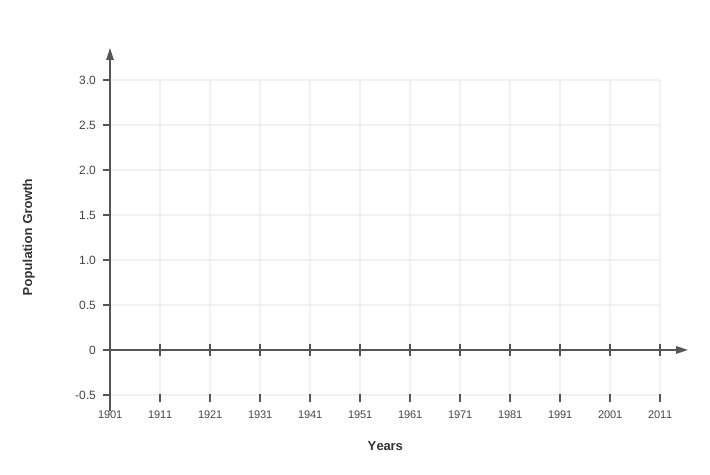
Fig. 3.1 – Construction of a line graph.
When the values are plotted and joined, the finished graph appears as Fig. 3.2. One feature stands out at once: the line dips below zero at 1921. That single negative growth rate marks the one decade in the series when India’s population actually fell.
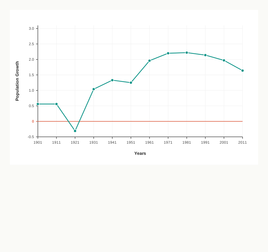
Fig. 3.2 – Annual growth of population in India, 1901–2011.
The chapter sets a task at this point: look at Fig. 3.2 and find out why the population changed so sharply between 1911 and 1921, when the rate swung from a rise to a fall.
3.3.1.1 Polygraph
A polygraph is a line graph carrying two or more lines at once, so several things can be compared on the same frame — the growth rates of different crops like rice, wheat and pulses, or the birth rates, death rates, life expectancy or sex ratio of different states or countries. The lines are told apart by pattern: a straight line, a broken line, a dotted line, a mixed dot-and-dash line, or lines of different colours.
The worked example compares the sex ratio — the number of females per 1000 males — of three states across six census years, using the data in Table 3.2.
Plotted as three separate lines on one frame, the data become Fig. 3.3, and the three states’ paths can be followed and compared at a glance.
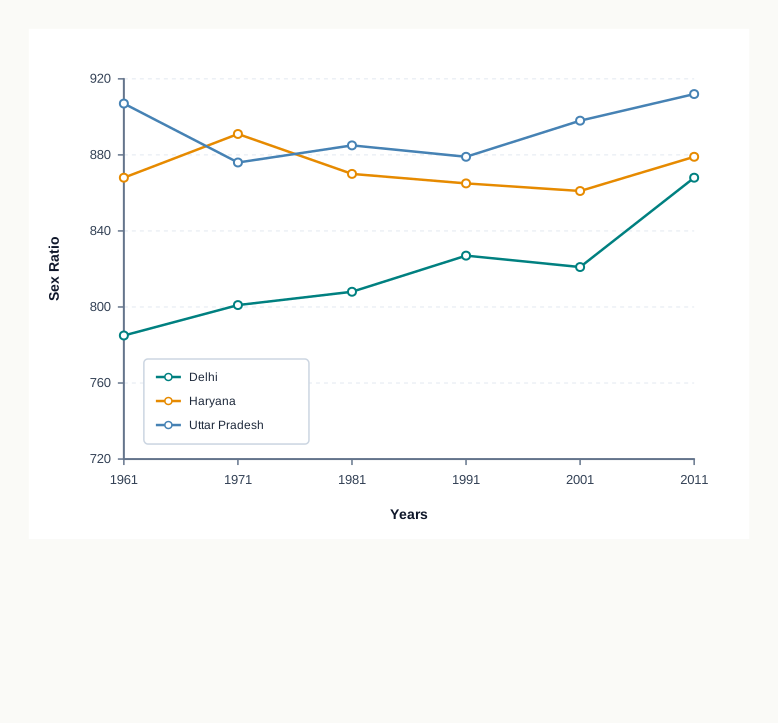
Fig. 3.3 – Sex-ratio of selected states, 1961–2011.
3.3.2 Bar Diagram
A bar diagram is drawn as columns of equal width, which is why it is also called a columnar diagram. Three rules govern it: every bar has the same width, the bars are set at equal intervals, and they may be shaded with colours or patterns to keep them distinct. Depending on the data, a bar diagram may be simple, compound or a polybar.
3.3.2.1 Simple Bar Diagram
A simple bar diagram is built for a quick comparison. It helps to arrange the data in ascending or descending order before plotting — though time-series data are always kept in their time order instead. The worked example uses the monthly rainfall of Thiruvananthapuram, the capital of Kerala on India’s south-west coast, from Table 3.3.
To draw it, the axes are set on graph paper, the Y-axis is marked in intervals of 5 cm to carry the rainfall, and the X-axis is divided into twelve equal parts for the twelve months. Each month’s rainfall is then plotted as a bar to the chosen scale, giving Fig. 3.4. The tall June bar and the low February one make the wet and dry months obvious without any need to scan the numbers.
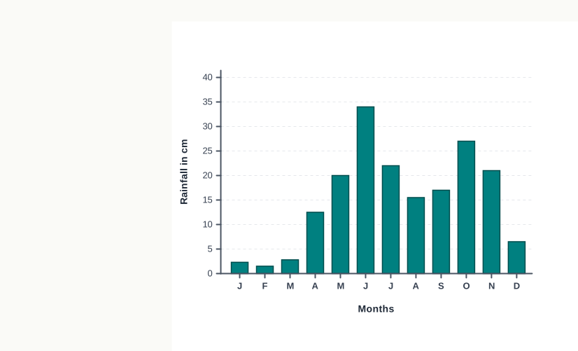
Fig. 3.4 – Average monthly rainfall of Thiruvananthapuram.
3.3.2.2 Line And Bar Graph
Two closely linked characteristics — most often the mean monthly temperature and rainfall of a place — can be shown together by combining a line and bars in one diagram. The months run along the X-axis, and the two Y-axes carry different quantities on the two sides: rainfall on the left, temperature on the right. The worked example uses Delhi’s data from Table 3.4.
The X-axis is divided into twelve parts for the months. The right-hand Y-axis is scaled in equal steps of 5 °C or 10 °C for temperature; the left-hand Y-axis in equal steps of 5 cm or 10 cm for rainfall. Temperature is then drawn as a line and rainfall as bars, producing Fig. 3.5. In one frame, the reader sees Delhi hold its heat through the summer while its rain arrives only with the July–August monsoon.
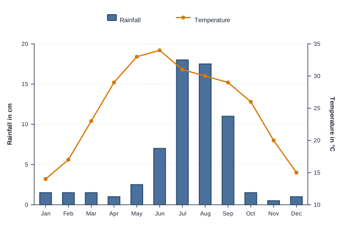
Fig. 3.5 – Temperature and rainfall in Delhi.
3.3.2.3 Multiple Bar Diagram
A multiple bar diagram sets two or more variables side by side for comparison — for instance the share of males and females in the total, rural and urban population, or the share of canal, tube-well and well irrigation in different states. The worked example shows the decadal literacy rate — the percentage of people able to read and write, as counted by the census — for total population, males and females, from Table 3.5.
Time runs along the X-axis and the literacy rates up the Y-axis. For each census year, three columns are plotted close together — total, male and female — so the gap between the male and female bars can be read directly. Fig. 3.6 shows the result: every group climbs across the decades, and the female bar, though lowest throughout, closes much of the distance on the male bar by 2011.
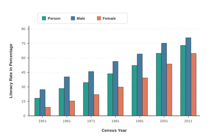
Fig. 3.6 – Literacy rate in India, 1951–2011.
3.3.2.4 Compound Bar Diagram
A compound bar diagram puts the parts of a whole inside a single bar, one rectangle stacked on another, so that both the total and its breakdown show together. The worked example uses India’s gross electricity generation, split into thermal, hydro and nuclear, from Table 3.6.
After arranging the data, one bar is drawn for each year, its full height standing for the total generation, and that height is divided into thermal, hydro and nuclear segments. Fig. 3.7 shows the outcome: the bars grow taller year on year as total generation rises, while the thermal segment towers over the small hydro and nuclear slices in every bar.
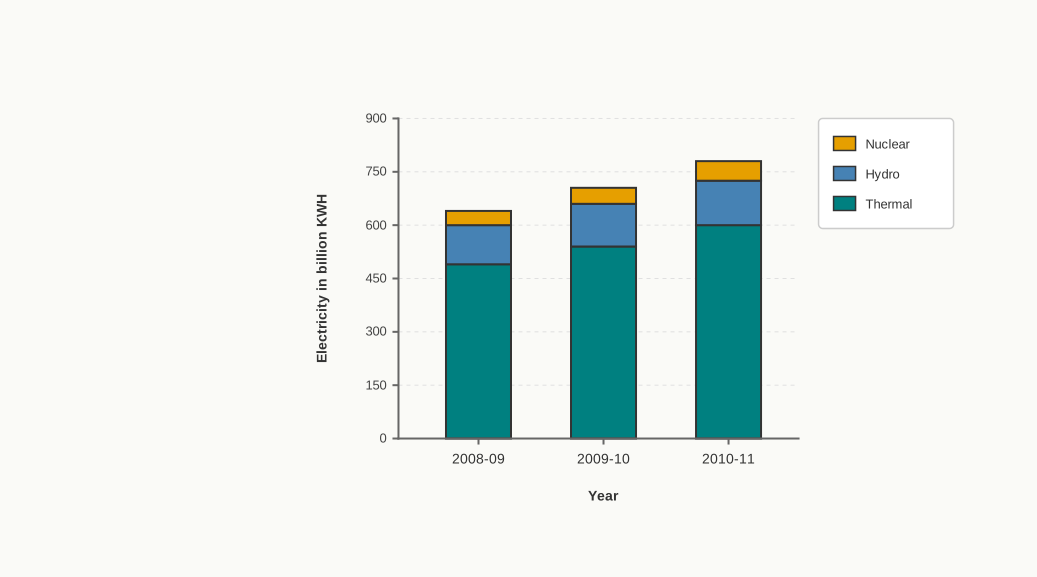
Fig. 3.7 – Gross electricity generation in India.
3.3.3 Pie Diagram
A pie diagram, also called a divided circle diagram, shows the whole of a quantity as a full circle, then splits the circle into sectors whose angles are proportional to the parts. The whole circle is 360°, so each part’s share of the total becomes its share of 360°.
The angle for any part is found from its value:
\[\text{Angle of a sector} = \frac{\text{Value of the given State/Region} \times 360}{\text{Total Value of All States/Regions}} \quad (\text{in degrees})\]
where the value and the total are in the same units (rupees, tonnes, persons, and so on), and the answer is an angle in degrees.
When the data are already in percentages, the total is 100, so the formula simplifies:
\[\text{Angle of a sector} = \frac{\text{Percentage of } x \times 360}{100} \quad (\text{in degrees})\]
Since 360 ÷ 100 = 3.6, every percentage is simply multiplied by the constant 3.6 to get its angle. The worked example represents India’s export shares from Table 3.7 (a).
Each percentage is multiplied by 3.6 to get its angle, giving Table 3.7 (b). For example, Asia and ASEAN’s 56.2 per cent becomes 56.2 × 3.6 = 202.32, rounded to 203° — a sector larger than a semicircle on its own.
To draw the circle, a suitable radius of 3, 4 or 5 cm is chosen and a radius line drawn from the centre to the edge. The sectors are then measured off clockwise in ascending order of angle, starting with the smallest, so that small measuring errors do not pile up on the last and biggest sector — which is exactly why one starts small rather than large. Finally the title, subtitle and legend are added, each category given a distinct shade. The finished circle is Fig. 3.8, on which the single Asia-and-ASEAN sector fills more than half the pie.
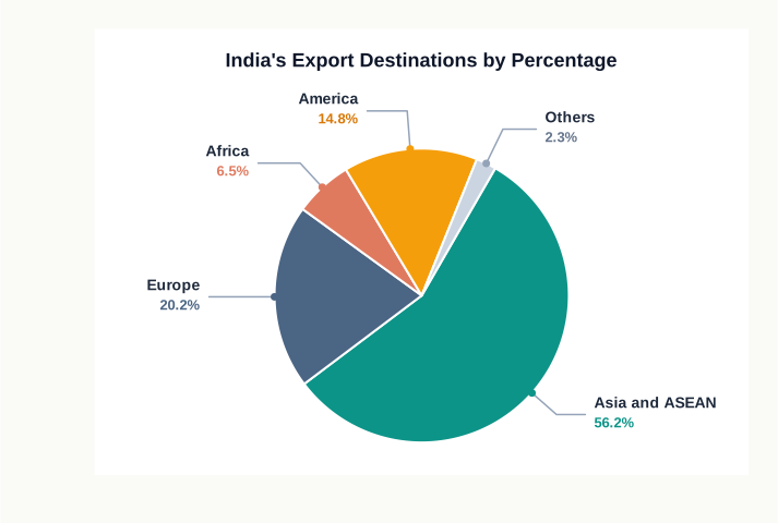
Fig. 3.8 – Direction of Indian exports, 2010–11.
3.3.4 Flow Maps/Chart
A flow chart is a combination of a graph and a map, drawn to show the flow of goods or people between places of origin and destination; because it captures movement, it is also called a dynamic map. A transport map showing the number of passengers or vehicles is the clearest example. The flows are drawn as lines whose width is proportional to the quantity — so a thicker line means heavier traffic. Such maps generally represent either the number and direction of vehicles, or the number of passengers and quantity of goods carried.
Preparing one needs three things: a route map showing the transport routes and their connecting stations; the data on the flow — goods, passengers or vehicle numbers, with origin and destination; and a scale to convert those quantities into line widths. The worked example maps the trains running on selected routes of Delhi and its adjoining areas, from Table 3.8.
The first step is to take an outline map of Delhi and its adjoining areas showing the railway lines and nodal stations, as in Fig. 3.9. The next is to fix a scale that turns train numbers into strip widths.
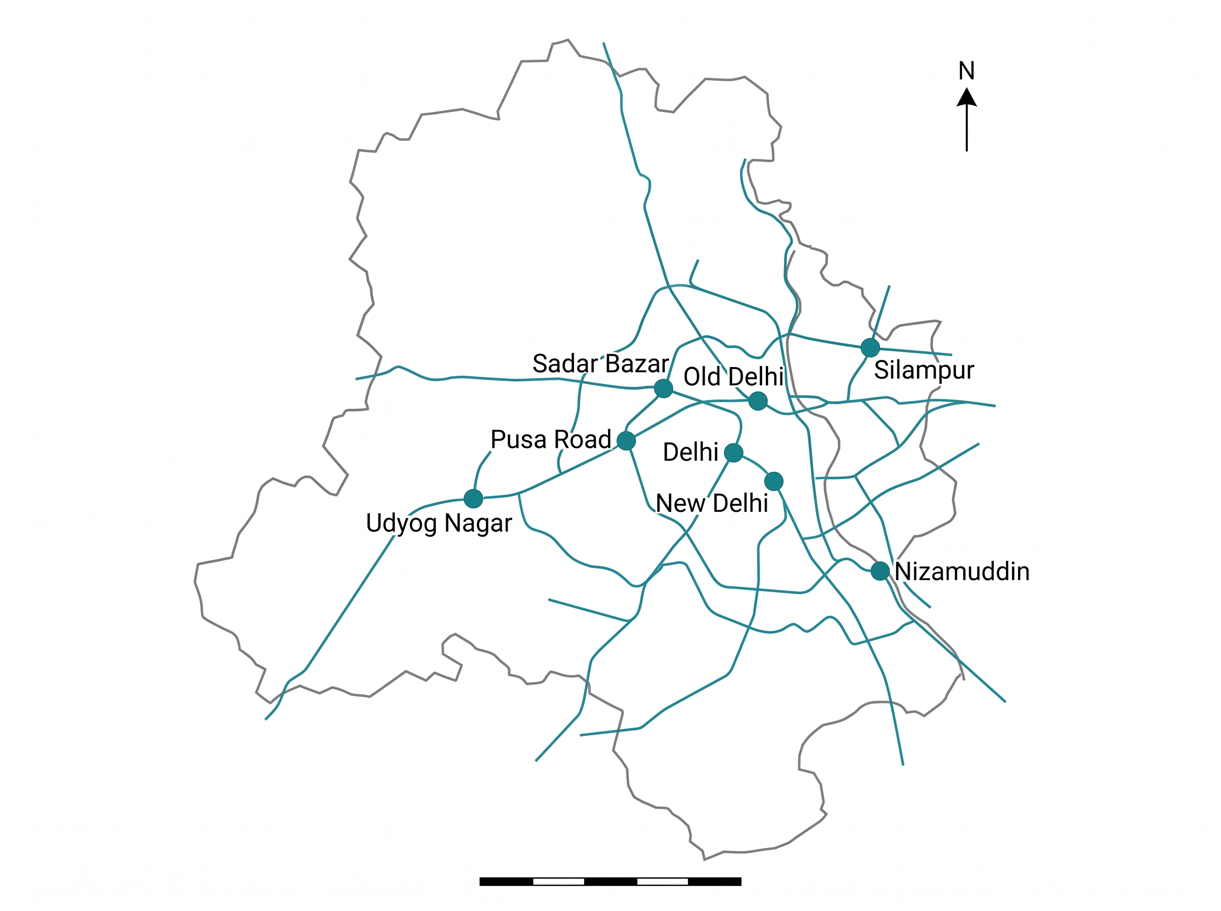
Fig. 3.9 – Map of Delhi and adjoining areas.
The scale works because width now carries meaning: a reader can rank the whole rail network by traffic just by comparing thicknesses, with no numbers to read. The 10 mm Old Delhi–New Delhi strip is instantly the busiest corridor, and the 1.2 mm Udyog Nagar–Tikri Kalan strip the quietest — the eye sorts sixteen routes at a glance. Each route’s strip is then plotted between its stations, and a terraced scale is added as the legend, with a distinct symbol marking the nodal stations, giving Fig. 3.10.
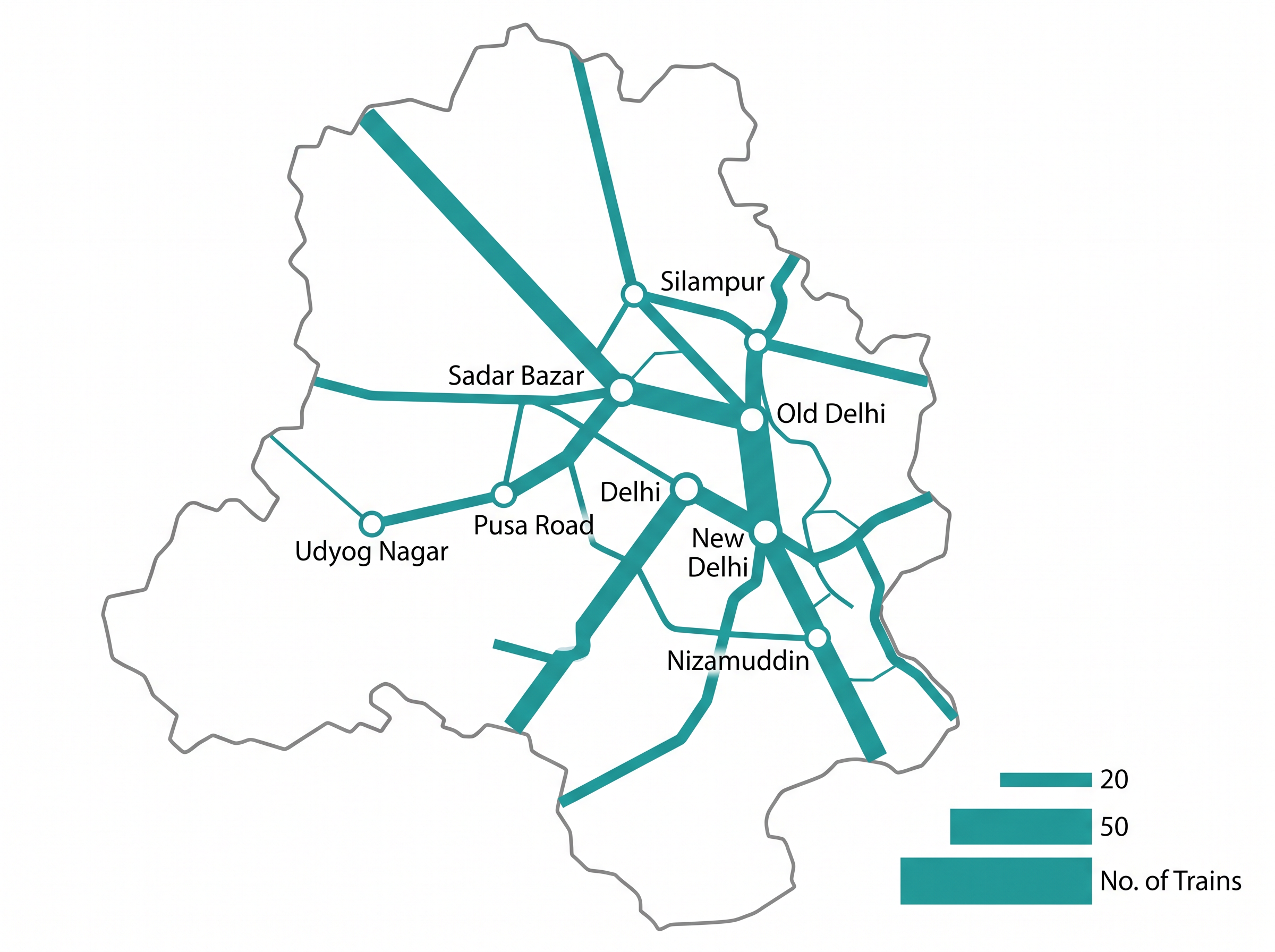
Fig. 3.10 – Railway traffic flow map of Delhi.
The same method maps water, not trains. In a flow map of the Ganga basin — the drainage basin of the river Ganga across the northern plains of India — each channel’s strip is drawn in proportion to the water it carries, measured in cusecs (a cusec is a flow of one cubic foot of water per second). Fig. 3.11 gives the basin with the flow figures in thousands of cusecs, and taking a scale of a 1 cm-wide strip for 50,000 cusecs turns it into the constructed flow map, Fig. 3.12, where the trunk channel swells downstream as tributary after tributary adds its flow.
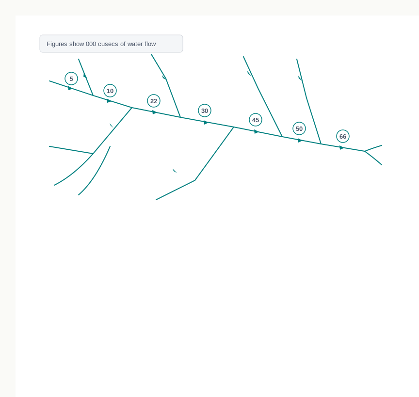
Fig. 3.11 – The Ganga basin flow figures.
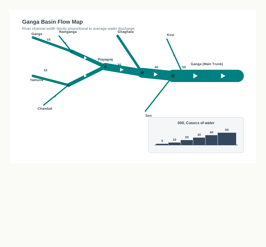
Fig. 3.12 – Construction of a flow map.
3.3.5 Thematic Maps
Graphs and diagrams compare the internal variations within a set of data well, but they cannot show where those variations sit on the ground — they miss the regional picture. To recover it, geographers draw thematic maps, and because each one shows how a single theme is spread across space, these are also called distribution maps.
Making one needs three inputs: state- or district-level data on the chosen theme; an outline map of the study area with its administrative boundaries; and a physical map of the region — a physiographic map for population distribution, or a relief-and-drainage map for a transport map.
The drawing must be planned so that the finished map carries five things a reader needs: the name of the area, the title of the subject-matter, the source of the data and its year, an indication of the symbols, signs, colours and shades used, and the scale. With those in place, the remaining decision is which method of thematic mapping to use — the subject of the next section.
3.4 Classification Of Thematic Maps Based On Method Of Construction
Thematic maps fall into two broad kinds by what they measure. Quantitative maps, also called statistical maps, show the actual variations within the data — for example maps that divide an area into belts receiving more than 200 cm, 100 to 200 cm, 50 to 100 cm, and less than 50 cm of rainfall. Non-quantitative maps, also called qualitative maps, show characteristics that cannot be measured on a number scale — for example a map that simply marks high and low rainfall areas without stating the amounts.
There are many ways to build these maps; this section works through three quantitative methods: dot maps, choropleth maps and isopleth maps.
3.4.1 Dot Maps
A dot map shows the distribution of something countable — population, cattle, a crop — by scattering equal-sized dots across the administrative units, so that where the dots crowd together, the thing is dense, and where they thin out, it is sparse.
Building one needs an administrative map showing state, district or block boundaries; statistical data on the theme for each unit; a scale fixing how much one dot stands for; and a physiographic map, especially relief and drainage, so the dots can be placed sensibly. Two precautions matter: the boundary lines between units should be kept thin, not thick and bold, and every dot must be exactly the same size, since the dot’s size is what carries the scale.
The worked example maps India’s population in 2001, using Table 3.9.
The number of dots for each state comes straight from its population and the value of a dot.
That single division is repeated for every state, and each state then receives its number of dots. But the dots are not spread evenly across the state’s outline: the relief map is consulted so that mountainous, desert and snow-covered tracts, where few people live, are given fewer dots. This is what makes the finished map, Fig. 3.13, read as a true picture of where people actually are — dense across the northern plains, thin over the western desert and the high mountains.
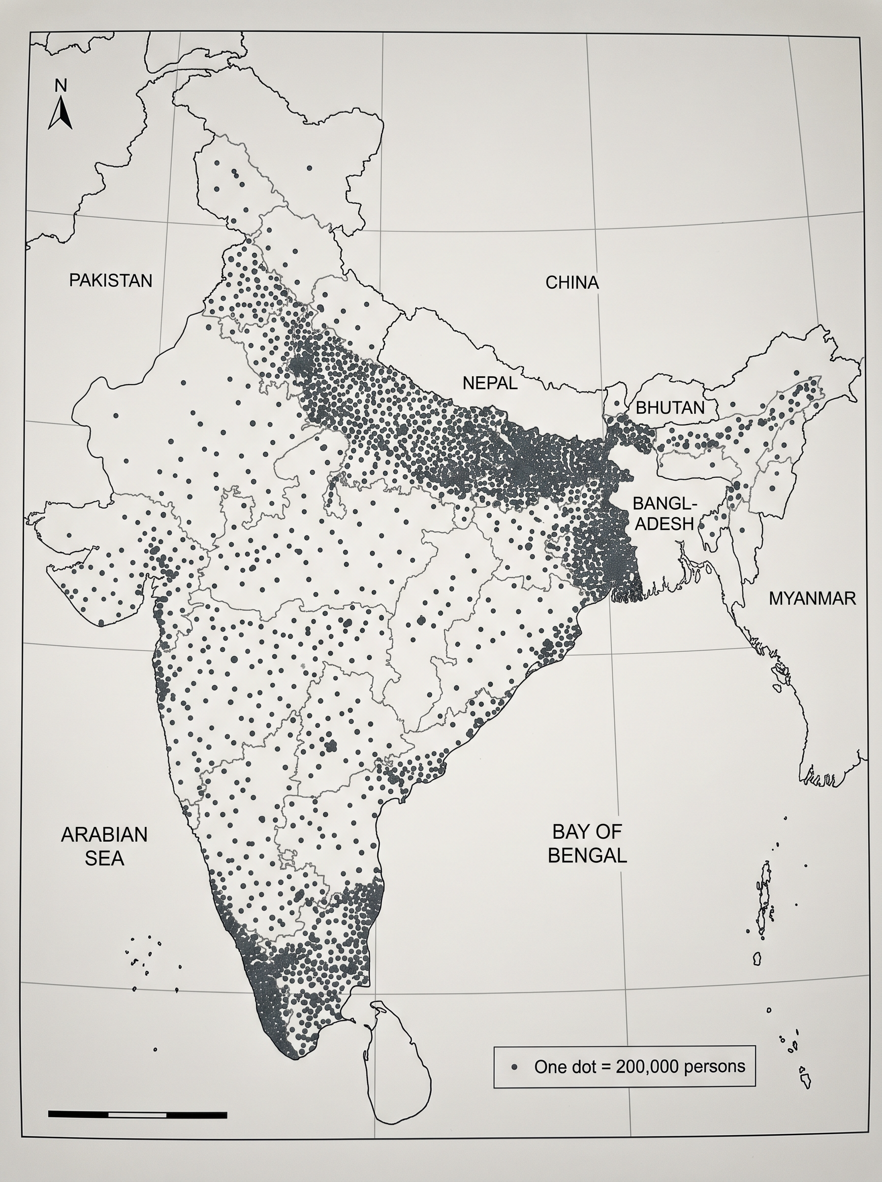
Fig. 3.13 – Population of India, 2001.
3.4.2 Choropleth Map
A choropleth map also works on administrative units, but instead of scattering dots it shades each whole unit according to its value. It suits rates and ratios rather than raw counts — the population density (the number of people per unit of area), literacy or growth rates, and the sex ratio. It needs only two things: a map of the area showing its administrative units, and the matching statistical data for each unit.
The method runs in steps. The data are first arranged in ascending or descending order. They are then grouped into five categories — very high, high, medium, low and very low. The width of each category, the interval, is fixed by dividing the range by five, where the range is the largest value minus the smallest. Finally, shades or colours are assigned in order, darker for higher, lighter for lower. The worked example maps India’s literacy rates for 2001, from Table 3.10.
The categories are fixed by a short calculation on the sorted data.
Each band gathers the states whose rate falls inside it. The very low band, 47–56, holds Bihar, Jharkhand, Arunachal Pradesh, and Jammu and Kashmir. The low band, 56–65, holds Uttar Pradesh, Rajasthan, Andhra Pradesh, Meghalaya, Odisha, Assam, Madhya Pradesh and Chhattisgarh. The medium band, 65–74, holds Nagaland, Karnataka, Haryana, West Bengal, Sikkim, Gujarat, Punjab, Manipur, Uttarakhand, Tripura and Tamil Nadu. The high band, 74–83, holds Himachal Pradesh, Maharashtra, Delhi and Goa, and the very high band, 83–92, holds Mizoram and Kerala. Each band is then given a shade from light to dark and the map is completed with its design attributes, giving Fig. 3.14.
The map converts a long column of numbers into a pattern the eye reads at once — a literate south and a less literate belt across the east and centre. But that same shading carries a cost, which the reading box makes plain.
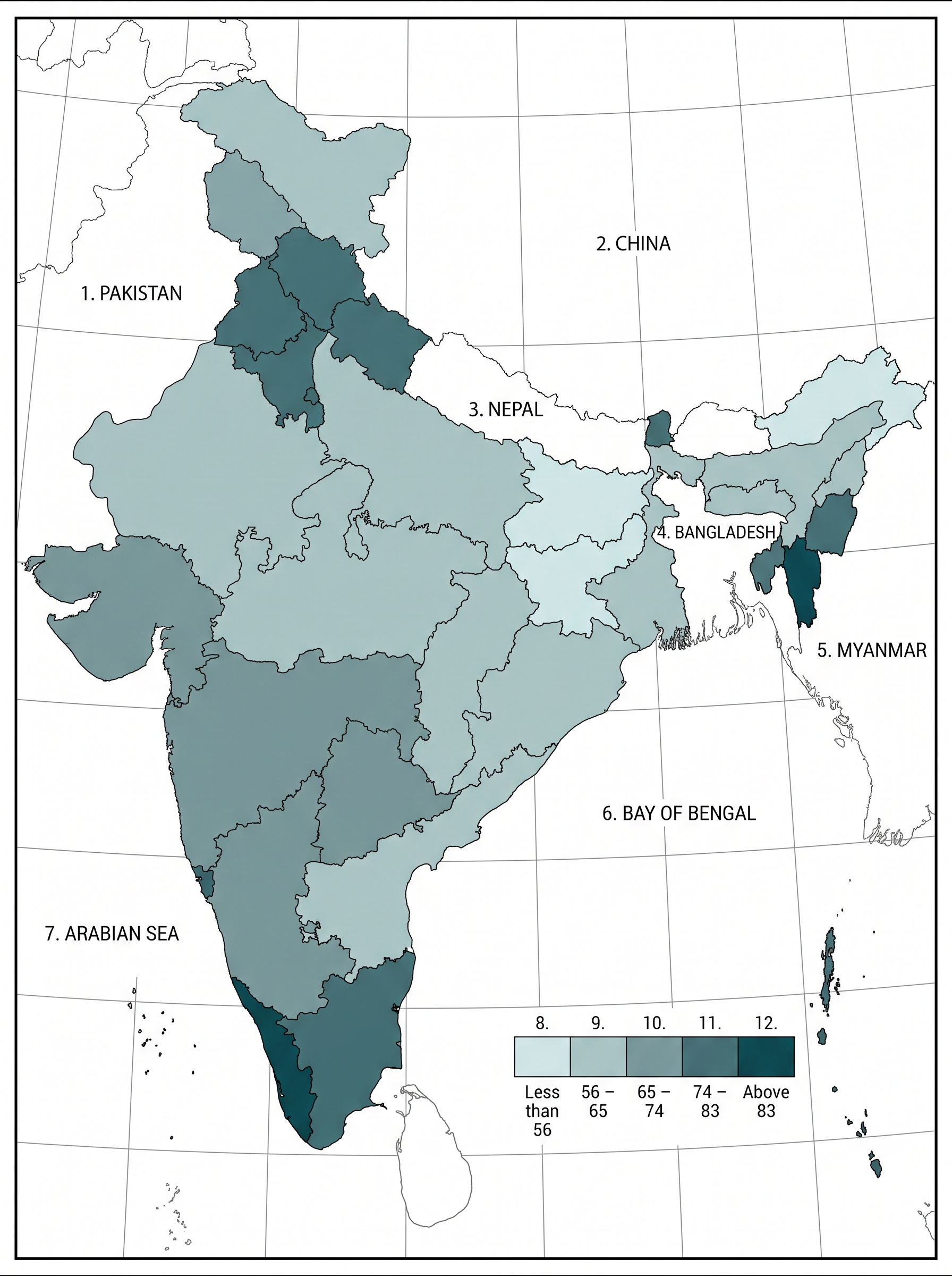
Fig. 3.14 – Literacy rate of India, 2001.
3.4.3 Isopleth Map
Choropleth maps follow administrative boundaries, but many geographical facts — slope, temperature, rainfall — vary continuously across the land, ignoring any border. An isopleth map handles these by drawing lines that join places of equal value. The word comes from iso, meaning equal, and pleth, meaning lines. The family is large and each member joins equal values of one thing: the isotherm (equal temperature), the isobar (equal pressure), the isohyet (equal rainfall), the isoneph (equal cloudiness), the isohel (equal sunshine), the contour (equal height), the isobath (equal depth) and the isohaline (equal salinity).
Drawing one requires a base map showing the point locations of the observing places, data on temperature, pressure or rainfall over a definite period, and a smooth drawing instrument such as a French curve. Three rules hold: an equal interval of values is chosen; an interval of 5, 10 or 20 is usually ideal; and each isopleth’s value is written along the line, on either side or in a break in the middle.
Interpolation
Because a line of equal value rarely passes exactly through an observing station, its position between stations has to be estimated. Interpolation is this insertion of intermediate values between two observed values — say the temperatures recorded at two stations, or the spot heights of two points. To interpolate, the smallest and largest values on the map are found, their range is taken (maximum minus minimum), and a whole-number interval such as 5, 10 or 15 is chosen. The exact point at which an isopleth crosses the line between two stations is then fixed by a formula:
\[\text{Point of Isopleth} = \frac{\text{Distance between the two points (in cm)}}{\text{Difference between the two values of the corresponding points}} \times \text{Interval}\]
Here the distance is measured on the map in centimetres, the difference is between the two stations’ recorded values, and the interval is the gap between the value being drawn and the nearer station’s value.
The point where each isopleth belongs is found this way all across the map; the isopleth of the minimum value is drawn first, and the others follow in order. Joining the points of equal value gives the finished lines, as in the stages of Fig. 3.15, where a scatter of spot readings is turned first into interpolated points and then into smooth isopleths and shaded belts.
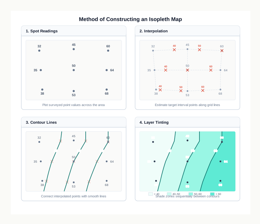
Fig. 3.15 – Drawing of isopleths.
3.5 Summary
Representation of data means transforming numbers into a visual form — graphs, diagrams, maps and charts — so that patterns become visible, comparisons become easy, time is saved, and the picture stays longer in memory than a column of figures.
Before drawing anything, three choices are made: a suitable method for the theme, a suitable scale that is neither too large nor too small, and a proper design carrying a title, a legend and a direction.
A line graph shows time series data as points joined into one moving shape; a polygraph puts two or more such variables on the same graph, each as its own line, for direct comparison.
A bar diagram compares quantities as columns of equal width: a simple bar diagram for one set of values, a multiple bar diagram for grouped bars side by side, and a compound bar diagram for parts stacked within one bar. A line-and-bar graph pairs temperature and rainfall on two scales in a single figure.
A pie diagram, or divided circle, shows the parts of a whole as slices, each slice’s angle being its percentage multiplied by 3.6.
A flow map, also called a dynamic map, shows movement between places by drawing each route as a line whose width is proportional to the quantity carried.
Thematic, or distribution, maps show a single theme across space. They are quantitative when they map measured variation and non-quantitative when they map described differences.
A dot map shows counted distributions with equal dots of a fixed value; a choropleth map shades whole units by their rate or density in graded classes; an isopleth map joins places of equal value with lines placed by interpolation, for a field that changes continuously.
The whole chapter reduces to a single question — what does the data show, and which picture shows it best — which the master flowchart lays out as a branching choice.
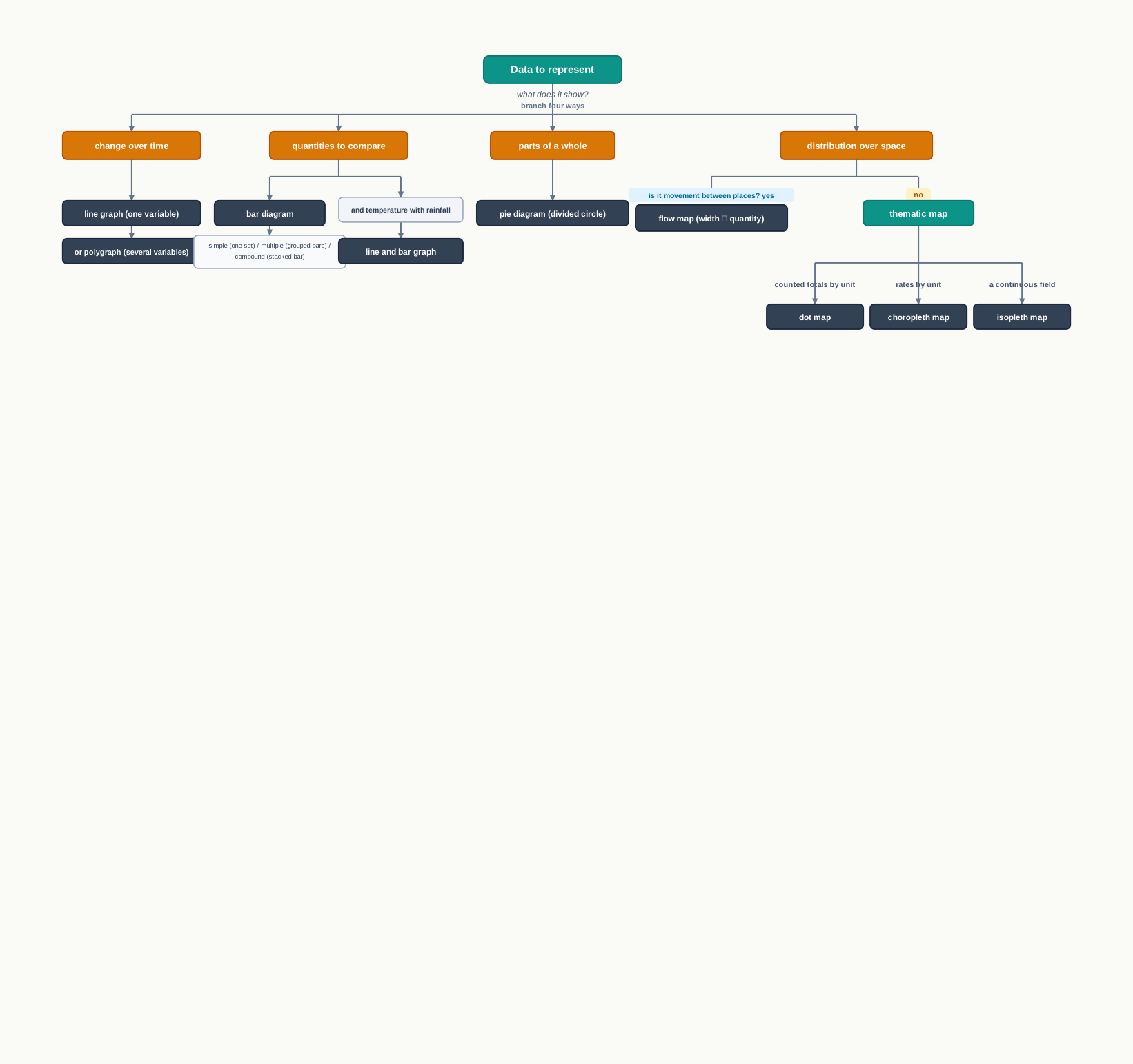
Fig. 3.16 – Choosing the right diagram for data representation.
What This Chapter Cannot Tell You
- A chosen picture is only as current as the year printed on its data: the tables here rest on figures for years such as 2001, 2010–11 and 2011, and a fresher census or survey would redraw them.
- Every method hides something by design. A choropleth shade averages a whole unit and buries the districts inside it; a class boundary is a choice, so two units nine points apart can share one colour; a line drawn between two census years is drawn, not measured; and an interpolated isopleth is a reasoned estimate of the space between stations, not a record of it.
- These are methods for showing a pattern, not for explaining it. The map can reveal where literacy is low or where trains run thickest, but why it is so lies outside the drawing.
3.6 NCERT Questions
- Which one of the following maps shows the population distribution?
- Choropleth maps
- Isopleth maps
- Dot maps
- Square root maps
- Which one of the following is best suited to represent the decadal growth of population?
- Line graph
- Bar diagram
- Circle diagram
- Flow diagram
- Polygraph is constructed to represent:
- Only one variable
- Two variables only
- More than two variables
- None of the above
- Which one of the following maps is known as ‘Dynamic Map’?
- Dot map
- Choropleth
- Isopleth
- Flow map
What is a thematic map? (in about 30 words)
Differentiate between multiple bar diagram and compound bar diagram. (in about 30 words)
What are the requirements to construct a dot map? (in about 30 words)
Describe the method of constructing a traffic flow map. (in about 30 words)
What is an Isopleth map? How is interpolation carried out? (in about 30 words)
Describe and illustrate the important steps to be followed in preparing a choropleth map. (in about 30 words)
Discuss the important steps to represent data with the help of a pie-diagram. (in about 30 words)
Represent the following data with the help of a suitable diagram — India: Trends of Urbanisation 1901-2001.
| Year | Decennial growth (%) |
|---|---|
| 1911 | 0.35 |
| 1921 | 8.27 |
| 1931 | 19.12 |
| 1941 | 31.97 |
| 1951 | 41.42 |
| 1961 | 26.41 |
| 1971 | 38.23 |
| 1981 | 46.14 |
| 1991 | 36.47 |
| 2001 | 31.13 |
- Represent the following data with the help of a suitable diagram — India: Literacy and Enrolment Ratio in Primary and Upper Primary Schools.
| Year | Literacy Ratio — Person | Male | Female | Enrolment Primary — Boys | Girls | Total | Enrolment Upper Primary — Boys | Girls | Total |
|---|---|---|---|---|---|---|---|---|---|
| 1950-51 | 18.3 | 27.2 | 8.86 | 60.6 | 25 | 42.6 | 20.6 | 4.6 | 12.7 |
| 1999-2000 | 65.4 | 75.8 | 54.2 | 104 | 85 | 94.9 | 67.2 | 50 | 58.8 |
- Represent the following data with the help of a pie-diagram — India: Land use 1951-2001.
| 1950-51 | 1998-2001 | |
|---|---|---|
| Net Sown Area | 42 | 46 |
| Forest | 14 | 22 |
| Not available for cultivation | 17 | 14 |
| Fallow Land | 10 | 8 |
| Pasture and Tree | 9 | 5 |
| Cultruable Waste Land | 8 | 5 |
- Study the table given below and draw the given diagrams/maps — Area and Production of Rice in major States.
| States | Area in 000 ha | % to total area | Production 000 tones | % to total production |
|---|---|---|---|---|
| West Bengal | 5,435 | 12.3 | 12,428 | 14.6 |
| Uttar Pradesh | 5,839 | 13.2 | 11,540 | 13.6 |
| Andhra Pradesh | 4,028 | 9.1 | 12,428 | 13.5 |
| Punjab | 2,611 | 5.9 | 9,154 | 10.8 |
| Tamil Nadu | 2,113 | 4.8 | 7,218 | 8.5 |
| Bihar | 3,671 | 8.3 | 5,417 | 6.4 |
- Construct a multiple bar diagram to show area under rice in each State.
- Construct a pie-diagram to show the percentage of area under rice in each State.
- Construct a dot map to show the production of rice in each State.
- Construct a choropleth map to show the percentage of production of rice in States.
- Show the following data of temperature and rainfall of Kolkata with a suitable diagram.
| Months | Temperature in °C | Rainfall in cm |
|---|---|---|
| Jan. | 19.6 | 1.2 |
| Feb. | 22.0 | 2.8 |
| Mar. | 27.1 | 3.4 |
| Apr. | 30.1 | 5.1 |
| May | 30.4 | 13.4 |
| June | 29.9 | 29.0 |
| Jul. | 28.9 | 33.1 |
| Aug. | 28.7 | 33.4 |
| Sep. | 28.9 | 25.3 |
| Oct. | 27.6 | 12.7 |
| Nov. | 23.4 | 2.7 |
| Dec. | 19.7 | 0.4 |
3.7 Check Your Concepts
In Fig. 3.2, identify the decade in which India’s population growth rate fell below zero, and explain in one line what a negative growth rate means for the size of the population.
The chapter defines both quantitative and non-quantitative thematic maps. State how the two differ, and give one example of each drawn from the chapter.
Set out, in order, the four steps for constructing a line graph.
A dot map and a choropleth map both show how something is distributed across administrative units. Explain the difference in what each one places on a unit to carry its value.
Table 3.9 fixes one dot as 100,000 persons. Using this, calculate the number of dots for Rajasthan, whose population is 56,473,122, and check your answer against the figure in the table.
Using the pie-diagram formula, calculate the angle of the Europe slice from Table 3.7 (a), where Europe is 20.2 per cent of India’s exports. Show the arithmetic.
In the chapter’s isotherm example, two stations read 28 °C and 33 °C and lie 10 mm apart on the map. Using the interpolation formula, find how far from the 28 °C station the 30 °C isotherm should be drawn.
A choropleth map shades an entire state in a single colour for its literacy rate. State one thing such a map cannot tell you about literacy within that state, and one reason why its class boundaries are a choice rather than a fixed fact.