Chapter 4: Spatial Information Technology
A district office keeps its knowledge of the land in a wooden drawer. A soil map, a road map, a map of the villages, a map of where the wells run dry each May. Each was drawn by a different hand, in a different year, at a different scale. Each answers one question and no more.
One morning a simple request arrives. A new primary health centre is to be built, and someone must decide where. The honest answer needs several maps read together at once — which villages lie far from any existing centre, which sit near a motorable road, which fall inside the belt that floods every monsoon. On paper the maps will not line up. Traced onto sheets and stacked on a light table, they slip and blur. To shift the proposed site by two kilometres and see who is now within reach, the whole tracing must be redrawn from the beginning.
This is the wall that paper maps hit. A map shows what someone once chose to show, frozen at the moment it was printed. It cannot be questioned, only replaced.
A Geographical Information System takes those same maps, stores each as a layer of located data, and lets you put to them the questions the drawer could never answer: what is where, why is it there, and what changes if it moves.
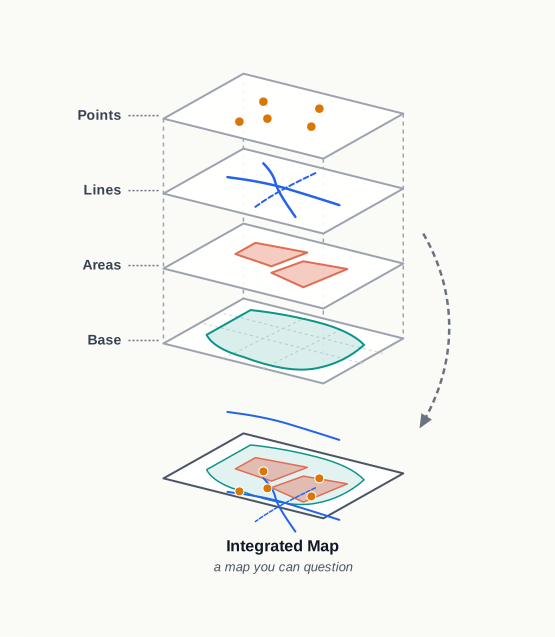
Fig. 4.0 – Stacked map layers in a GIS.
4.1 What Is Spatial Information Technology?
You already know that a computer makes short work of tasks that once took days by hand. It sorts and counts large volumes of data, and it draws the graphs, diagrams and maps that turn that data into a picture. Two established fields rest on exactly this power.
A Database Management System, or DBMS, is the set of principles and methods for storing, processing and retrieving data using computer hardware together with application software. Its partner, Computer Assisted Cartography, is the making of maps and diagrams by that same combination of machine and software. Between them they can take a mass of raw figures and return an ordered table or a finished map.
But there the power stops. A DBMS processes data, and computer cartography presents it — and that is all. Neither can take the processed data or the printed map and use it to reach a decision. The map tells you what is there; it cannot tell you what to do about it. A tool that could do that is called a decision support system — a system that helps a person choose between options by testing them against the data.
The Questions A Map Cannot Answer
Think of the questions we meet in ordinary life and expect real answers to. What is where? Why is it there? What will happen if it is shifted to a new location? Who will be benefited if it is moved? Who stands to lose the benefit if the move takes place? A printed map holds a great deal of information, yet on its own it answers none of these.
To answer them, you have to gather the necessary data from many different sources and bring them together inside a computer fitted with geo-processing tools — software that can work on data according to where things sit on the ground. A system built to do this is a Spatial Information System. This chapter sets out its basic principles and follows it into its best-known form, the Geographical Information System, or GIS.
What ‘Spatial’ Means
The word spatial comes from space, and it points to features and phenomena spread across a space you can define on the ground and measure. Anything spatial therefore has real, physical dimensions — a length, an area, a position you could survey.
Most of the data we handle today carry a spatial component, which is simply a location. The address of a municipal office is a location; the boundary of an agricultural holding is a location. Once data is tied to a place on the Earth, it becomes spatial.
Spatial Information Technology is the use of technological inputs to collect, store, retrieve, display, manipulate, manage and analyse this spatial information. It is not a single tool but a joining of several. As shown in Fig. 4.1, it brings together Remote Sensing (measuring the Earth from a distance, by satellite or aircraft), GPS (the satellite system that fixes a position on the ground), GIS, Digital Cartography (map-making done wholly on the computer) and Database Management Systems.
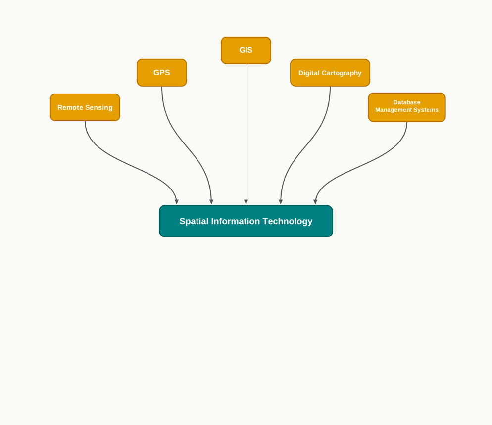
Fig. 4.1 – Components of spatial information technology.
4.2 What Is GIS (Geographical Information System)?
The advanced computing systems that became available from the mid-1970s could do something new. They could process georeferenced information — information tied to a known position on the Earth — and use it to organise spatial and attribute data together, integrate them, locate specific records in separate files, run computations, perform analysis, and so build a decision support system.
A system able to do all of this is a Geographic Information System, or GIS. NCERT defines it precisely: a system for capturing, storing, checking, integrating, manipulating, analysing and displaying data which are spatially referenced to the Earth. In practice this means a computer database in which every record is tied to a location, worked on by suitable application software. The new power is not the drawing or the storing, both of which older tools could do; it is the integration — pulling records from separate files together because they share a place.
Like the wider technology it belongs to, a GIS is an amalgamation — here, of Computer Assisted Cartography and the Database Management System. It also borrows ideas and methods from a wide circle of subjects: Computer Science, Statistics, Cartography, Remote Sensing, Database Technology, Geography, Geology, Hydrology, Agriculture, Resource Management, Environmental Science and Public Administration. That breadth is the point — a system meant to answer real questions about the land has to draw on every field that studies the land.
4.2.1 Forms Of Geographical Information
Geographical information takes two forms, and a GIS needs both. Spatial data is data that fixes a location — where something is on the ground. Attribute data, also called non-spatial data, describes that thing without itself being a location: its name, its size, its class, its value.
The Shapes Spatial Data Takes
Spatial data shows up in three forms of appearance — positional, linear and areal (Fig. 4.2). A positional feature is a point — a single located spot, such as a survey benchmark. A linear feature is a line — something long and thin, such as a river. An areal feature is an area — a patch with a boundary, such as a lake.
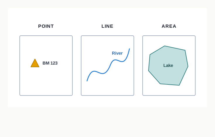
Fig. 4.2 – Forms of spatial data: point, line and area.
Every one of these located shapes carries attribute data alongside it. The point is not just a dot; it is a benchmark of a certain height. The river is not just a line; it has a name and a flow. This pairing — a shape with a location, plus a set of facts describing it — is what a plain picture cannot hold, and what a GIS is built to keep together.
Telling The Two Apart
The clearest way to see the difference is to lay two records side by side. Consider first a cycle shop’s stock register (Table 4.1). It lists parts by number, quantity and description. None of it is spatial: a wheel spoke or a tyre could be sitting in any shop anywhere, so nothing in the record pins it to a place.
Now consider a record of male and female literacy across four states in 1981 (Table 4.2). This record is spatial, because one of its columns — the state — names a place with a definite location on the map. Attach the literacy figures to those locations and the data can be used in a GIS; the cycle-shop list cannot, because it has no place to be attached to. A database, in short, holds attributes and their values, but only the record whose attribute is a location is spatial.
Getting Data Into A GIS
Before any of these data forms can be stored, they must be geometrically registered — fitted to a single agreed coordinate system, a grid of reference lines that gives every point a unique address on the Earth’s surface — and then coded so the GIS can hold them in its internal structure. The spatial data are the single most important prerequisite of the whole system; without a location to hang on, the attribute data has nowhere to go.
The spatial data at a GIS’s core can be built in three ways. You can acquire ready-made data in digital form from a data supplier. You can digitise existing analogue data — that is, convert paper records into digital form. Or you can carry out your own surveys of the features on the ground. Section 4.6 returns to these routes in detail.
Which route you choose is governed by three things: the application itself, meaning what the GIS is for; the budget available; and the type of data structure you need, vector or raster — the two ways of storing spatial data taken up in Section 4.5.
For most users the commonest source of spatial data is a map — either a topographical map, which shows the general lie of the land (its relief, drainage, roads and settlements), or a thematic map, which shows a single subject such as soils or population. The map may be in hard copy on paper or soft copy on a computer. Every such map shares three features: a definite scale, which fixes the relationship between distance on the map and distance on the ground; symbols and colours, which stand for the attributes of the things mapped; and an agreed coordinate system, which locates those things on the Earth.
4.3 Advantages Of GIS Over Manual Methods
A printed map is an honest, careful thing. It has geometric fidelity — it stays faithful to the true shapes, distances and directions of the ground it represents, to the limit of its scale. Yet however well it is drawn, a paper map is born with three limitations.
First, its information is processed and presented in one particular way — the way its maker chose. You receive their decisions about what to include and how to show it, not answers to your own questions. Second, a map is drawn for one or more predetermined themes; the themes were fixed before printing, so the map cannot take on a subject it was never designed to carry. Third, to alter anything the map shows, a whole new map must be drawn — there is no editing a printed sheet, only replacing it.
What A GIS Adds
A GIS is built the other way round. It stores the data separately from the way the data is shown, and it can present the same data in several forms. That separation is the source of its advantages.
A user can interrogate the spatial features on the screen — click a feature and call up the attribute data attached to it, ready for analysis. The relationship even runs backwards: instead of only reading a finished map, you can query or analyse the attribute data and have the GIS draw a map as the answer. Spatial operations such as polygon overlay or buffering, which Section 4.6 sets out, can be run across the integrated database to generate wholly new sets of information that were present in no single layer. And because records share a common location code, different items of attribute data can be linked to one another through the place they have in common.
4.4 Components Of GIS
A GIS is a system, and like any system it is more than its machine. It stands on five components working together — hardware, software, data, people and procedures (Fig. 4.3). Leave out any one and the system does not run.
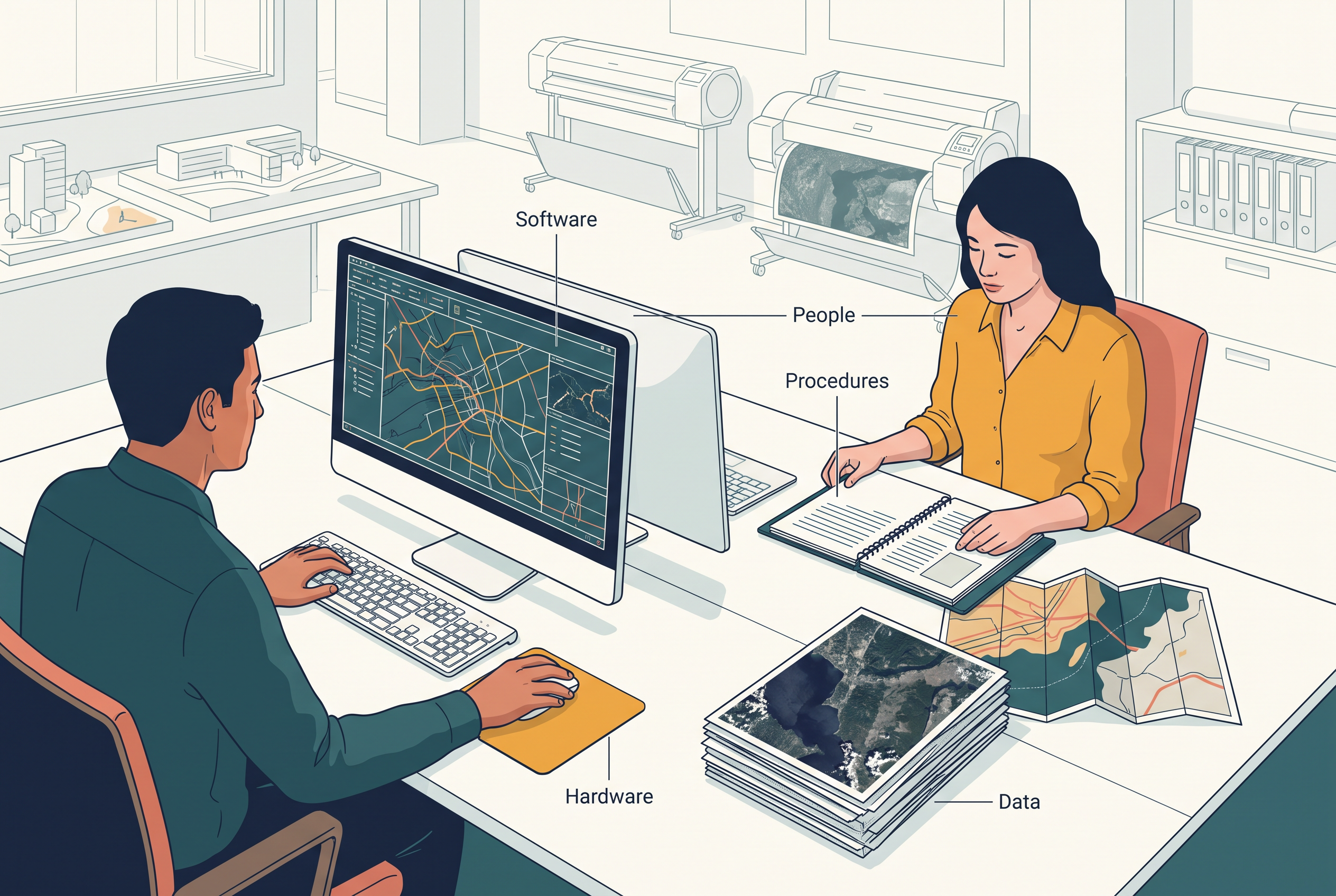
Fig. 4.3 – The five components of a GIS.
4.4.1 Hardware
At the level of major parts, a GIS rests on three: the hardware, the software modules, and a database management system that keeps the data organised. The hardware itself is the physical machinery — the sub-systems that handle processing, storage, display, and the input and output of data. The software modules carry out data entry, editing, maintenance, analysis, transformation, manipulation, display and output, while the DBMS looks after how all the data is arranged.
4.4.2 Software
The software is the working heart of a GIS, and a usable system needs application software with three kinds of functional module — a functional module being a part of the program built to do one job. One module handles data entry, editing and maintenance. A second handles analysis, transformation and manipulation. A third handles the display and output of the data.
4.4.3 Data
Spatial data, together with the tabular data attached to it, is the backbone of a GIS. That data may be bought ready-made from a supplier, or created and collected in-house by the user. The digital map is the basic input; tabular data describing the objects on that map can be attached to it. A GIS then integrates this spatial data with other data resources, and can draw on a DBMS to do so.
4.4.4 People
A GIS is only as useful as the people who run it, and they range widely — from the hardware and software engineers who build and maintain it, to the resource and environmental scientists, the policy-makers, and the agencies that monitor and carry out decisions. This cross-section of people uses the GIS to build a decision support system and to solve real problems as they arise.
4.4.5 Procedures
Procedures are the agreed steps that tell everyone how the data is to be handled — how it will be retrieved, input into the system, stored, managed, transformed, analysed and finally presented as an output. They set out the path a set of data follows through the GIS from beginning to end (Fig. 4.4).

Fig. 4.4 – The path of data through a GIS.
4.5 Spatial Data Formats
Spatial data can be stored in two quite different formats — raster and vector. A raster stores a feature as a pattern of small squares; a vector stores it as a set of lines drawn between fixed points. The same piece of ground can be held either way, and the choice shapes everything that follows.
4.5.1 Raster Data Format
Picture a single line drawn diagonally across a sheet of paper. To store it as a raster, the computer lays a fine grid over the paper — like graph paper — and divides it into a matrix of small squares called cells. Each cell is given a position in the data file and a value that records the attribute found at that spot; in picture form, one cell is one pixel. Because every cell carries a row number and a column number, any single pixel can be pinned down by its row-and-column coordinates (Fig. 4.5). From this grid of valued cells the original image can be rebuilt or viewed.
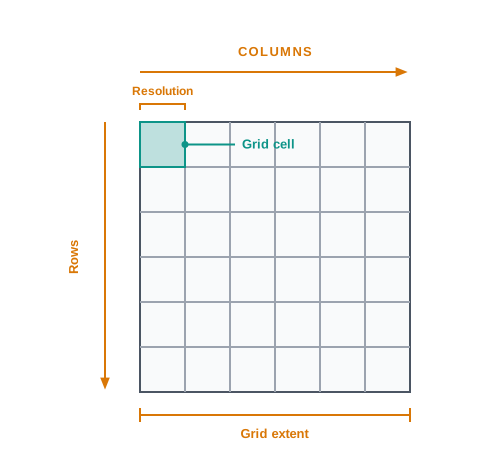
Fig. 4.5 – Generic structure of a raster grid.
The Size Of The Cell
How good the raster is depends on how fine the grid is. The link between the size of each cell and the number of cells is called the resolution of the raster (Fig. 4.6). Make the cells smaller and you get more of them, and the picture grows sharper.
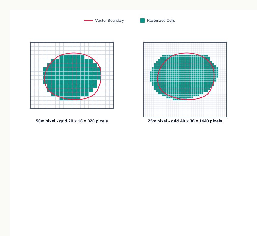
Fig. 4.6 – Effect of raster grid size on shape accuracy.
Those two numbers are the whole idea of resolution. Smaller cells trace the outline more closely, so the 1440-pixel image looks sharper and truer than the 320-pixel one. But the detail is paid for: about four and a half times as many cells to store and handle. Choosing a cell size is really choosing where to sit on that trade-off between sharpness and size.
Where Raster Works Best
Raster formats suit some jobs far better than others. They are the natural choice for the digital form of aerial photographs, satellite images and scanned paper maps; for work where costs must be kept low; where the map needs no analysis of individual features; and where a plain ‘backdrop’ map is all that is wanted behind other information.
4.5.2 Vector Data Format
Now store that same diagonal line as a vector. Instead of filling squares, the computer records the coordinates of the line’s start and end points and joins them. Each point is written as two or three numbers — X and Y for a flat, two-dimensional map, with Z added for three dimensions (Fig. 4.7). X is the distance of the point from the left edge of the sheet, Y its distance from the bottom edge, and Z its height above or below the sheet. Join the measured points and you have the vector.
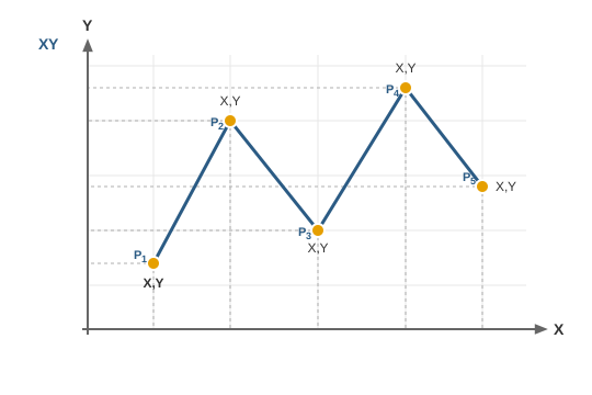
Fig. 4.7 – The vector data model.
A vector model stores its points by their real coordinates on the Earth. Lines are built from points taken in a set order, and that order gives each line a direction; areas, or polygons — closed shapes bounded by lines — are built up from points or lines in turn. A vector can also carry topology, a record of how features connect and touch: which lines meet at a junction, which areas share a border. The surest way to enter vector data is manual digitising — tracing features by hand so their coordinates are captured point by point.
Where Vector Works Best
Vector formats earn their place in the opposite kind of task: highly precise applications; situations where file size must be kept small; work that calls for the analysis of individual map features; and cases where descriptive information has to be stored alongside the shapes.
Weighing Raster Against Vector
Each format is strong exactly where the other is weak (Fig. 4.8). Raster’s advantages are a simple data structure, easy and efficient overlaying, compatibility with satellite imagery, an efficient handling of ground that varies sharply from place to place, ease of programming for oneself, and the ability to hold several attributes on the same grid of cells. Against these stand its disadvantages: it uses computer storage inefficiently, introduces errors in the perimeter and shape of features, makes network analysis difficult and projection transformations inefficient, and loses information when the cells are large, giving less accurate — though still interactive — maps.
Vector’s balance is the mirror image. Its advantages are a compact data structure, efficiency in network analysis, efficient projection transformation, and accurate map output. Its disadvantages are a complex data structure, difficult overlay operations, an inefficient handling of ground that varies sharply, and no compatibility with satellite imagery. Figure 4.8 sets the same point, line, area, network and surface side by side in both formats, so the difference can be seen at a glance.
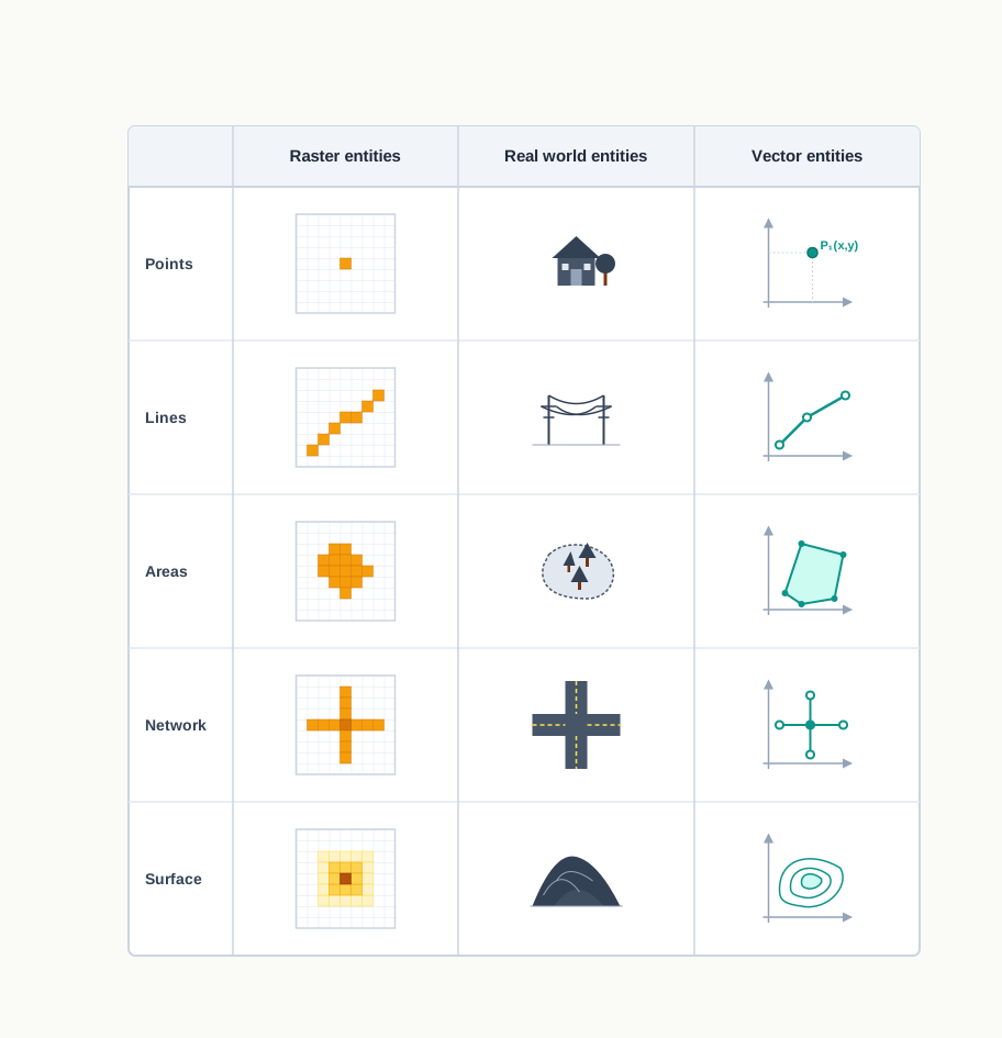
Fig. 4.8 – Spatial features in raster and vector formats.
4.6 Sequence Of GIS Activities
Building and using a GIS is not one act but a chain of them, done in a fixed order. Five activities make up the work: spatial data input, entering the attribute data, data verification and editing, the linking of spatial and attribute data, and finally spatial analysis (Fig. 4.9). Each stage feeds the next, so an error early on travels all the way down the line.
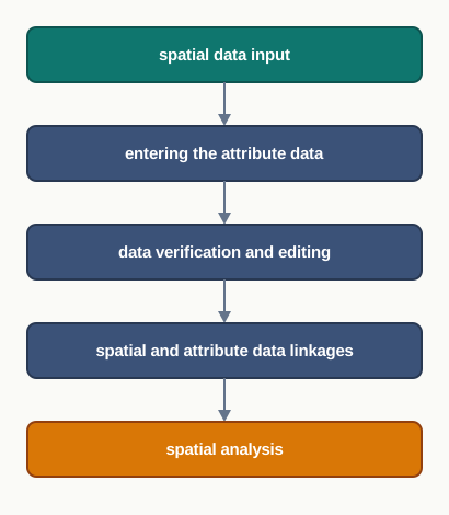
Fig. 4.9 – The five activities of GIS work.
4.6.1 Spatial Data Input
The spatial database at the heart of a GIS can be built from many sources. These fall into two broad categories: buying ready-made digital data from a supplier, or creating the digital data yourself by hand.
4.6.1.1 Acquiring Digital Data Sets From A Data Supplier
Today’s data suppliers offer digital data of every kind, from small-scale maps of large regions to large-scale plans of small areas. For many local governments and private organisations this is invaluable, freeing them from the labour of digitising or surveying their own data.
Using ready-made data is attractive and saves time, but it carries a danger: data compatibility. When data from different sources are combined in one project, differences in their map projection — the method used to flatten the curved Earth onto a flat sheet — and in their scale, base level and attribute descriptions can all cause trouble. To be sure that bought data fits the job, a user must check its scale; the geo-referencing system it uses; the techniques and sampling strategy behind its collection; the quality of the data; the classification and interpolation methods used, interpolation being the estimating of values for places that lie between the points actually measured; the size and shape of its individual mapping units; and the length of the record.
The problems grow sharpest when data are drawn from many sources and the area of study crosses administrative boundaries. Different referencing systems, classifications and sampling then collide, which is why compiling inter-province and inter-district data sets is so error-prone. Once compatibility is settled, the data are transferred to the GIS from a medium such as DAT tapes, CD-ROMs or floppy disks, and at that point the encoding and structuring of the source must be converted to match the GIS.
4.6.1.2 Creating Digital Data Sets By Manual Input
Feeding data in by hand runs through four main stages: entering the spatial data, entering the attribute data, verifying and editing both, and, where needed, linking the spatial data to the attribute data.
How the data are entered depends on whether the database has a vector topology or a grid-cell raster structure. The two commonest ways of putting spatial data in are digitisation — tracing features into coordinates — and scanning. In the entity model, geographical features are points, lines, polygons or pixels, each defined by a series of coordinates. Those coordinates are read from the map’s or aerial photograph’s own referencing system, or by laying a graticule — the grid of latitude and longitude lines — or a plain grid over it. Digitisers and scanners save enormous time and labour that would otherwise go into writing coordinates down by hand.
4.6.1.3 Scanners
A scanner converts analogue data into a digital, grid-based image. In spatial data capture it turns a line map into a high-resolution raster image, which can be used as it is or processed further into vector topology. There are two basic types: scanners that record data step by step, and scanners that take in a whole document in one pass.
The step-by-step type carries a source of light on a movable arm — usually light-emitting diodes or a stabilised fluorescent lamp — together with a digital camera. The camera’s special sensors, called Charged Coupled Devices (CCDs), are semiconductor devices arranged in an array; they translate the photons of light striking them into counts of electrons, which are then stored as a digital value.
As either the scanner or the map moves, a two-dimensional digital image is built up. The map may sit on a flat bed, over which the light source travels up and down, or on a rotating drum. For large maps the camera and light are fixed on a stand and the map itself is fed past them. Modern document scanners work like laser printers in reverse: their scanning surface is made with a fixed grid of light-sensitive spots that the software can address directly, so there are no moving parts but a single lamp, and the resolution is set by the geometry of that surface and the memory available rather than by any mechanical arm. Even the best scan is never perfect — it carries every smudge and defect of the original — so the excess data must be cleaned out before the image can be used.
4.6.2 Entering The Attribute Data
Attribute data describe the properties of a spatial feature that are not themselves locations. A road, for example, may be captured as a run of raster pixels or as a single vector line, and shown on the map by a chosen colour or symbol. Its kind may be carried in the cartographic symbols, while its other attributes — the road’s width, its surface type, an estimate of its traffic, the traffic rules that apply — are stored separately: as spatial information in the GIS in a relational database, or bound in with the spatial description in an object-oriented database.
Such attribute data rarely have to be typed from scratch. They can be drawn from published records, official censuses, primary surveys or spreadsheets, and fed into the GIS either by hand or by importing them through a standard transfer format.
4.6.3 Data Verification And Editing
Data that has just been captured must be checked before it is trusted, because capture introduces error. Digitisation can leave omissions, or overshoots and undershoots where a line is drawn too far or not far enough. The surest check is to print the captured data on a translucent sheet at exactly the scale of the original, lay the two over each other on a light table, and compare them square by square, working from left to right and top to bottom, marking every gap and misplacement on the print. The errors that show up fall into three kinds.
4.6.3.1 Spatial Data Are Incomplete Or Double
Incompleteness creeps in through omissions when points, lines or areas are entered by hand. In scanned data it appears as gaps between lines, where the raster-to-vector conversion has failed to join all the parts of a single line.
4.6.3.2 Spatial Data At The Wrong Scale
Digitising at the wrong scale simply puts the data in at the wrong scale. In scanned data the same fault arises during geo-referencing, when incorrect values are fed in.
4.6.3.3 Spatial Data Are Distorted
Distortion follows when the base map used for digitising is not true to scale. Aerial photographs are especially prone to it, their scale thrown out by lens distortions, by relief, and by the tilt of the camera. Paper maps and field documents pick up random distortions of their own from rain, sunshine and repeated folding. Where the database’s coordinate system differs from that of the input, the data must be transformed from one system to the other.
All these errors are put right through the editing tools built into most GIS software — a slow, hands-on job that can take longer than the data input itself. The operator views the faulty patch of map on screen and corrects it with the keyboard, a mouse-driven cursor or a small digitiser tablet. A minor misplacement in a vector database can be nudged into place with the cursor; many systems also offer commands to move, rotate, erase, insert, stretch or truncate features, and ‘weeding’ algorithms to strip out the excess coordinate points that clutter a line. In raster data, both attribute and spatial errors are fixed by changing the value of the faulty cells. Only once the spatial errors are gone can the topology of the vector line and polygon networks be generated.
4.6.3.4 Data Conversion
For analysis, every layer in use at once must share a single format — all vector, or all raster. The usual move is from vector to raster, because most analysis is done in the raster domain; the vector data are turned into raster by laying a grid of a chosen cell size over them. The reverse, raster to vector, is done mainly to shrink the data, since raster files need far more storage than vector ones.
4.6.4 Geographic Data: Linkages And Matching
Bringing spatial and attribute data together is one of the most important steps in a GIS, and it must be done with care. Tie attribute data to the wrong spatial data and the whole later analysis collapses into nonsense. Matching one data layer against another matters just as much.
4.6.4.1 Linkages
A GIS routinely links separate data sets. Suppose you want the death rate from malnutrition among children under ten in a state. If one file holds the number of children in that age group and another holds the deaths from malnutrition, the two files must first be linked; only then can one figure be divided by the other to give the rate.
4.6.4.2 Exact Matching
Exact matching is used when one file holds information about a set of features — towns, say — and another file holds further information about the very same towns. A key common to both files, such as the town’s name, lets the GIS pull out the matching record from each and join them into a new combined file.
4.6.4.3 Hierarchical Matching
Some data are gathered in fine detail but only now and then, others broadly but often. Land-use data over a wide area may be collected frequently, while land-transformation data are collected for small areas at longer intervals. If the small areas nest neatly inside the large ones, hierarchical matching adds the small-area figures together until the grouped total matches a large area, and then matches the two exactly.
4.6.4.4 Fuzzy Matching
Often the smaller areas do not fit inside the larger ones at all, a problem that is common with environmental data. Crop boundaries, set by the edges of fields, rarely line up with the boundaries of soil types. To find the most productive soil for a crop, the two must be overlaid and crop productivity worked out for each soil type — laying one map over another and reading off every combination of soil and yield. A GIS can perform all of this, but only when the sets of information relate to the same patch of ground.
4.6.5 Spatial Analysis
The real strength of a GIS lies in analysis, and it is analysis that sets a GIS apart from other information systems. Its analytical functions use both the spatial and the non-spatial data to answer questions about the real world, building and applying models that expose the trends hidden in the data and open up new possibilities. The aim is always to turn raw data into information a decision-maker can use, and even to predict how something will change over space and time. Good analysis begins by naming the problem and fixing the purpose, then proceeds step by step. Four spatial operations are available — overlay analysis, buffer analysis, network analysis and the Digital Terrain Model — of which this chapter takes up the first two.
4.6.5.1 Overlay Analysis Operations
The hallmark of a GIS is the overlay — stacking two or more thematic map layers of the same area to produce a wholly new layer (Fig. 4.10). In its simplest form the operation is an equation: a road map combined with a rail map, through the spatial ‘union’, yields a transportation map that carries both. It works like sieve mapping, the old practice of laying traced maps over one another on a light table to read off their combined pattern.
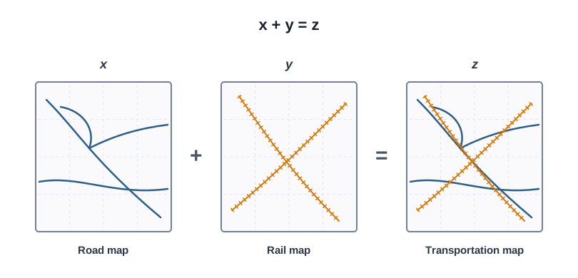
Fig. 4.10 – A simple spatial overlay operation.
Overlay has many uses. One of the most powerful is watching land use and land cover change between two dates, and reading the transformation that has taken place.
None of these three results existed as data before the overlay; each is new information pressed out of two ordinary land-use maps. That is what overlay does — it turns two snapshots into a record of change. And a record of change is exactly what a planner needs to see where a city is eating into its farmland, and to judge what the next stretch of land should become.
Map
Fig. 4.11 Caption: Urban land use in Aligarh city, Uttar Pradesh, in 1974 and 2001. Brief: Reproduce NCERT’s paired maps of Aligarh city, 1974 and 2001, side by side, with a north arrow and a scale bar reading up to 5,000 metres. Show the legend classes — residential, villages, commercial area, university area, grave yards, industrial area, fort, vacant land, tree plantation, agricultural land, water bodies/logged — and label the framing features (railway lines to Delhi, Bareilly and Kanpur, Grand Trunk Road, Ramghat Road, Agra Road, Aligarh Drain). Note the sources: Aligarh City Guide Map (1974) and IRS-1D panchromatic satellite imagery (2001).
Map
Fig. 4.12 Caption: Urban land transformations in Aligarh city, 1974–2001. Brief: Reproduce NCERT’s transformation map of Aligarh city with a north arrow and a scale bar to 5,000 metres. The legend must show each change class — no change, agriculture to residential, agriculture to vacant, agriculture to commercial, agriculture to industrial, residential to commercial, vacant to residential, vacant to industrial, village to residential — and the framing roads and railway lines as in Fig. 4.11.
Map
Fig. 4.13 Caption: Urban sprawl of Aligarh city, Uttar Pradesh, 1974–2001. Brief: Reproduce NCERT’s sprawl map of Aligarh city with a north arrow and a scale bar to 5,000 metres. The legend must distinguish the fort, the urban area of 1974, the urban area of 2001, non-urban land and water bodies, so the outward growth of the built-up area between the two dates is visible. Note the sources: Aligarh City Guide Map (1974) and IRS-1D satellite imagery (2001).
4.6.5.2 Buffer Operation
A buffer is a zone of a stated distance drawn around any point, line or area feature (Fig. 4.14). Buffers are used to find the people or places served by a facility — or denied it — whether a hospital, a medical store, a post office, a surfaced road or a park. They also measure who is exposed to a hazard: the households within a one-kilometre buffer of a chemical plant are the ones its waste can reach. This kind of study, of who lies near enough to be reached or affected, is called proximity analysis, and the buffer draws it as a polygon around the feature whatever that feature’s shape.
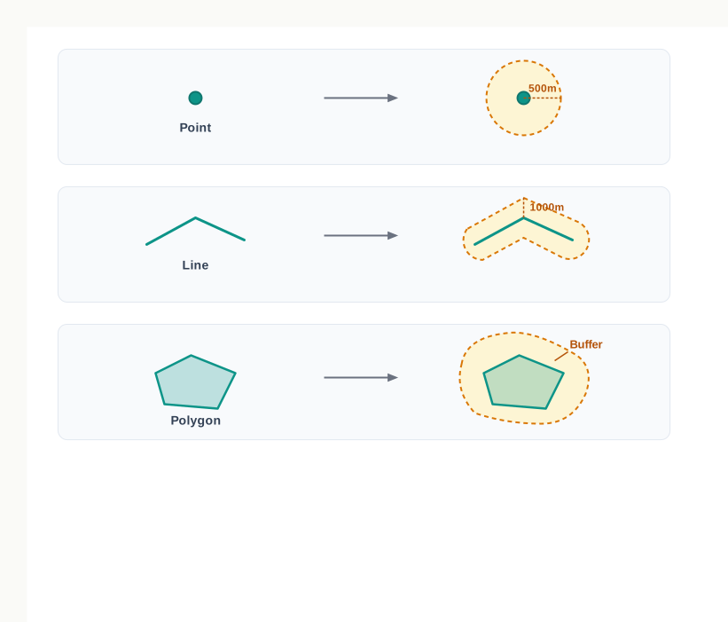
Fig. 4.14 – Buffers around point, line and polygon features.
GIS packages such as ArcView, ArcGIS, Geomedia and the free Quantum GIS all provide buffer tools for points, lines and areas. With them one can, for instance, draw buffers of 2, 4, 6, 8 and 10 kilometres around every city that has a major hospital, and so map how far its care reaches.
The buffers turn a vague sense of ‘distance to a hospital’ into something you can see and count. Land near the cities falls inside the inner rings and is well served; land far from every city lies beyond even the ten-kilometre ring and is the least benefitted, its people forced to travel long distances for care. Read this way, the map does more than describe the present — it points to where a new hospital would do the most good.
Map
Fig. 4.15 Caption: Location of the cities of western Uttar Pradesh. Brief: Reproduce NCERT’s location map showing the district outlines of western Uttar Pradesh with the six cities — Saharanpur, Muzaffarnagar, Meerut, Ghaziabad, Gautam Budh Nagar and Aligarh — marked as points in their correct relative positions.
Map
Fig. 4.16 Caption: Buffers of specified distances around city hospitals. Brief: Reproduce NCERT’s buffer map, showing the same western Uttar Pradesh outline with concentric buffer rings around each city hospital. The legend must key the ring distances — 2, 4, 6, 8 and 10 kilometres — so the reader can see how the served area widens ring by ring and where rings overlap between neighbouring cities.
To explore these tools further, NCERT points readers to three Indian resources on the web — schoolgis.nic.in, bhuvan.nrsc.gov.in and www.iirs.gov.in — where the ideas of this chapter can be seen at work on real data.
4.7 Summary
- Computers made two things possible early on — the Database Management System, for processing data, and Computer Assisted Cartography, for drawing maps — but neither could turn its output into a decision support system.
- Everyday questions about place, such as what is where, why it is there, what happens if it moves, and who gains or loses by the move, need data from many sources brought together under geo-processing tools. That is a Spatial Information System.
- Spatial means distributed over a definable space with measurable dimensions. Spatial Information Technology collects, stores, retrieves, displays, manipulates, manages and analyses such information, joining Remote Sensing, GPS, GIS, Digital Cartography and Database Management Systems.
- A GIS captures, stores, checks, integrates, manipulates, analyses and displays data that are spatially referenced to the Earth, working through a spatially referenced database and its application software.
- Geographical information comes in two forms — spatial data, which fixes location and appears as positional, linear and areal features, and non-spatial or attribute data, which describes those features.
- Spatial data for a GIS can be bought digitally, digitised from analogue records, or surveyed afresh. The choice depends on the application, the budget and the data structure needed.
- A paper map is limited: it presents information in one fixed way, carries only its predetermined themes, and must be redrawn to be changed. A GIS separates storage from display, so features can be interrogated, maps drawn by querying attributes, overlay and buffering applied, and attributes linked through a shared location code.
- Five components make a GIS — hardware, software, data, people and procedures.
- Raster format stores a feature as a grid of valued cells; resolution is the relationship between cell size and number of cells. It suits satellite images, scanned maps, low-cost work and backdrops.
- Vector format stores features as coordinate points joined into lines and polygons, and can carry topology. It suits precise applications, small files, analysis of individual features and stored descriptions.
- Each format is strong where the other is weak: raster overlays easily and handles satellite imagery but wastes storage and distorts shape; vector is compact and accurate but overlays with difficulty and cannot take satellite imagery.
- GIS work follows five activities in order — spatial data input, entering the attribute data, verification and editing, linking spatial to attribute data, and spatial analysis.
- Data bought from suppliers must be checked for compatibility of projection, scale, base level and attribute description, and trouble is worst where a study crosses administrative boundaries.
- Manual input runs through digitisation and scanning; scanners convert analogue maps into raster images, and every scan carries the original’s defects, which must be cleaned out.
- Captured data are verified against the original on a light table. Errors are of three kinds — data incomplete or doubled, data at the wrong scale, and data distorted — and editing them can take longer than the input itself.
- Layers used together must share one format, and conversion usually runs from vector to raster because most analysis is done there.
- Spatial and attribute data are joined by linkage and by matching — exact matching on a shared key, hierarchical matching where small areas nest inside large ones, and fuzzy matching where boundaries do not agree.
- Analysis is what sets a GIS apart. Overlay stacks thematic layers of the same area to yield a new layer, as with Aligarh’s land use, land transformation and urban sprawl. Buffering draws a zone of stated distance around a feature to measure proximity, as with the hospital buffers of western Uttar Pradesh.
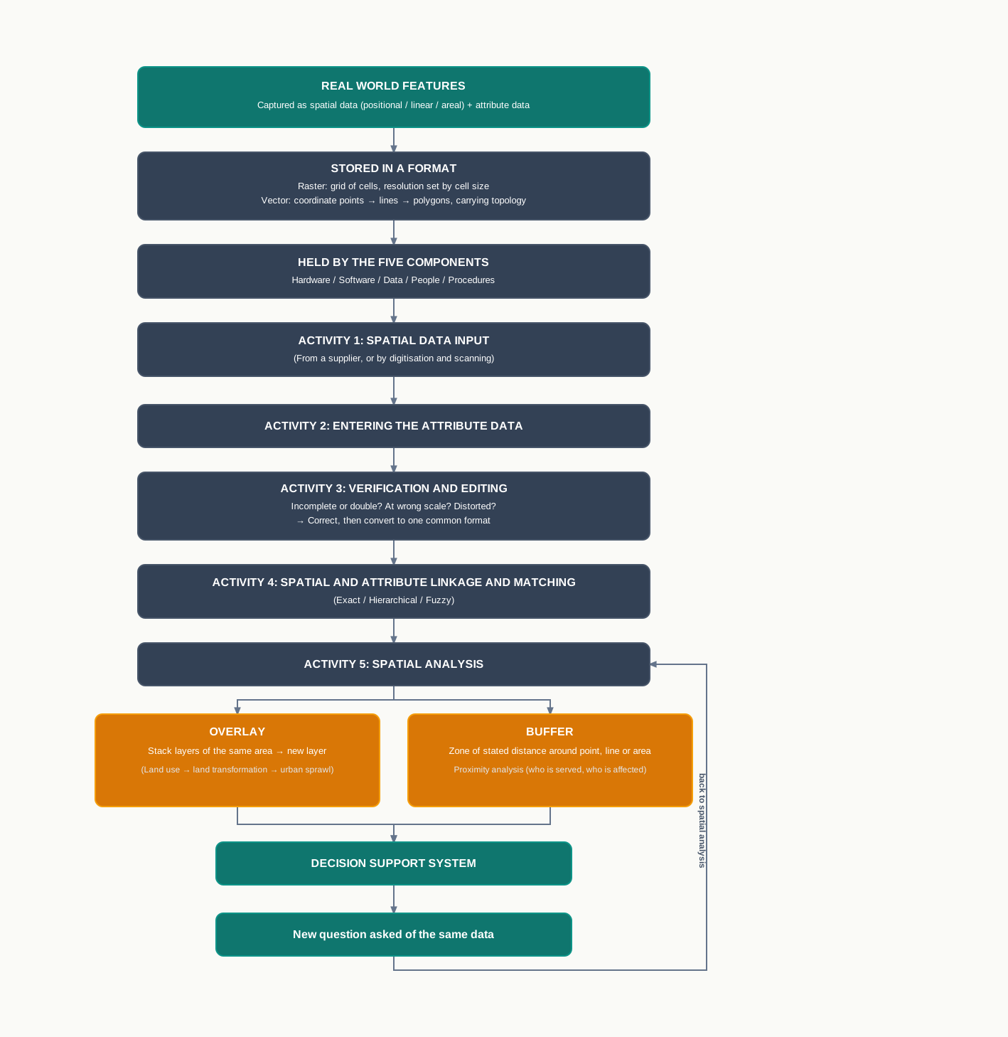
Fig. 4.17 – The complete GIS workflow.
What This Chapter Cannot Tell You
A GIS answers only as well as the data it was given. Every projection mismatch, wrong scale, distorted base map and uncorrected digitising error survives inside the system and comes out looking exactly as authoritative as good data — the screen shows no difference between the two.
The chapter’s own examples carry limits of scale and date. Aligarh’s maps compare two years, 1974 and 2001, so they record what changed across that gap but not when within it, nor why. The hospital buffers measure distance in a straight line from a city point; they say nothing about the roads a patient must actually travel, what the hospital can treat, or whether a household can afford to reach it.
And a decision support system supports a decision without making it. A buffer can show which areas are least benefitted; it cannot say whose need should be met first. That judgement stays with people, and the data only makes it better informed.
4.8 NCERT Questions
- The spatial data are characterised by the following forms of appearance:
- Positional
- Linear
- Areal
- All the above forms
- Which one of the following operations requires analysis module software?
- Data storage
- Data display
- Data output
- Buffering
- Which one of the following is disadvantage of Raster data format?
- Simple data structure
- Easy and efficient overlaying
- Compatible with remote sensing imagery
- Difficult network analysis
- Which one of the following is an advantage of Vector data format?
- Complex data structure
- Difficult overlay operations
- Lack of compatibility with remote sensing data
- Compact data structure
- Urban change detection is effectively undertaken in GIS core using:
- Overlay operations
- Proximity analysis
- Network analysis
- Buffering
Differentiate between raster and vector data models. (in about 30 words)
What is an overlay analysis? (in about 30 words)
What are the advantages of GIS over manual methods? (in about 30 words)
What are important components of GIS? (in about 30 words)
What are different ways in which spatial data is built in GIS core? (in about 30 words)
What is Spatial Information Technology? (in about 30 words)
Discuss raster and vector data formats. Give example. (in about 125 words)
Write an explanatory account of the sequence of activities involved in GIS related work. (in about 125 words)
4.9 Check Your Concepts
Look at the two records in Table 4.1 and Table 4.2. One of them can be used in a GIS and the other cannot. Say which is which, and identify the exact feature of the record that decides it.
Study Fig. 4.2. For each of the three features shown — the benchmark, the river and the lake — name its form of appearance, and suggest one item of attribute data a GIS might store alongside it.
Fig. 4.6 stores the same shape at two cell sizes. Show the arithmetic that gives each pixel count from its number of columns and rows, and state what the reader gains and what is paid for by moving from the coarser grid to the finer one.
The chapter says that most analysis is done in the raster domain, and that layers used together must all be in one format. Using the advantages and disadvantages of the two formats, explain why the usual conversion runs from vector to raster rather than the other way.
Set the sequence of GIS activities out in order, and explain what would go wrong at the analysis stage if the verification and editing stage were skipped. Draw on the three kinds of error the chapter names.
Exact matching, hierarchical matching and fuzzy matching all bring two sets of data together. Explain what makes each necessary, using the chapter’s own situations — towns in two files, land-use and land-transformation data, and crop boundaries against soil boundaries.
Fig. 4.16 shows buffers of 2, 4, 6, 8 and 10 kilometres around the city hospitals of western Uttar Pradesh. Explain how this map identifies the least benefitted areas, and then state two things about a household’s real access to hospital care that these buffers cannot tell you.