Chapter 4: Map Projections
Pull up almost any world map on a classroom wall and look at the far north. Greenland sits there as a vast white slab, apparently as wide as a whole continent, rivalling the great landmasses to its south. Then check an atlas that measures area honestly, and the illusion collapses. Greenland is a fraction of the size it appears. The map has stretched it out of all proportion.
This is not a printing mistake. It is the unavoidable cost of a single, stubborn problem. The Earth is a rounded body, close to a sphere, and its surface cannot be peeled off and laid flat without tearing, stretching or crushing some part of it. An orange peel will not lie flat on a table unless you split it and force it down. The globe behaves the same way.
Yet we cannot carry a globe into the field, pin it to a wall, or measure a road on it. We need flat maps. So cartographers accept a bargain: to gain a flat sheet, they must surrender something — true shape, true size, true direction or true distance. The whole craft of map projection is the art of choosing which of these to keep and which to let go, and knowing exactly what has been sacrificed.
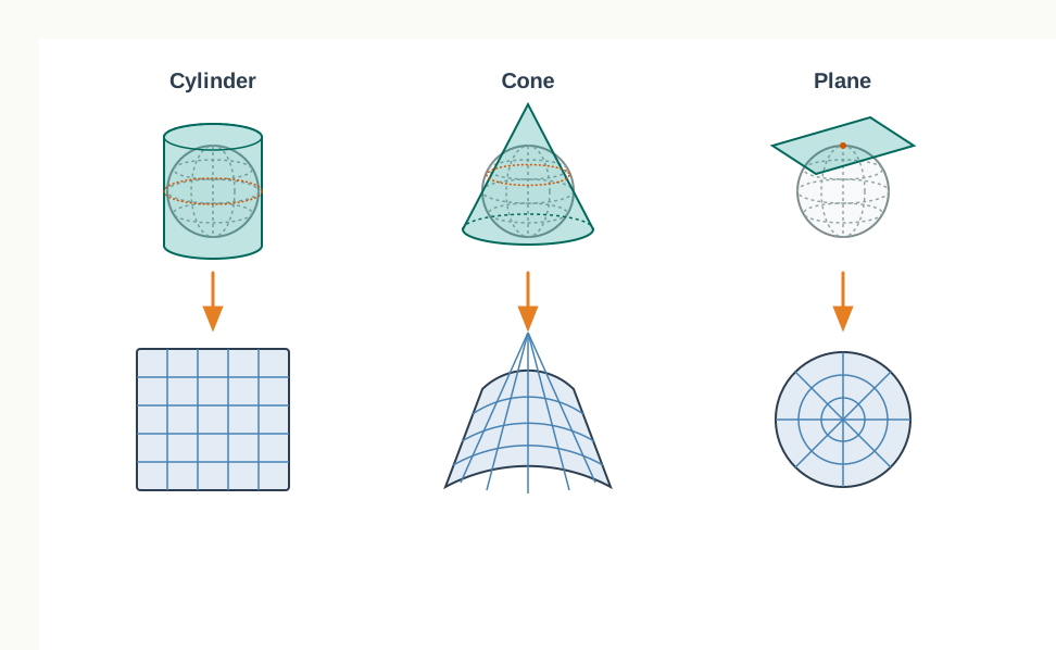
Fig. 4.0 – Developable surfaces: cylinder, cone and plane.
4.1 Map Projection
This chapter sets out to answer a few plain but essential questions. What is a map projection? Why do we draw one at all? What different types exist, and which type suits which part of the world? To reach those answers, we must first be clear about what a projection is and why we cannot do without it.
From A Round Earth To A Flat Sheet
Map projection is the method of transferring the graticule of latitude and longitude onto a plane surface. Put another way, it is the transformation of the spherical network of parallels and meridians onto a flat surface. That single sentence hides the whole difficulty of the subject, so it is worth unpacking slowly.
The Earth on which we live is not flat. It is geoid in shape — a rounded, very nearly spherical body (the word simply means ‘Earth-shaped’). Because of this, a globe, a small spherical model of the Earth, is the best model we have. On a globe the shapes and sizes of the continents and oceans are shown accurately, and directions and distances between places are also true.
A globe is ruled by two sets of lines. The horizontal lines running around it are the parallels of latitude, the circles that measure how far north or south a place lies. The vertical lines running from pole to pole are the meridians of longitude, which measure how far east or west it lies. Together this criss-cross of parallels and meridians is called the graticule, and it is this grid that makes map-drawing possible. Drawing that graticule on a flat surface is what we call projection.
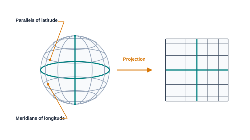
Fig. 4.1 – The globe’s graticule and its flat projection.
Why Not Simply Use The Globe?
If a globe shows everything so faithfully, why bother with flat maps at all? Because a globe has real limitations. It is expensive to make. It cannot be carried about easily or pinned to a wall, and it is too small to show the minor detail of any one region.
There is also a deeper, geometric problem. On the globe the meridians are semi-circles and the parallels are full circles, each curving in three dimensions. The moment we try to lay them out on a plane surface, they can no longer stay as they were: they become intersecting straight lines or curved lines instead. The contrast, then, is sharp. The globe is faithful but impractical; the flat map is practical but, as we shall see, never wholly faithful. Every projection is an attempt to get the best flat map we can out of that trade.
4.2 Need For Map Projection
Why A Globe Is Not Enough
The need for a map projection arises, above all, from the wish to study a region in detail — something a globe simply cannot do. A globe is too small and too general. It is also awkward for comparison: setting two natural regions side by side and measuring one against the other is not easy on a curved surface. What we usually want instead are accurate, large-scale maps on flat paper — a large-scale map being one that shows a small area in great detail.
That leaves one hard problem. How do we transfer the lines of latitude and longitude from a rounded globe onto a flat sheet? If we press a flat paper against the globe, the two will touch cleanly only at a point or along a line. Over any larger surface the paper cannot coincide with the globe without being distorted.
Where The Distortion Comes From
We can see the distortion appear if we imagine a light thrown from the centre of the globe. The shadow of the graticule falls onto the paper, but the picture it casts is distorted wherever the paper lies away from the line or point at which it touches the globe. The tangential point is exactly that point of contact — the one place where paper and globe meet. As we move outward from it, the rays strike the paper at an ever-shallower angle, and the distortion grows.
This is why tracing every property of the globe — its true shape, its true size, its true directions — onto flat paper is nearly impossible. The reason is fundamental: the globe is not a developable surface, meaning its curved skin cannot be unrolled flat without being stretched, torn or crushed.
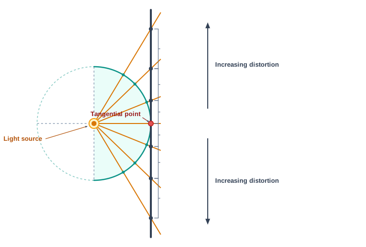
Fig. 4.2 – Distortion of the graticule cast from a central light source.
Living With Distortion
In a map projection we try to represent a good model of some part of the Earth in its true shape and dimension. Yet distortion in one form or another is inevitable — it can never be removed completely, only pushed around and controlled. To keep it in check, cartographers have devised many methods, and so many types of projection have come to be drawn.
For this reason, map projection is also defined in a second way: as the study of the different methods that have been tried for transferring the lines of the graticule from the globe to a flat sheet of paper. Each method is one more answer to the same stubborn question — how to flatten the round Earth while giving up as little of the truth as possible.
4.3 Elements Of Map Projection
Every projection is built from a few basic elements. Before we can draw one, we need to be clear about what a reduced model of the Earth is, what the parallels and meridians actually are, and which properties of the Earth’s surface a projection sets out to preserve.
4.3.1 Reduced Earth
A projection begins with a scaled-down stand-in for the planet. A model of the Earth is drawn to a reduced scale on a flat sheet of paper, and this model is called the reduced earth. It should be more or less spheroid — that is, very nearly spherical but slightly flattened, with its polar diameter a little shorter than its equatorial diameter. It is onto this reduced earth that the network of the graticule is transferred.
4.3.2 Parallels Of Latitude
The parallels of latitude are the circles running round the globe parallel to the equator, each keeping a uniform distance from the poles. Every parallel lies wholly within its own flat plane, and that plane sits at a right angle to the axis of the Earth — the imaginary line about which the Earth spins.
These circles are not all of equal length. They range from a full circle at the equator, matching the whole circumference of the globe, down to a mere point at each pole, where the parallel shrinks to nothing. They are numbered from 0° at the equator to 90° North and 90° South at the poles.
4.3.3 Meridians Of Longitude
The meridians of longitude are semi-circles drawn in the north–south direction, each running from one pole to the other. Two opposite meridians together make a complete circle equal to the circumference of the globe. Every meridian lies wholly within its own plane, and all of them intersect one another at a right angle along the Earth’s axis, where they meet at the poles.
Unlike the parallels, no meridian stands out naturally as the central one. So an arbitrary choice is made for convenience: the meridian passing through Greenwich, a place near London in England, is fixed as 0° longitude. It serves as the reference from which all other longitudes are drawn.
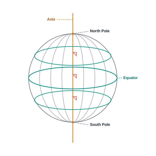
Fig. 4.3 – Parallels of latitude and meridians of longitude.
The Two Sets Of Lines Compared
It helps to hold the two apart clearly, because they behave very differently. The parallels are complete circles, all parallel to one another, but of unequal length — widest at the equator and shrinking to a point at each pole. The meridians are semi-circles, all of the same length, since each runs the full span from pole to pole. The parallels never meet; the meridians all converge and meet at both poles. And where they cross, they always do so at right angles. What they share is simple: together they form the graticule, the grid on which every map is built.
4.3.4 Global Property
When we prepare a map projection, there are four basic properties of the global surface that we try to preserve, using one method or another. This set of four is what we call the global property of a projection:
- the distance between any two given points of a region;
- the shape of the region;
- the size or area of the region, kept accurate;
- the direction, or bearing, of one point of the region towards another.
No single method can hold on to all four at once, as the next section will make clear. Which of them a projection keeps, and which it gives up, is the choice that defines it.
4.4 Classification Of Map Projections
Map projections may be classified on four different bases. The first looks at the method of construction. The second looks at the kind of surface the graticule is projected onto. The third asks which global property the map keeps true. The fourth asks where the source of light is placed. The same projection can therefore be described in several ways at once.
4.4.1 Drawing Techniques
On the basis of the method of construction, projections are generally sorted into three kinds: perspective, non-perspective, and conventional or mathematical.
A perspective projection is drawn with the help of a source of light, which projects the image of the network of parallels and meridians of a globe onto a developable surface. A non-perspective projection is developed without any source of light and without casting a shadow, on surfaces that can then be flattened. A mathematical or conventional projection is one worked out by mathematical computation and formulae; it has little relation to any actual projected image of light and shadow.
4.4.2 Developable Surface
Developable And Non-developable
The heart of this classification is a single idea. A developable surface is one that can be flattened, and onto which a network of latitude and longitude can be projected. A non-developable surface is one that cannot be flattened without shrinking, breaking or creasing.
A globe, or any spherical surface, is non-developable — this is the very difficulty the whole chapter turns on. But a cylinder, a cone and a plane are all developable: each can be unrolled or laid out flat. On the basis of which of these surfaces is used, projections are classified as cylindrical, conical and zenithal. When we try to flatten the globe directly, gaps open up between the strips of its surface, as the figure below shows.
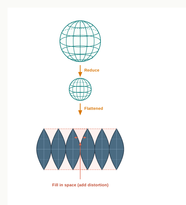
Fig. 4.4 – Flattening a globe produces gaps and distortion.
The Three Kinds Of Surface
Cylindrical projections are made using a cylindrical developable surface. A paper cylinder is wrapped around the globe, the parallels and meridians are projected onto it, and when the cylinder is cut open it gives a cylindrical projection on a flat sheet.
A conical projection is drawn by wrapping a cone round the globe, so that the shadow of the graticule network falls on it. When the cone is cut open, the projection is obtained on a flat sheet.
A zenithal projection (the word comes from zenith, the point directly overhead) is obtained directly on a plane surface. The plane touches the globe at a single point, and the graticule is projected onto it. Usually the plane is placed so that it touches the globe at one of the poles.
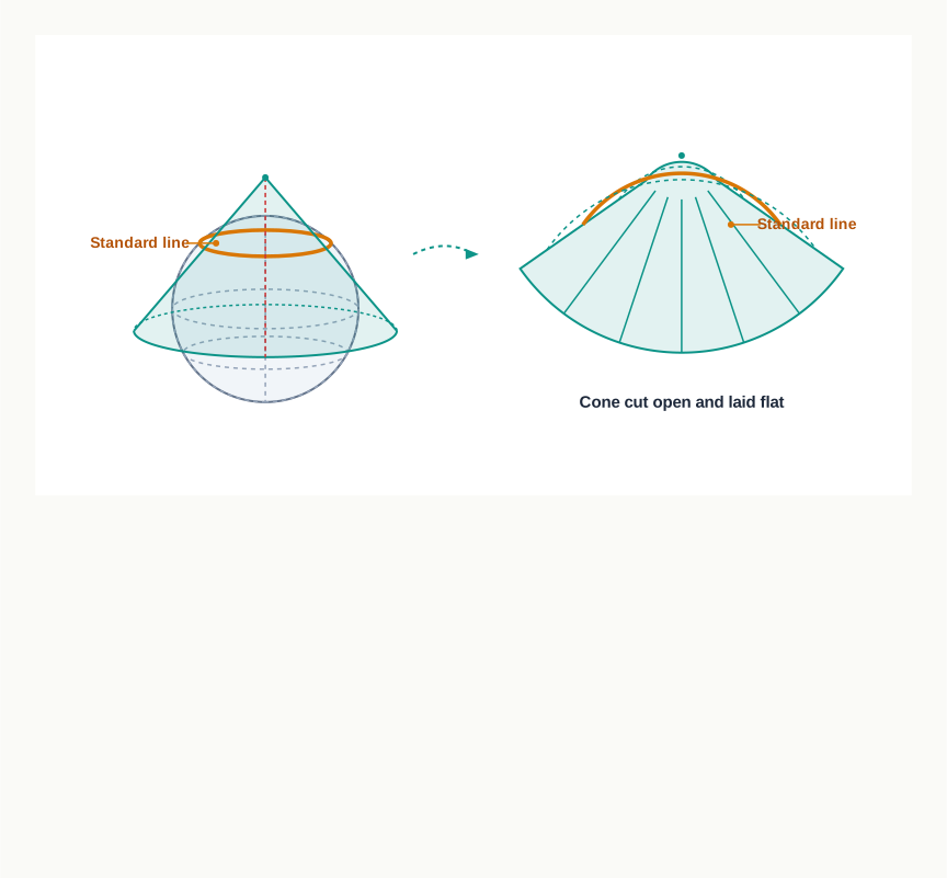
Fig. 4.5 – Conical projection from a globe to a flat sheet.
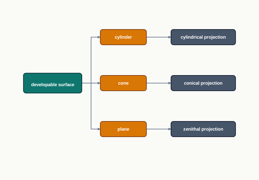
Fig. 4.6 – Classification of projections by developable surface.
Where The Surface Touches The Globe
These projections are subdivided again by the position at which the developable surface touches the globe. If it touches at the equator, the result is called the equatorial or normal projection. If it is tangential to a point between the pole and the equator, it is the oblique projection. And if it is tangential to the pole itself, it is the polar projection.
4.4.3 Global Properties
As we saw among the elements of projection, four global properties may be preserved in a map: the correctness of area, of shape, of direction and of distance. But none of the projections can hold on to all four at the same time. So, according to the specific need, a projection is drawn to keep whichever quality matters most for the job.
On this basis, projections are classified into four kinds. An equal area projection, also called the homolographic projection, is one in which the areas of various parts of the Earth are shown correctly. An orthomorphic or true-shape projection is one in which the shapes of areas are drawn correctly — and here the shape is generally kept at the cost of area, so the two cannot both be right. An azimuthal or true-bearing projection is one on which the direction of all points from the centre is shown correctly. An equi-distant or true scale projection is one where distance, or scale, is kept correct.
There is a catch with the last of these. No projection keeps the scale correct everywhere on the map. Scale can be held true only along some selected parallels and meridians, chosen as the requirement demands.
4.4.4 Source Of Light
The last basis of classification is the position of the source of light used to cast the graticule. On this basis, projections are gnomonic, stereographic or orthographic.
A gnomonic projection is obtained by putting the light at the centre of the globe. A stereographic projection is drawn when the source of light is placed at the periphery of the globe, at the point diametrically opposite the point at which the plane surface touches it. An orthographic projection is drawn when the source of light is placed at infinity from the globe — so far away that its rays arrive parallel — opposite the point at which the plane surface touches the globe.
4.5 Constructing Some Selected Projections
We now move from theory to the drawing board. Three projections are worked through here in full — a conical projection, a cylindrical equal area projection and Mercator’s projection. For each, we set a construction problem, work out the few measurements it needs, list the steps, and then weigh what the finished map does well and where it fails.
4.5.1 Conical Projection With One Standard Parallel
What The Projection Is
A conical projection is drawn by projecting the image of the graticule of a globe onto a developable cone that rests on the globe. The cone touches the globe along one parallel of latitude, and this parallel is called the standard parallel — the single line along which the map’s scale stays true. As the cone touches the globe along the line AB, the parallel where globe and cone coincide is taken as the standard parallel. The other parallels, on either side of it, are stretched out of their true length.
Working Out The Measurements
Before drawing, we settle three things: the size of the reduced earth, which parallel is the standard parallel, and which meridian runs down the centre. The radius of the reduced earth comes from the map’s scale — the actual radius of the Earth, written in centimetres, divided by the scale denominator, which shrinks it to the size it takes on paper.
The choice of the standard parallel is the whole decision. Scale is exactly right along it and grows steadily wrong away from it, so 40° N — sitting in the middle of the 10° N to 70° N belt — keeps the worst distortion off either edge. The central meridian, 70° E, simply fixes the line the fan of the map is built around.
Drawing It Step By Step
The construction follows eight steps.
- Draw a circle, or a quadrant, of 2.56 cm radius. Mark the angle COE as the 10° interval, and the angles BOE and AOD as 40°, the standard parallel.
- Extend a tangent from B to P, and another from A to P, so that AP and BP form the two sides of the cone touching the globe and giving the standard parallel at 40° N.
- The arc distance CE stands for the interval between parallels. Draw a semi-circle using this arc distance.
- Draw X–Y as the perpendicular from OP to OB.
- On a separate line N–S, mark off the distance BP to represent the standard parallel. This line N–S becomes the central meridian.
- Draw the other parallels by stepping off the arc distance CE along the central meridian.
- Mark the distance XY along the standard parallel at 40° to place the other meridians.
- Join these points to the pole with straight lines to complete the meridians.
The finished graticule is shown below.
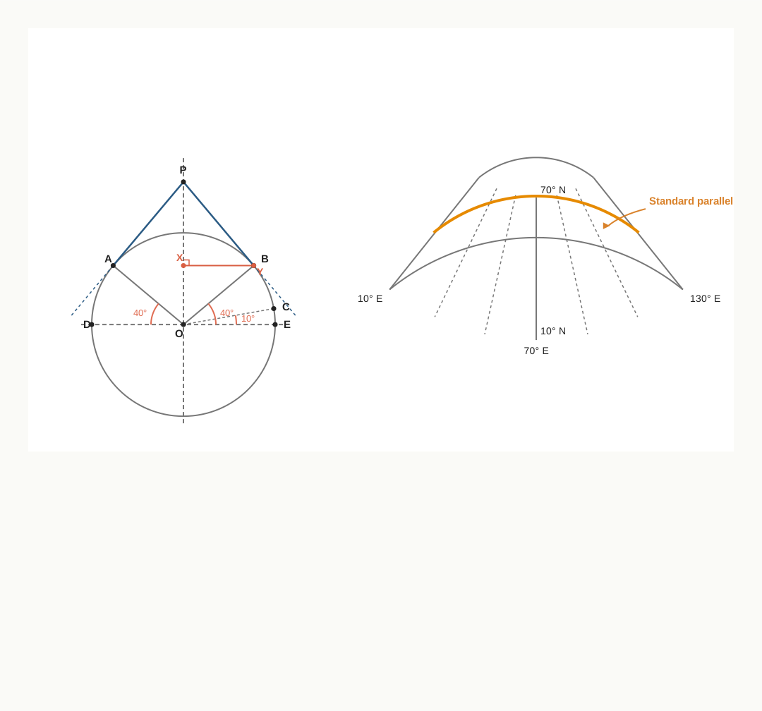
Fig. 4.7 – Simple conical projection with one standard parallel.
What It Keeps And What It Loses
This projection has a clear set of properties.
- All the parallels are arcs of concentric circles, equally spaced.
- All the meridians are straight lines meeting at the pole, and they cross the parallels at right angles.
- The scale along every meridian is true — distances measured along the meridians are accurate.
- An arc of a circle stands in for the pole.
- Scale is true along the standard parallel but exaggerated as we move away from it.
- The meridians draw closer together towards the pole.
- The projection is neither equal area nor orthomorphic.
Its limitations follow from that single true parallel:
- It is not suitable for a world map, because distortion becomes extreme in the hemisphere opposite the one holding the standard parallel.
- Even within one hemisphere it does not suit large areas, since distortion is greater near the pole and near the equator.
Its uses play to its one strength — a faithful east–west band:
- It is commonly used for mid-latitude areas that are limited in latitude but wide in longitude.
- A long narrow strip of land that runs parallel to the standard parallel, stretching east–west, is shown correctly.
- Direction along the standard parallel is reliable, so it is used to show railways, roads, narrow river valleys and international boundaries.
- It suits the Canadian Pacific Railways, the Trans-Siberian Railways (running east–west across Russia), the international boundary between the USA and Canada, and the Narmada valley in central India, which itself runs largely east–west.
4.5.2 Cylindrical Equal Area Projection
What The Projection Is
The cylindrical equal area projection, also called Lambert’s projection, is made by projecting the surface of the globe with parallel rays onto a cylinder that touches it at the equator. Both parallels and meridians come out as straight lines crossing one another at right angles. The pole is drawn as a line as long as the equator, and because of this the shape of the land is badly distorted at high latitudes — the price paid for keeping area correct.
Working Out The Measurements
Here we need the radius of the reduced earth, the length of the equator on the map, and the spacing of the meridians along it.
The interval works out this way because a full turn round the equator is 360°, so a 15° step is 15/360 of the whole equatorial line — and 15/360 of 13.2 cm is 0.55 cm. That single spacing, repeated, places every meridian.
Drawing It Step By Step
- Draw a circle of 2.1 cm radius.
- Mark the angles 15°, 30°, 45°, 60°, 75° and 90° for both the northern and southern hemispheres.
- Draw a line 13.2 cm long and divide it into 24 equal parts, each 0.55 cm apart. This line represents the equator. (It is 24 parts because 360° divided by the 15° interval gives 24.)
- Draw a line perpendicular to the equator at the point where 0° meets the circumference of the circle.
- Extend all the parallels from this perpendicular line, each made equal in length to the equator.
- Complete the projection as shown below.
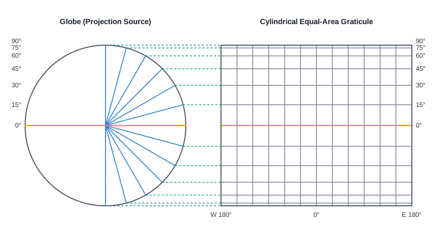
Fig. 4.8 – Cylindrical equal area projection for the world.
What It Keeps And What It Loses
Its properties are few and plain:
- All parallels and meridians are straight lines crossing each other at right angles.
- The polar parallel is as long as the equator.
- Scale is true only along the equator.
Its limitations are the cost of holding area equal:
- Distortion increases as we move towards the pole.
- The projection is non-orthomorphic — it does not keep true shape.
- Equality of area is kept at the cost of distortion in shape.
Because it shows area honestly, its uses are about area and distribution:
- It is most suitable for the belt lying between 45° N and 45° S.
- It is well suited to showing the distribution of tropical crops such as rice, tea, coffee, rubber and sugarcane.
That last use is worth pausing on. A distribution map is really an argument about how much land something covers, so it must show area truthfully. An equal area projection does exactly that, which is why the spread of a crop across the tropics is honestly compared on it — a region that grows twice as much appears twice as large, with no false stretching to mislead the eye.
4.5.3 Mercator’s Projection
What The Projection Is
A Dutch cartographer, Mercator Gerardus Karmer, developed this projection in 1569. It is built from mathematical formulae, and it is orthomorphic — the correct shape is kept. The distance between parallels increases towards the pole. As in the cylindrical projection, parallels and meridians cross at right angles. Its special virtue is that it shows correct directions: a straight line joining any two points gives a constant bearing, a fixed compass direction, and such a line is called a Laxodrome or Rhumb line.
Working Out The Measurements
This example is worked in inches rather than centimetres.
With the equator fixed at 6.28 inches and the meridians spaced every 0.26 inch, only one thing remains: how far up the map each parallel should sit. On Mercator’s projection this distance grows faster than the latitude itself, and it is read off from the chapter’s own table below.
The equator is divided into 24 equal parts, each part being the length of the equator times the interval, divided by 360. The distance of each parallel from the equator is then taken from the following table, in which each figure is multiplied by the reduced earth’s radius of 1 inch.
Read down the table and the point of the projection becomes visible: from the equator to 15° is only 0.265 inch, but from 60° to 75° the same 15° of latitude jumps by 0.71 inch. Equal steps of latitude are drawn further and further apart as we climb towards the pole — which is exactly how Mercator keeps shape correct.
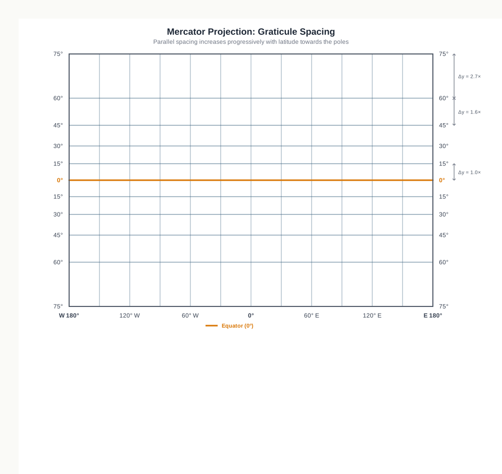
Fig. 4.9 – Mercator’s projection for the world.
What It Keeps And What It Loses
Its properties are the fullest of the three:
- All parallels and meridians are straight lines crossing at right angles.
- All parallels have the same length, equal to the length of the equator.
- All meridians have the same length and equal spacing, but each is longer than the matching meridian on the globe.
- The spacing between parallels increases towards the pole.
- Scale along the equator is correct, since it equals the equator on the globe. Other parallels are longer than the matching parallel on the globe, so scale is not correct along them — the 30° parallel, for instance, is 1.154 times longer than the corresponding parallel on the globe.
- Shape is maintained, but at higher latitudes distortion sets in.
- The shape of small countries near the equator is truly preserved, while distortion grows towards the poles.
- It is an azimuthal projection.
- It is orthomorphic, because the scale along the meridian equals the scale along the parallel.
Its limitations both come from that stretching:
- Scale is greatly exaggerated along parallels and meridians in high latitudes, so the size of countries near the pole is hugely overstated — the size of Greenland comes out equal to that of the USA, though it is really about one-tenth of the USA.
- The poles cannot be shown at all, because the 90° parallel and the meridians touching it become infinitely far apart.
Its uses rest on true direction and true shape near the equator:
- It is well suited to a world map and is widely used in preparing atlas maps.
- It is very useful for navigation, showing sea routes and air routes.
- Drainage patterns, ocean currents, temperature, winds and their directions, the spread of world rainfall and other weather elements are all shown appropriately on it.
We can see the difference between such a straight course and the true shortest route on the map itself.
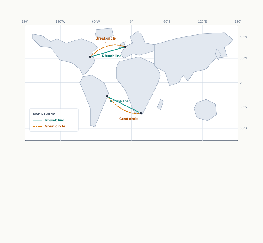
Fig. 4.10 – Rhumb lines and great circles on Mercator’s projection.
A rhumb line is easy to steer but longer; a great circle is the shortest path but keeps changing its bearing. On this one projection you can see both at once, which is a large part of why it has stayed the navigator’s map for so long.
4.6 Summary
- A map projection is a method of transferring the graticule — the network of parallels of latitude and meridians of longitude — from the round globe onto a flat surface.
- A globe shows shape, size, direction and distance faithfully, but it is expensive, cannot be carried about, and cannot show fine detail. For detailed, large-scale study, and for comparing regions, we need flat maps.
- The globe is a non-developable surface, so it cannot be flattened without stretching, tearing or crushing. Distortion is therefore inevitable; it grows with distance from the point of contact and can only be controlled, never removed.
- The elements of a projection are the reduced earth (a scaled-down model), the parallels of latitude (unequal circles, 0° to 90° north and south), the meridians of longitude (equal semi-circles meeting at the poles, with Greenwich fixed at 0°), and the four global properties a map tries to keep — distance, shape, size or area, and direction.
- Projections are classified on four bases: by drawing technique (perspective, non-perspective, mathematical or conventional); by developable surface (cylindrical, conical, zenithal — and, by where the surface touches, normal or equatorial, oblique, and polar); by global property (equal area or homolographic, orthomorphic or true-shape, azimuthal or true-bearing, equi-distant or true scale); and by source of light (gnomonic, stereographic, orthographic).
- No single projection can keep all four properties true at once, so each is chosen for the quality that matters most to the task.
- A conical projection with one standard parallel keeps scale true along the standard parallel but exaggerates it away from that line. It is neither equal area nor orthomorphic, and it suits long east–west strips in the mid-latitudes.
- A cylindrical equal area projection (Lambert’s) keeps area correct but distorts shape badly at high latitudes. It suits distribution maps of the belt between 45° N and 45° S.
- Mercator’s projection (1569) is orthomorphic and shows true direction: a straight line on it is a rhumb line of constant bearing. Its parallels spread further apart towards the poles, so size is hugely exaggerated there — Greenland comes out as large as the USA — and the poles cannot be shown at all. It remains the navigator’s map.
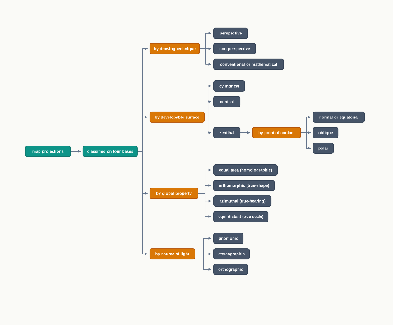
Fig. 4.11 – Classification of map projections on four bases.
What This Chapter Cannot Tell You
The chapter constructs only three projections out of the many that exist, and it does not name any one of them as the best — the best projection depends entirely on the purpose of the map. Each worked example is fixed to one scale and one interval, so its exact measurements belong to that example alone and change the moment the scale changes. And a flat line drawing cannot show the distortion it carries: an evenly ruled grid looks orderly on the page, so the stretching of area and shape has to be stated in words and figures, not seen directly in the map.
4.7 NCERT Questions
A map projection least suitable for the world map:
- Mercator
- Simple Cylindrical
- Conical
- All the above
A map projection that is neither the equal area nor the correct shape and even the directions are also incorrect:
- Simple Conical
- Polar zenithal
- Mercator
- Cylindrical
A map projection having correct direction and correct shape but area greatly exaggerated polewards is:
- Cylindrical Equal Area
- Mercator
- Conical
- All the above
When the source of light is placed at the centre of the globe, the resultant projection is called:
- Orthographic
- Stereographic
- Gnomonic
- All the above
Describe the elements of map projection.
What do you mean by global property?
Not a single map projection represents the globe truly. Why?
How is the area kept equal in cylindrical equal area projection?
Differentiate between
Developable and non-developable surfaces.
Homolographic and orthographic projections.
Normal and oblique projections.
Parallels of latitude and meridians of longitude.
Discuss the criteria used for classifying map projection and state the major characteristics of each type of projection.
Which map projection is very useful for navigational purposes? Explain the properties and limitations of this projection.
Discuss the main properties of conical projection with one standard parallel and describe its major limitations.
Construct graticule for an area stretching between 30° N to 70° N and 40° E to 30° W on a simple conical projection with one standard parallel with a scale of 1:200,000,000 and interval at 10° apart.
Prepare graticule for a Cylindrical Equal Area Projection for the world when R.F. is 1:150,000,000 and the interval is 15° apart.
Draw a Mercator Projection for the world map when the R.F. is 1:400,000,000 and the interval between the latitude and longitude is 20° apart.
4.8 Check Your Concepts
Look at Fig. 4.9 and Table 4.1. Is the north–south spacing greater between 0° and 15°, or between 60° and 75°? Give the two figures from the table, and explain what this widening spacing achieves for the shape of the land.
The radius of the reduced earth is found by dividing 640,000,000 by the scale denominator, which gives 2.1 cm at a scale of 1:300,000,000. Using the same method, work out the radius of the reduced earth at a scale of 1:250,000,000, and explain why a smaller scale denominator produces a larger reduced earth.
On the cylindrical equal area projection, the equator is 13.2 cm long and is divided using a 15° interval. Show, step by step, how the interval of 0.55 cm along the equator is obtained, and explain why the equator ends up divided into exactly 24 parts.
The chapter classifies projections by the position of the source of light. State where the light is placed in a gnomonic projection and where it is placed in an orthographic projection, and explain how this difference sets the two apart.
The chapter says the conical projection with one standard parallel suits the Trans-Siberian Railways and the Narmada valley. Using the projection’s properties, explain what these two have in common that makes this projection right for them.
A cylindrical equal area map shows the area of regions correctly but distorts their shapes at high latitudes. Explain why a geographer mapping the world distribution of a tropical crop would still choose this projection, despite that distortion of shape.