Chapter 6: Introduction To Remote Sensing
In June 2004, a satellite passed over the coast of Banda Aceh, on the northern tip of Sumatra in Indonesia, and recorded an ordinary scene: red-roofed houses packed along the shore, roads threading between them, boats resting at the water’s edge. The satellite never touched the town. It simply caught the sunlight reflected off roofs, water and trees and turned that light into numbers.
Six months later, in December 2004, a wave rose out of the Indian Ocean and struck that coast. The tsunami killed many people along the shoreline and swept whole neighbourhoods away in minutes.
When the satellite next passed over, it recorded the same patch of ground, now unrecognisable. Where streets and houses had stood, the image showed bare mud and open water. Nothing on the sensor had changed; only the surface below it had.
No survey team could have stood on that coast at that hour to measure the loss. Yet from hundreds of kilometres up, an instrument that touched nothing had recorded exactly what the wave had taken. That is remote sensing: learning about a place from a distance by reading the energy that leaves its surface. This chapter follows that energy from the Sun to the sensor and back to a finished map, and teaches you to read the images it makes along the way.
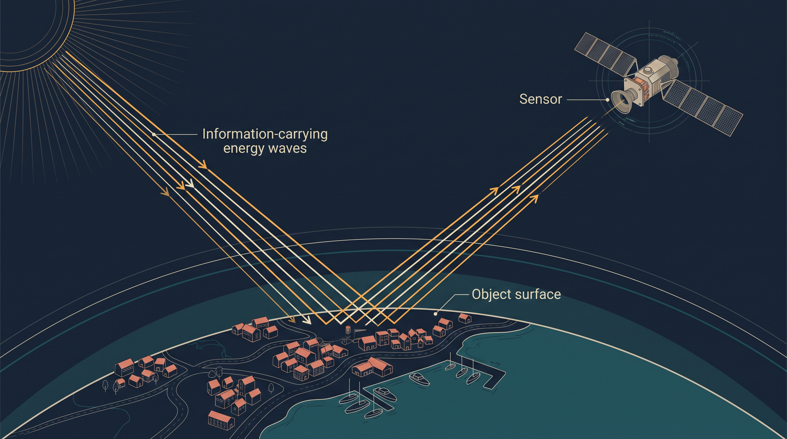
Fig. 6.0 – A satellite sensor reading a coastline from orbit.
6.1 What Remote Sensing Is
Look at anything around you — a wall, a leaf, the page of this book — and you can see it because light bounces off its surface into your eyes. But your eyes, like an ordinary photographic camera, respond to only a very small portion of the energy that surfaces give off. That portion is visible light. A great deal more energy is leaving every surface all the time, unseen by us.
Modern remote sensing devices react to a far wider range of radiation than the eye can. They respond to energy that surfaces reflect, emit, absorb and transmit. In fact, every surface warmer than 0 Kelvin gives off energy of some kind. Here 0 Kelvin, or −273°C, is absolute zero, the coldest temperature that can exist; nothing in the real world is ever that cold, so every real surface is constantly radiating energy that an instrument can read.
Sensing Without Touching
The term remote sensing was first used in the early 1960s. It was later defined as the whole set of processes used to acquire and measure information about some property of objects and phenomena, using a recording device — a sensor — that is not in physical contact with the objects and phenomena being studied.
The word remote is the heart of this definition. The sensor reads its target from a distance, touching nothing. It never lands on the field, dips into the river or walks the city street; it only receives the energy those surfaces send it.
The Three Essentials
From this definition, three things must always be present for remote sensing to happen (Fig. 6.1). There must be an object surface, whose properties we want to know. There must be a recording device, the sensor. And there must be information-carrying energy waves travelling between the two. It is these waves, and nothing else, that carry the object’s information across the gap to the sensor. Take away any one of the three and there is no remote sensing at all.
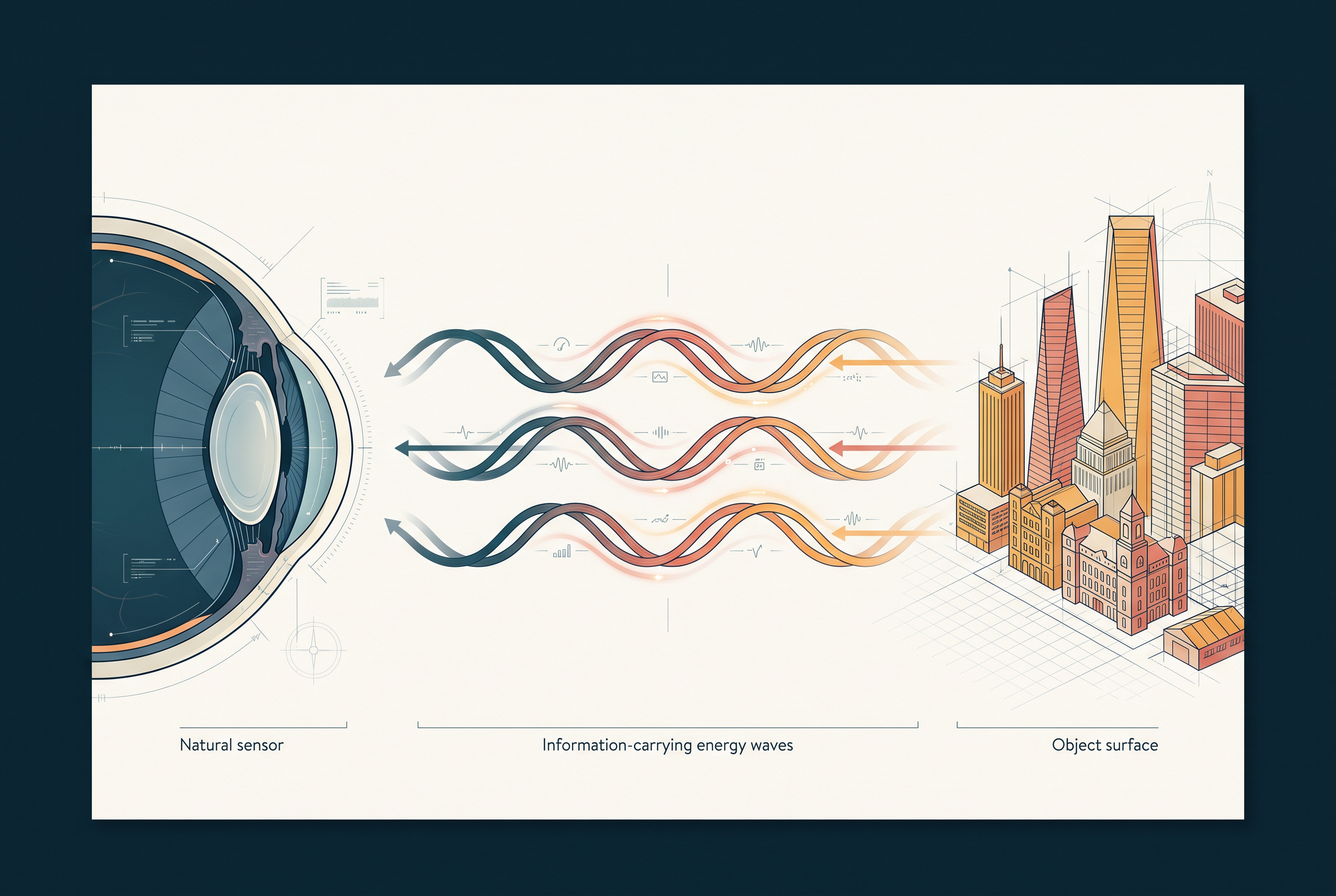
Fig. 6.1 – The three essentials of remote sensing.
Many of the terms this chapter uses again and again are gathered together for reference below, in the order the book lists them.
6.2 Stages In Remote Sensing
Remote sensing is not a single act but a chain of stages. Energy starts at a source, travels to the ground, bounces back, is caught by a sensor, and is finally turned into a map or a table you can read. Figure 6.2 lays out this whole sequence, and the same chain is set out step by step below.
The basic stages that together collect information about the objects and phenomena of the Earth’s surface are: the source of energy (the Sun, or self-emission); the transmission of energy from the source to the Earth’s surface; the interaction of that energy with the surface; the propagation of the reflected or emitted energy back through the atmosphere; the detection of that energy by the sensor; the conversion of the received energy into photographic or digital data; the extraction of information from those data products; and the conversion of that information into map or tabular forms.
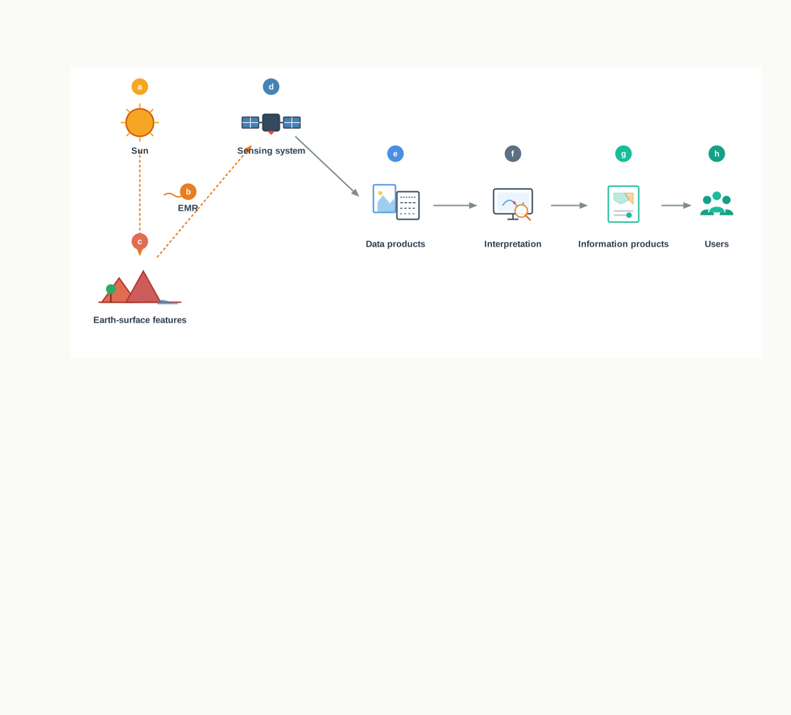
Fig. 6.2 – The stages of remote sensing data acquisition.
Because these stages follow one after another, they are easiest to hold in mind as a single flow.
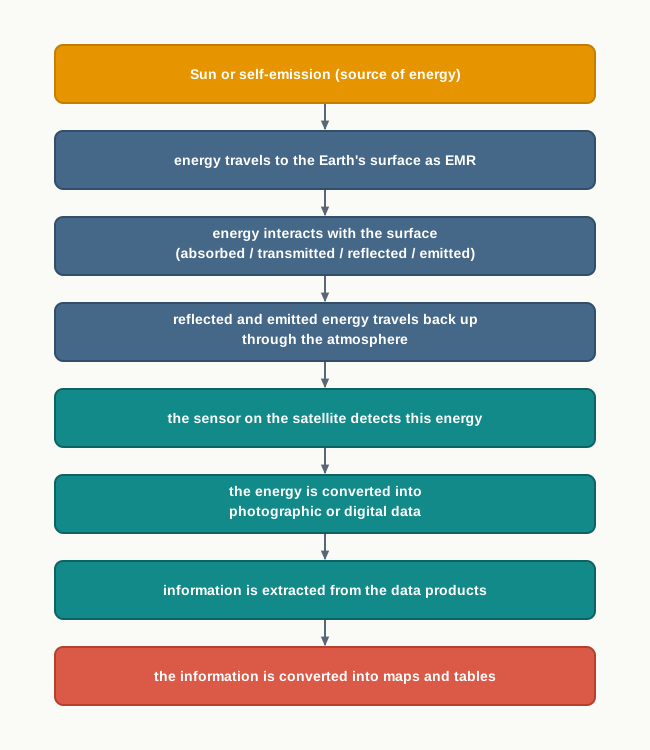
Fig. 6.3 – Remote sensing runs as a chain.
6.2.1 Source Of Energy
Every stage begins with energy, and the Sun is the most important source used in remote sensing. Sunlight falls on the Earth’s surface, and it is the sunlight bouncing back that most sensors read.
Energy can also be generated artificially and then used to collect information about objects and phenomena. Flashguns do this on a small scale. On a larger scale, radar — short for radio detection and ranging — sends out its own energy beam and reads what returns. The difference matters: a sensor relying on the Sun must wait for daylight and clear skies, while a system that makes its own energy can work in the dark and see through cloud.
6.2.2 Transmission Of Energy From The Source To The Surface Of The Earth
The energy that leaves a source travels to the object surface in the form of waves, moving at the speed of light — 300,000 km per second. This travelling energy is called Electromagnetic Radiation (EMR).
These energy waves vary in size and frequency. Plotting all those variations together gives the Electromagnetic Spectrum (Fig. 6.4). As a rule, the shorter the wave, the higher its frequency. On the basis of wave size and frequency, the energy is grouped into Gamma rays, X-rays, Ultraviolet rays, Visible rays, Infrared rays, Microwaves and Radio waves.
Each of these broad regions of the spectrum is used in different applications. Of them, it is the visible, infrared and microwave regions that are used in remote sensing.
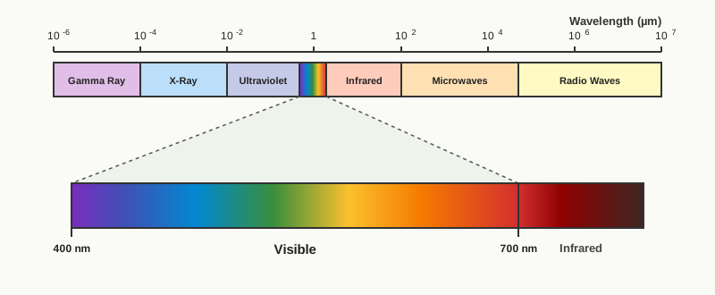
Fig. 6.4 – The electromagnetic spectrum.
6.2.3 Interaction Of Energy With The Earth’s Surface
The propagating energy finally meets the objects on the Earth’s surface. This meeting leads to the energy being absorbed, transmitted, reflected or emitted by those objects.
All objects differ in their composition, their appearance and their other properties, so no two objects respond to the energy they receive in exactly the same way. More than that, a single object responds differently in different regions of the spectrum (Fig. 6.6). This uneven response, spread across the wavelengths, is what lets a sensor tell surfaces apart.
Reading A Surface By Its Reflectance
The way a surface reflects energy across the wavelengths is its spectral signature, and Figure 6.5 shows the signatures of dry soil, vegetation and water side by side. Each surface has its own shape of curve, and it is this difference in shape that identifies it.
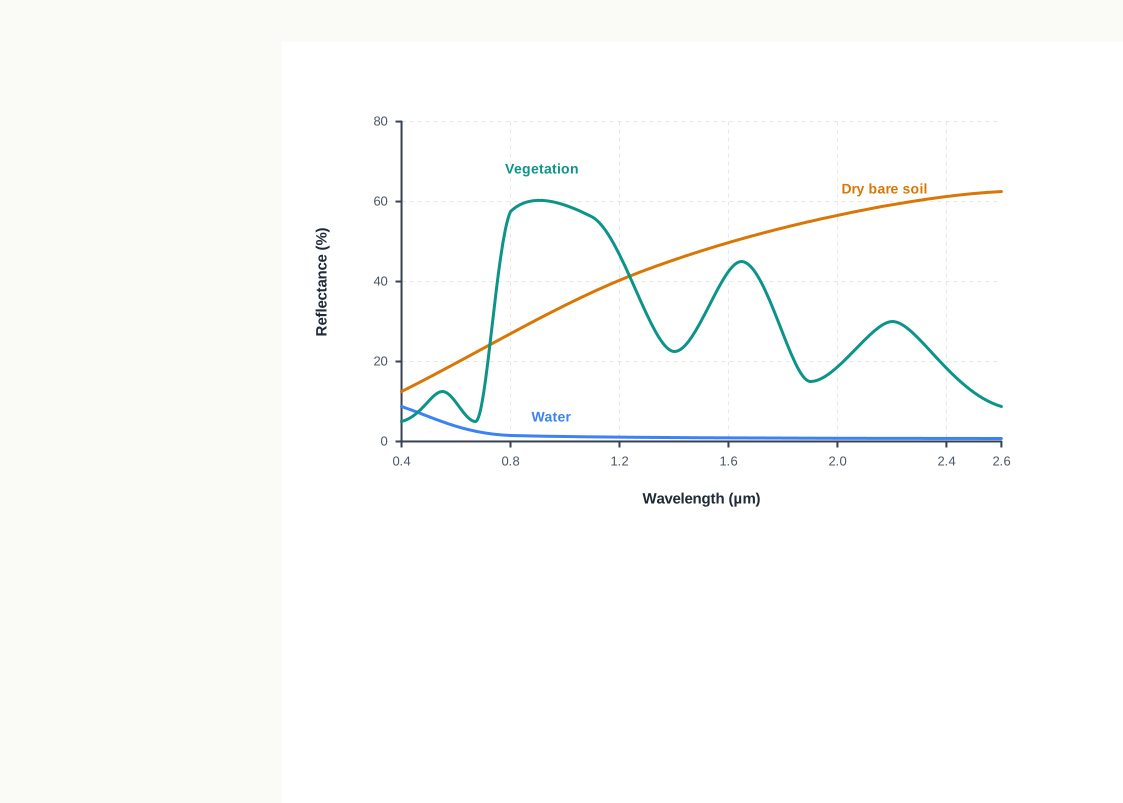
Fig. 6.5 – Spectral signatures of dry soil, vegetation and water.
Why Water Looks Dark
Take water as an example. A fresh water body absorbs much of the energy it receives in the red and infrared regions, so little energy returns to the sensor and the water appears dark, almost black, in a satellite image. A turbid, muddy water body behaves differently: the suspended particles reflect more energy in the blue and green regions, so it comes back in a lighter tone. The two images of Sambhar Lake — a large salt lake in Rajasthan, in western India — in Figure 6.6 show this difference between bands.
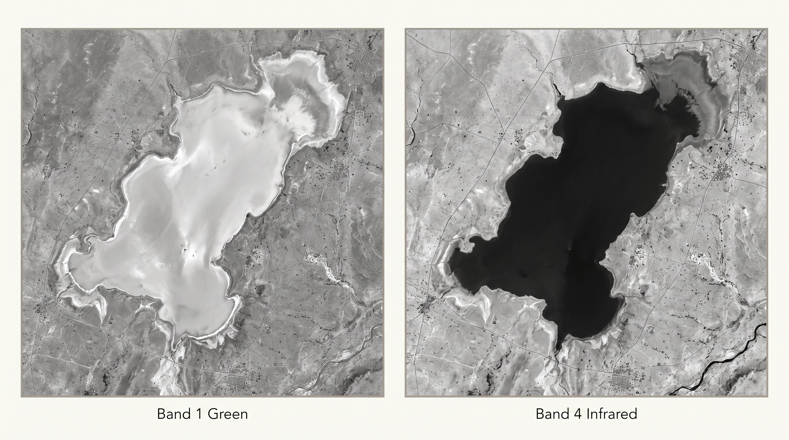
Fig. 6.6 – Sambhar Lake in green and infrared bands.
6.2.4 Propagation Of Reflected/Emitted Energy Through Atmosphere
When energy is reflected from the objects of the Earth’s surface, it re-enters the atmosphere on its way up to the sensor. The atmosphere is not empty: it is made of gases, water molecules and dust particles.
As the reflected energy passes through, it comes into contact with these constituents, and its original properties are changed. Carbon dioxide (CO₂), hydrogen (H) and water molecules absorb energy in the middle infrared region, while dust particles scatter the blue energy.
Energy that is absorbed or scattered in this way never reaches the sensor onboard the satellite. When that happens, the information about the objects carried by those energy waves is simply left unrecorded. This is one reason remote sensing works only in certain regions of the spectrum, where the atmosphere lets energy through.
6.2.5 Detection Of Reflected/Emitted Energy By The Sensor
The sensors that record the returning energy are carried on satellites, and where a satellite is placed decides what it can do. Remote sensing sensors sit in a near-polar sun-synchronous orbit at an altitude of 700 to 900 km. Satellites in this orbit are the remote sensing satellites, such as the Indian Remote Sensing (IRS) series.
Weather-monitoring and telecommunication satellites are placed very differently, in a geostationary position. Such a satellite is always held over the same part of its orbit, synchronised with the direction of the Earth’s rotation, so that it revolves along with the Earth’s spin and appears to stay above one place. It orbits at an altitude of nearly 36,000 km, far higher than a remote sensing satellite. The INSAT series is an example. Figure 6.7 shows the two kinds of orbit together.
Two Orbits Compared
The two families of satellite differ at almost every point. A sun-synchronous remote sensing satellite flies at 700 to 900 km, covers the globe from about 81°N to 81°S, completes about 14 orbits in a day, and returns a fine resolution of between 182 metre and 1 metre — which is why it is used for Earth resources applications. A geostationary satellite sits at about 36,000 km, sees roughly one-third of the globe at once, keeps step with the Earth over a 24-hour period, and returns only a coarse resolution of about 1 km by 1 km — which suits telecommunication and weather monitoring, where a wide, constant view matters more than fine detail.
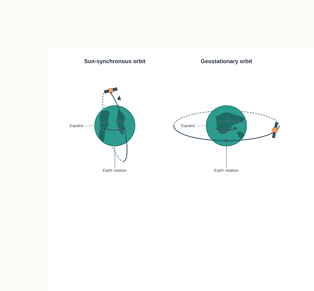
Fig. 6.7 – Sun-synchronous and geostationary orbits.
The remote sensing satellites are fitted with sensors able to collect the EMR reflected by the objects. A photographic camera captures a whole scene in a single instant of exposure. The sensors on remote sensing satellites work by a different mechanism when collecting and recording, and the images they produce are in digital format, unlike the photographic format of a camera-based system.
6.2.6 Conversion Of Energy Received Into Photographic/Digital Form Of Data
The radiations that reach the sensor are converted electronically into a digital image — a set of digital numbers arranged in rows and columns. These numbers can also be turned into an analogue, or picture, form of the data product.
The sensor onboard an Earth-orbiting satellite does not keep the data; it transmits the collected image data electronically to an Earth Receiving Station. Such stations are located in different parts of the world. In India, one such station is at Shadnagar, near Hyderabad in southern India.
6.2.7 Extraction Of Information Contents From Data Products
Once the image data reaches the earth station, it is first processed to remove the errors that crept in while the data was being collected. Only a corrected image is worth interpreting.
From the corrected image, the information is then drawn out. For digital images this is done using digital image processing techniques, run by computer. For analogue data products it is done by visual interpretation — a person reading the image by eye. The chapter returns to visual interpretation in detail later.
6.2.8 Conversion Of Information Into Map/Tabular Forms
The information that has been interpreted is finally shaped into something a reader can use. It is delineated and converted into separate layers of thematic maps, each map showing one kind of feature.
Alongside the maps, quantitative measures are taken from the data to build tabular data. With this last step the chain that began at the Sun ends where geography needs it — as maps and tables.
6.3 Sensors
A sensor was defined earlier as the recording device of remote sensing. More fully, it is a device that gathers electromagnetic radiation, converts it into a signal, and presents that signal in a form from which information about the objects under study can be drawn.
Sensors are classified by the form of data they output. A photographic, or analogue, sensor is one kind; a non-photographic, or digital, sensor is the other.
A photographic sensor is simply a camera. It records the images of objects at one instance of exposure, capturing the whole scene in a single moment. A non-photographic sensor works differently: it builds the image bit by bit. These bit-by-bit sensors are called scanners. The rest of this chapter deals only with the non-photographic scanners used in satellite remote sensing.
6.3.1 Multispectral Scanners
The scanners used in satellite remote sensing are the Multispectral Scanners (MSS). They are designed to build up an image of the objects while sweeping across the field of view.
A scanner is usually made of a reception system — a mirror and a set of detectors. It constructs the scene by recording one scan line after another. A motor swings the scanning mirror through the angular field of view of the sensor, and the reach of that swing sets the length of each scan line; this length is called the swath. Because the image is assembled one line, and within each line one cell, at a time, the scanner’s way of collecting an image is described as bit-by-bit.
Each scene is made of cells, and the size of these cells fixes the spatial resolution of the image — how much fine detail on the ground the image can keep apart. As the mirror oscillates across the scene, it directs the received energy onto the detectors, where the energy is turned into electrical signals. These signals are then converted into numerical values called the Digital Number (DN values), which are recorded for storage.
Multispectral Scanners are of two types — whiskbroom scanners and pushbroom scanners.
6.3.1.1 Whiskbroom Scanners
A whiskbroom scanner is made of a rotating mirror and a single detector. The mirror is set so that, as it completes a rotation, the single detector is swept across the field of view, between 90° and 120°. In that sweep it gathers images in a large number of narrow spectral bands, ranging from the visible to the middle infrared regions of the spectrum.
The full extent of this oscillating sweep is called the Total Field of View (TFOV) of the scanner. While it scans the whole field, the sensor’s optical head is always held at one particular dimension called the Instantaneous Field of View (IFOV) — the small patch it is looking at in any one instant. Figure 6.8 shows how a whiskbroom scanner works.
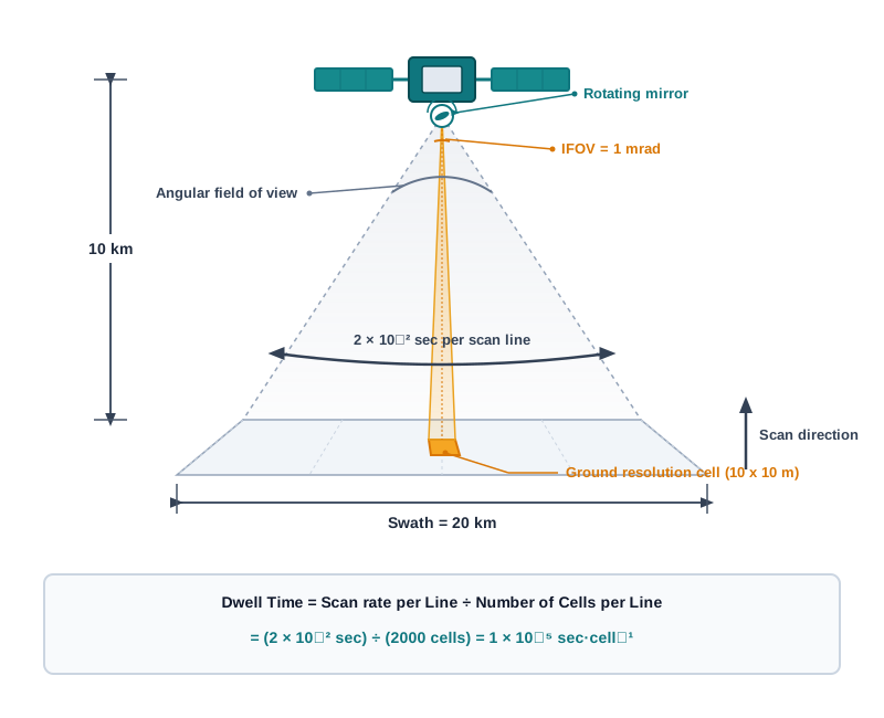
Fig. 6.8 – A whiskbroom scanner sweeping a single detector.
6.3.1.2 Pushbroom Scanners
A pushbroom scanner does away with the moving mirror. Instead it uses a row of detectors, and the number of detectors it needs is found by dividing the swath of the sensor by the size of the spatial resolution.
The chapter works this out for a real sensor: the High Resolution Visible Radiometer-1 (HRVR-1) carried by the French remote sensing satellite SPOT, whose swath is 60 km and whose spatial resolution is 20 metres.
Those 3000 detectors are linearly arrayed — lined up side by side in a single row. Each one is fixed on its own 20-metre-wide strip of ground directly below the satellite, at what is called a nadir’s view (nadir being the point straight beneath the satellite). Because the whole width is captured in one row at once, no mirror has to sweep; the line of detectors is simply carried forward along the satellite’s track, adding one line to the image with every step, like a broom being pushed across a floor. The count also ties detail to hardware: hold the swath the same but ask for finer resolution, and the sensor would need still more detectors.
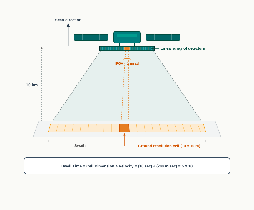
Fig. 6.9 – A pushbroom scanner recording a line.
How The Two Scanners Differ
The two scanners reach the same result by opposite means. A whiskbroom scanner uses one detector and a rotating mirror that sweeps it back and forth across the scene, building the image line by line as the mirror swings. A pushbroom scanner uses a whole row of fixed detectors, one for each ground cell, so that an entire line is captured at once with no moving part, and the image grows as the satellite flies forward. What they share is the essentials of a scanner: both are non-photographic sensors, and both assemble a digital image cell by cell from the energy reflected by the ground.
6.4 Resolving Powers Of The Satellites
A satellite’s usefulness lies not only in the detail it sees on one pass, but in its ability to return to the very same place again and again. In satellite remote sensing, the sun-synchronous polar orbit makes this possible: it lets images of the same area be collected after a fixed, pre-determined interval.
This interval is called the temporal resolution, or the revisit time of the satellite over the same area of the Earth’s surface. A satellite with a short revisit time comes back to a place often; one with a long revisit time returns only after many days.
Why Revisiting Matters
The value of coming back is change detection. Because the satellite crosses the same ground at regular gaps, two images of one place taken at different times can be laid side by side, and whatever has altered between them stands out at once. Nothing on the ground has to be measured by hand; the change reveals itself in the comparison.
Watching A Season Turn
Figure 6.10 shows this for vegetation. Two images of the Himalayas — the great mountain range along India’s northern edge — and the Northern Indian Plain below them were taken by an IRS satellite, one in May and one in November.
The two dates catch the vegetation in two different states. The red patches in the May image mark coniferous vegetation — needle-leaved trees that stay green through the year. In the November image, additional red patches appear, showing deciduous plants, which carry broad leaves that change with the season, while the lighter red is related to the crops then in the fields. Only by returning to the same area at a later date could the satellite record this seasonal shift.
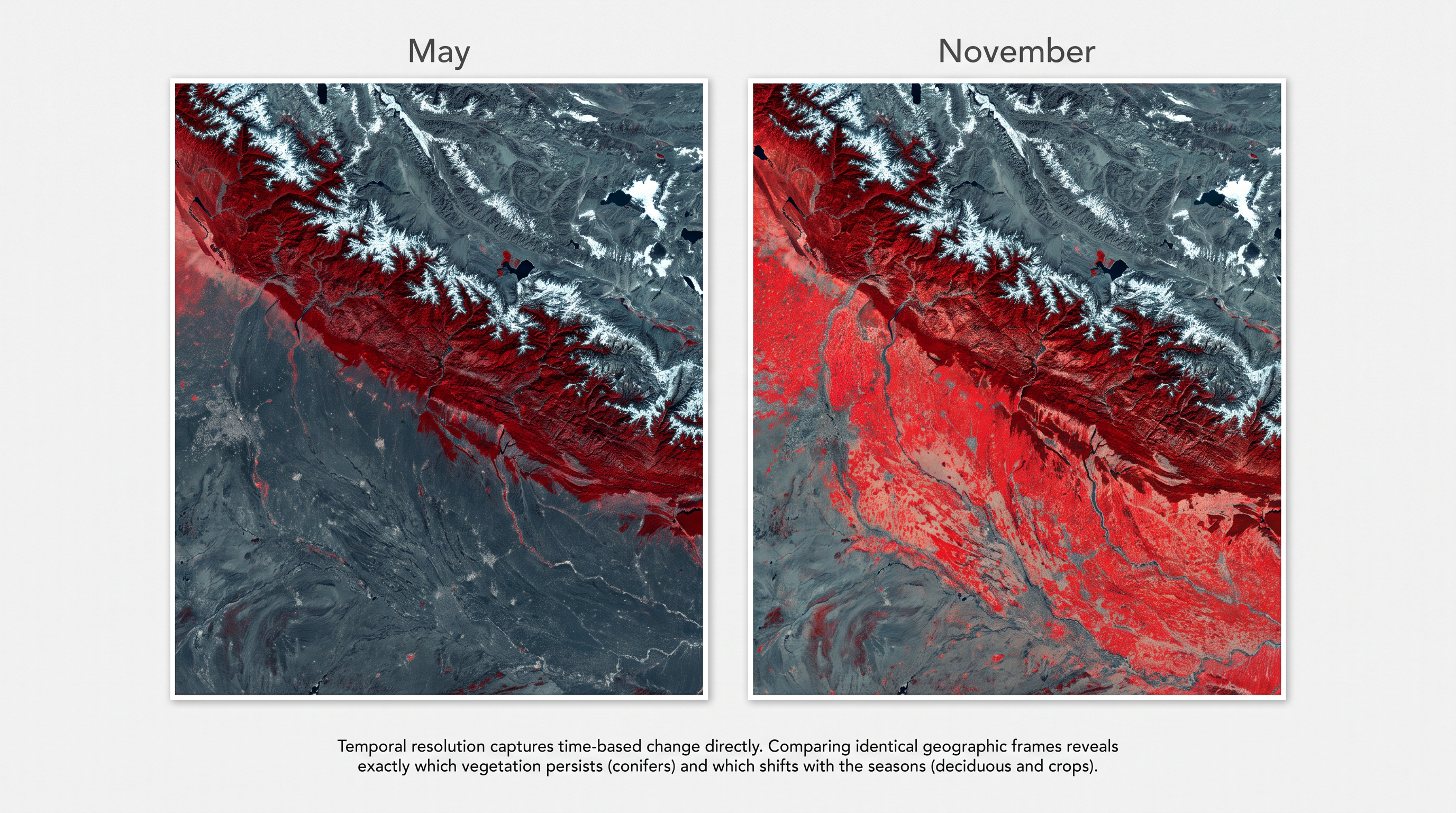
Fig. 6.10 – Himalayas in May and November.
Watching A Disaster
The same revisit ability serves a more sombre purpose in Figure 6.11. A satellite recorded the coast of Banda Aceh, in Indonesia, in June 2004, and again in December 2004 — before and after the tsunami struck that coast. The first image shows the undisturbed topography of the town; the second, acquired after the wave, reveals the damage it caused to the same ground.
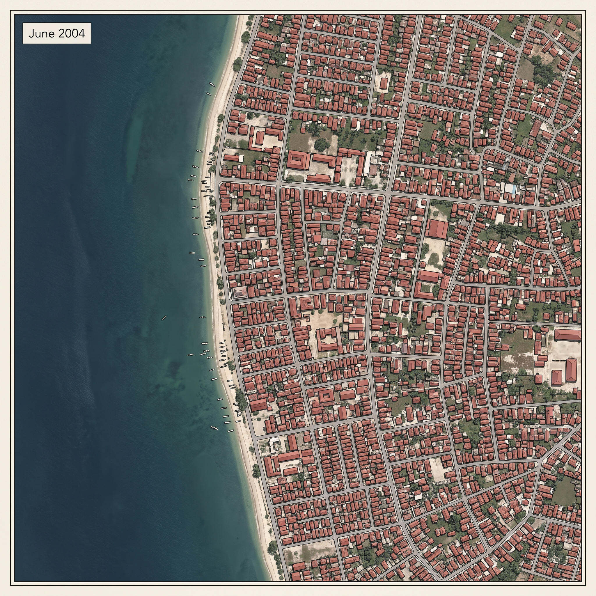
Fig. 6.11a – Pre-tsunami Banda Aceh, June 2004.
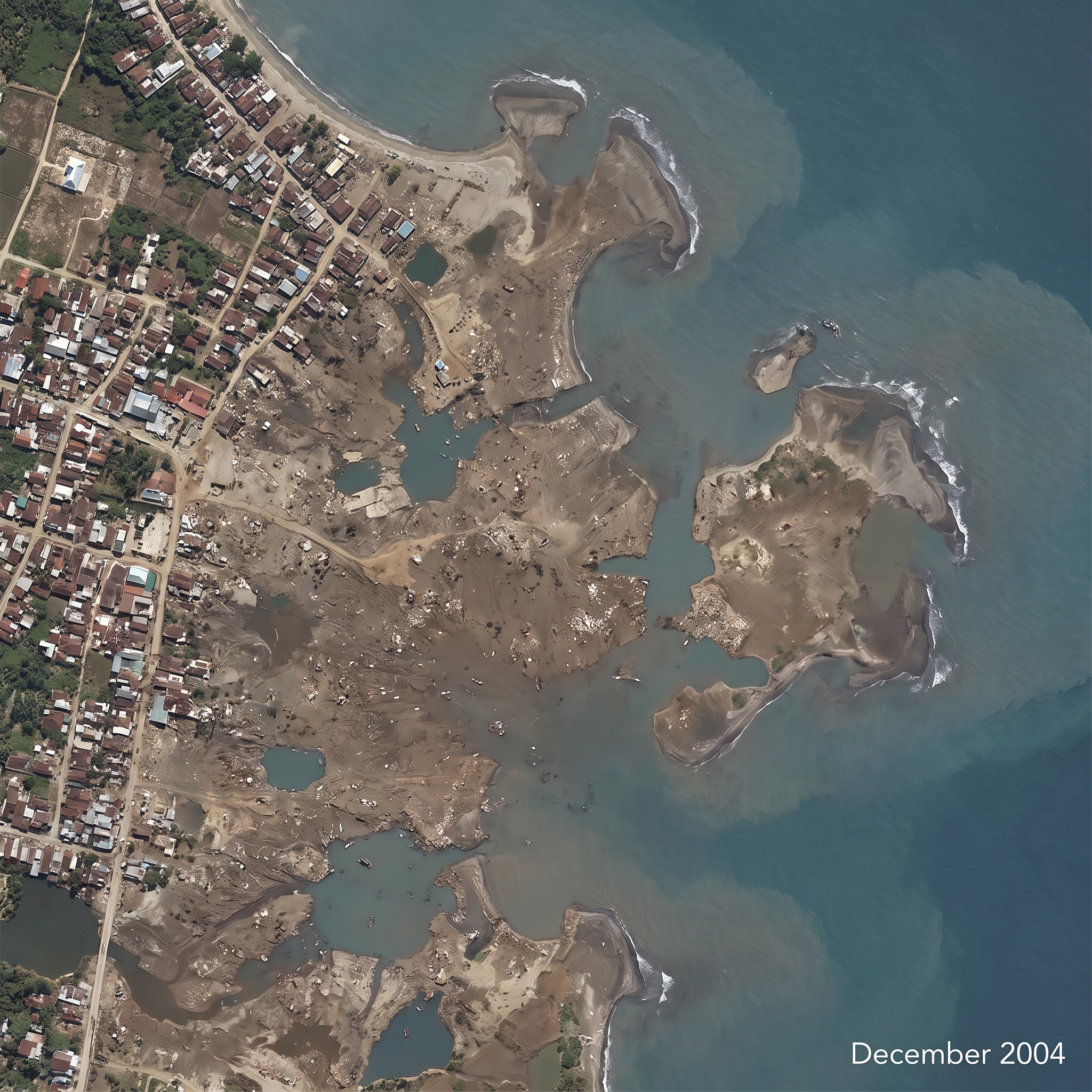
Fig. 6.11b – Post-tsunami Banda Aceh, December 2004.
6.5 Sensor Resolutions
A sensor is judged not by one quality but by several, and these together are called its resolutions. Remote sensors are characterised by their spatial, spectral and radiometric resolutions, and each of these lets useful information be pulled out for different terrain conditions. The revisit ability met in the last section — temporal resolution — is a fourth. The three taken up here describe not how often a sensor returns, but how well it sees when it does.
6.5.1 Spatial Resolution
Think of a person who wears spectacles to read. Without them, the eye cannot separate two closely spaced letters in a word and reads them as one blur; the resolving power of the eye is not enough. Positive spectacles improve that resolving power so the two letters come apart.
Spatial resolution in remote sensing works on exactly this idea. It is the capability of a sensor to distinguish two closely spaced object surfaces as two different object surfaces, rather than merging them into one. As a rule, the higher the resolution, the smaller the objects the sensor can pick out. A sensor with a spatial resolution of a few metres can separate a house from its neighbour; one with a resolution of tens of metres would see only a single grey block where a cluster of houses stands.
6.5.2 Spectral Resolution
Spectral resolution refers to the sensing and recording power of a sensor across the different bands of electromagnetic radiation. A sensor of high spectral resolution can record many narrow bands separately, instead of lumping a wide stretch of the spectrum together.
Multispectral images are obtained using a device that disperses the radiation the sensor receives and records it with detectors, each detector made sensitive to a specific spectral range. The principle behind this is the dispersion of light — the same spreading of light seen in nature as the rainbow, and produced in the laboratory with a prism.
As noted in the interaction stage earlier in this chapter, one object responds differently in different regions of the spectrum. A sensor with good spectral resolution turns that fact into information, because it records each band on its own. Figure 6.12 shows this for parts of Najafgarh, on the south-western edge of Delhi, imaged by IRS P-6 (Resourcesat-1). The same ground looks quite different from band to band: fresh water absorbs strongly and appears dark in band 4 (Infrared), while dry surfaces give a mixed strong reflectance and appear bright in band 2 (green).
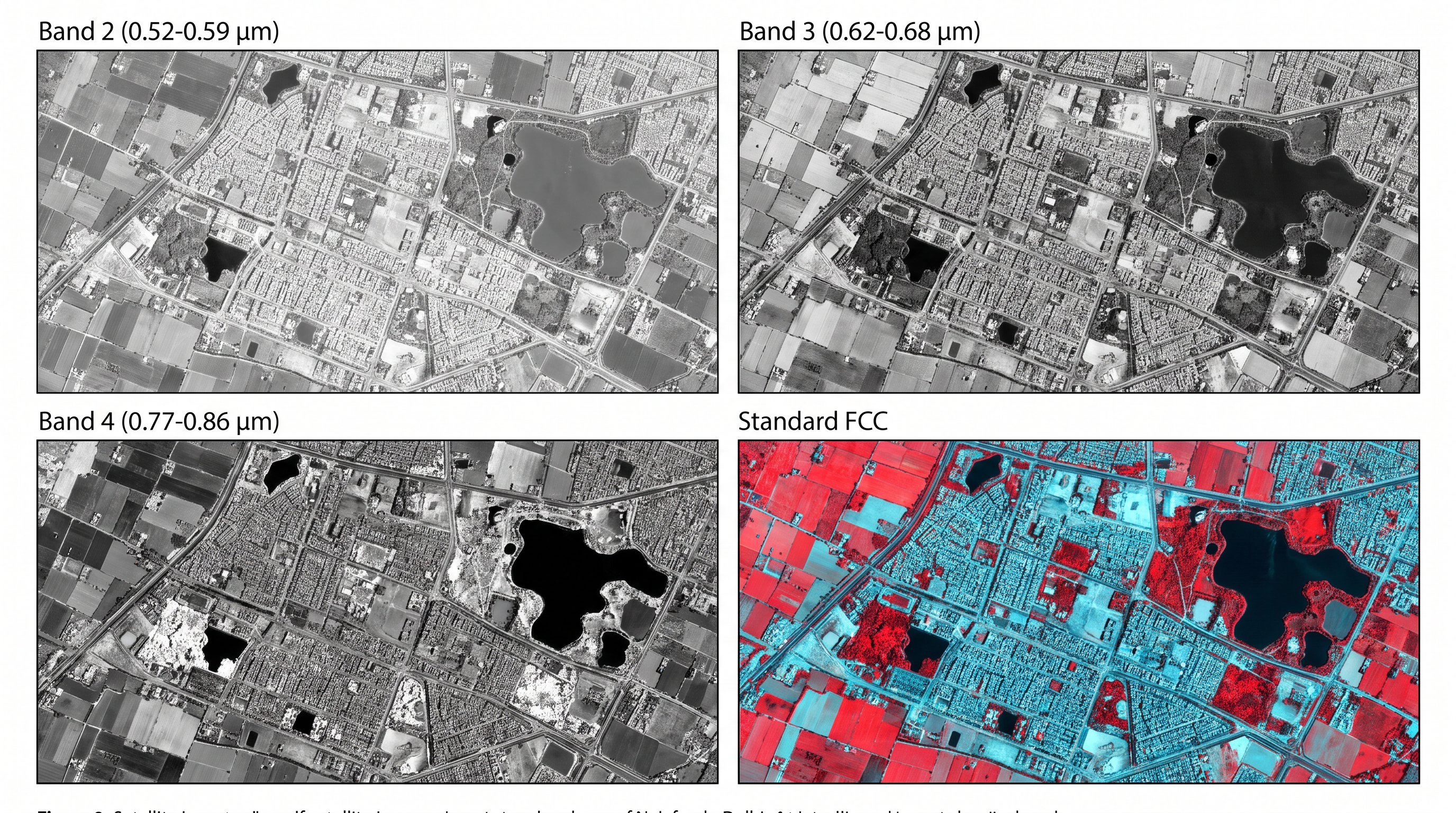
Fig. 6.12 – Najafgarh in three bands and standard FCC.
6.5.3 Radiometric Resolution
Radiometric resolution is the capability of a sensor to discriminate between two targets on the basis of how much energy each returns. The higher the radiometric resolution, the smaller the difference in radiance the sensor can detect between two targets — so two surfaces that are only slightly different in brightness can still be told apart.
The spatial, spectral and radiometric resolutions of some of the remote sensing satellites of the world are gathered in Table 6.1, so the three can be compared across sensors at a glance.
6.6 Data Products
The electromagnetic energy that a sensor gathers can be detected in two ways — photographically or electronically. The photographic process uses light-sensitive film to detect and record the variations in energy. A scanning device, on the other hand, obtains its images in digital mode.
Image Or Photograph?
Before going further it helps to separate two words that are often used as if they meant the same thing. An image is any pictorial representation of a scene, whatever region of energy was used to detect and record it. A photograph is narrower: it is an image that has specifically been recorded on photographic film. It follows that all photographs are images, but not all images are photographs — a digital scan of the same scene is an image, yet it is not a photograph.
Based on the mechanism used to detect and record them, remotely sensed data products fall into two broad types: photographic images and digital images.
6.6.1 Photographic Images
Photographs are acquired in the optical region of the electromagnetic spectrum, roughly 0.3 to 0.9 µm — the stretch that covers visible light and the near-infrared just beyond it.
Four different light-sensitive film emulsion bases are used to obtain photographs: black and white, colour, black and white infrared, and colour infrared. In aerial photography, black and white film is normally the one used.
A useful property of a photograph is that it may be enlarged to any extent without losing its information content or its contrast — blow it up and the detail holds. This is worth keeping in mind, because a digital image behaves quite differently, as the next part shows.
6.6.2 Digital Images
A digital image is not made of film grain but of discrete picture elements called pixels. Each pixel in an image has two things: an intensity value, and an address — its row-and-column position in the two-dimensional space of the image.
The intensity of a pixel is carried by a digital number (DN), which stands for the average intensity value of that pixel. The DN depends on two things: the electromagnetic energy the sensor received from that patch of ground, and the number of intensity levels used to describe the range of brightness.
Pixels And Sharpness
In a digital image, how well the detail of the objects comes through is decided by the size of the pixel. A smaller pixel generally preserves the scene’s detail better and gives a truer digital representation. But there is a limit: zoom a digital image in beyond a certain point and information is lost — the picture breaks down into the squares of the pixels themselves, and you see the grid rather than the scene. This is the opposite of a photograph, which enlarges cleanly; a digital image enlarges only so far before the pixels take over.
Using digital image processing algorithms, the digital numbers that hold each pixel’s intensity level can be displayed, as in Figure 6.13.
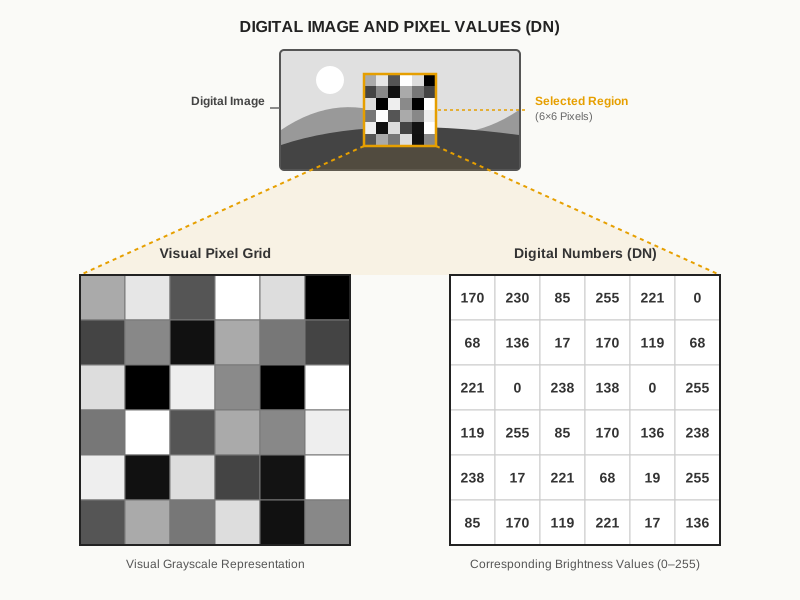
Fig. 6.13 – A digital image with pixel brightness and DN values.
6.7 Interpretation Of Satellite Imageries
The data a sensor gathers is only raw material. Its point is information extraction — working out the forms and patterns of the objects and phenomena on the Earth’s surface. Since sensors deliver both photographic and digital data products, both the qualitative and the quantitative properties of features can be drawn out, in one of two ways.
The two ways are visual interpretation and digital image processing. Visual interpretation is a manual exercise: a person reads the image of an object in order to identify it. Digital image processing is not manual at all; it needs a combination of hardware and software to extract the desired information. Working through digital image processing is not possible here, given the demands of time, equipment and accessories, so this chapter keeps to visual interpretation alone.
6.7.1 Elements Of Visual Interpretation
Whether we notice it or not, we already read the world this way. To recognise an object in daily life we use its form, its size, its location, and its relationship with the objects around it. These characteristics, used deliberately to read an image, are the elements of visual interpretation.
They fall into two groups. The image characteristics are the ones read from the image itself — the tone or colour an object shows, its shape, its size, its pattern, its texture and the shadow it casts. The terrain characteristics are read from the object’s setting — its location, and its association with the surrounding objects. The seven elements below run through both groups.
6.7.1.1 Tone Or Colour
All objects receive energy in all regions of the spectrum, and the interaction of that energy with an object leads to absorption, transmittance and reflection. It is the reflected part that the sensor receives and records — as tone, the shades of grey in a black-and-white image, or as colour, the hues in a colour image.
The tone or colour an object shows depends on three things: the orientation of the incoming radiation, the surface properties of the object, and its composition. As a broad rule, smooth and dry surfaces reflect more energy than rough and moist ones, so they appear lighter. On top of this, the same object responds differently in different regions of the spectrum.
Healthy vegetation is the classic example. It reflects strongly in the infrared region because of its multiple-layered leaf structure, so in a standard false colour composite it appears in a light tone, a bright red; scrubs appear in a greyish red. Water behaves the opposite way. A fresh water body absorbs much of the radiation it receives and appears in a dark tone or black, while a turbid water body appears in a light tone or light bluish colour in an FCC, because its suspended sand particles and water molecules together give a mixed response. Figures 6.14 (a) and (b) show a turbid and a fresh-water river for comparison.
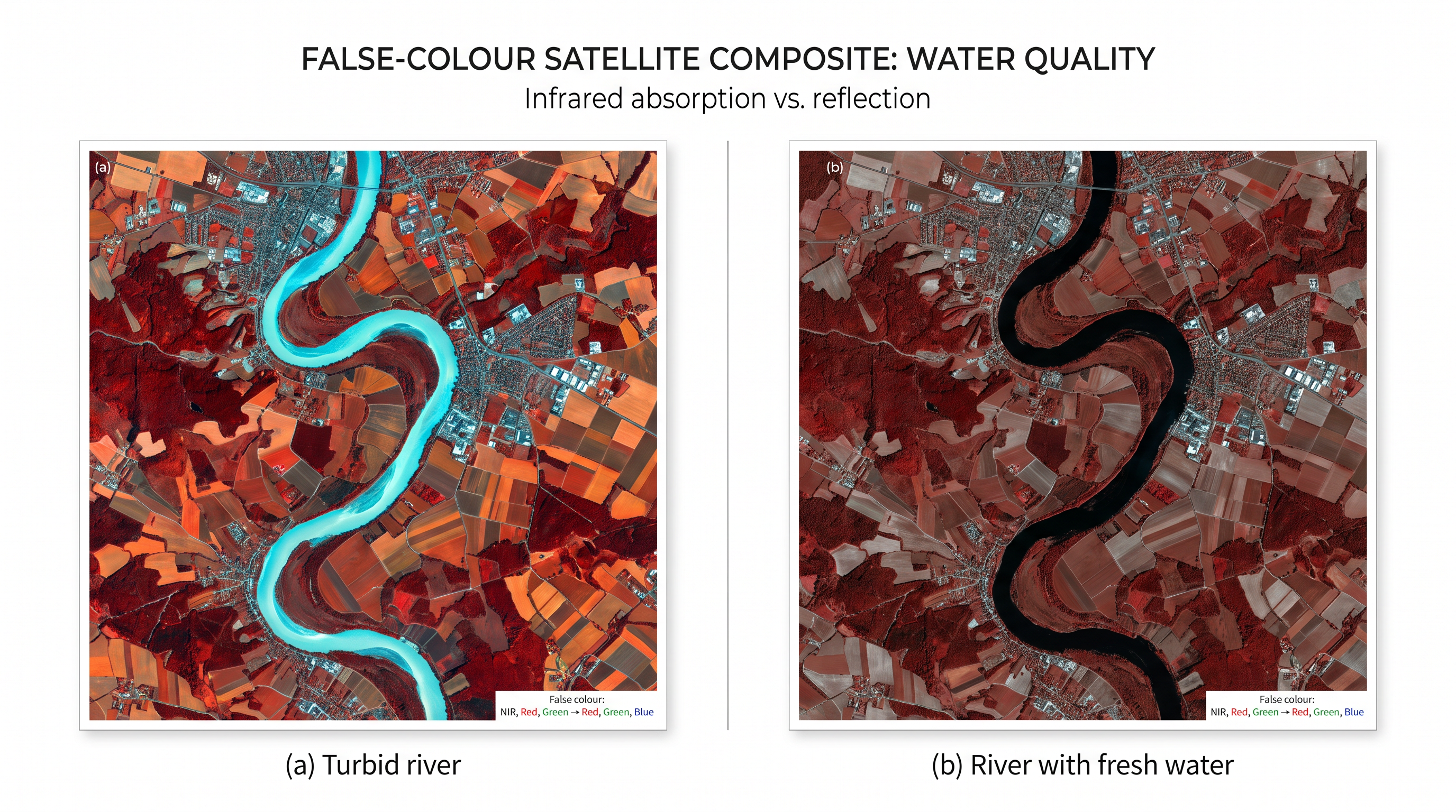
Fig. 6.14 – Tone difference: (a) turbid and (b) fresh water.
The colours that different features of the Earth’s surface take in a standard false colour composite are gathered in Table 6.2.
6.7.1.2 Texture
Texture refers to the minor variations within the tones of grey or the hues of colour. These small variations are caused by an aggregation of features too small to be picked out one by one — the mix of high-density and low-density housing, slums and squatter settlements, garbage and other solid waste, and different crops and plants. Together, such small units give a surface a texture that runs from smooth to coarse.
The differences are readable. Dense residential areas in a large city form a fine texture, because the houses are packed close in a small area, while low-density areas produce a coarse texture. In high-resolution images, sugarcane or millet plants give a coarse texture next to the fine texture of rice or wheat. Scrubbed lands, likewise, read as coarse against the fine texture of lush green evergreen forest. Figures 6.15 (a) and (b) set a coarse and a fine texture side by side.
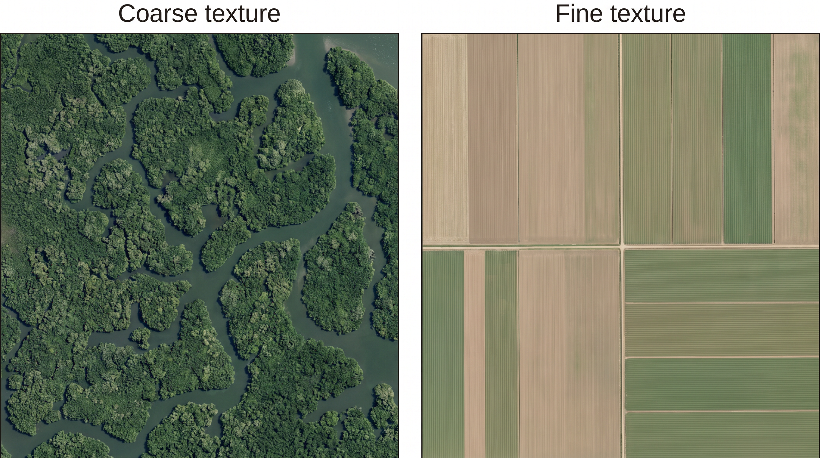
Fig. 6.15 – Texture difference: (a) mangroves and (b) cropped land.
6.7.1.3 Size
The size of an object, as judged from the resolution or scale of an image, is another important clue. It helps tell apart features that would otherwise look similar — industrial buildings and industrial complexes from residential dwellings, a stadium in the heart of a city from brick kilns at its fringe, and the size and hierarchy of settlements. Figures 6.16 (a) and (b), of parts of Kolkata in eastern India and Varanasi on the Ganga in the north, show how the size difference between institutional buildings and residential areas can be read directly from the image.
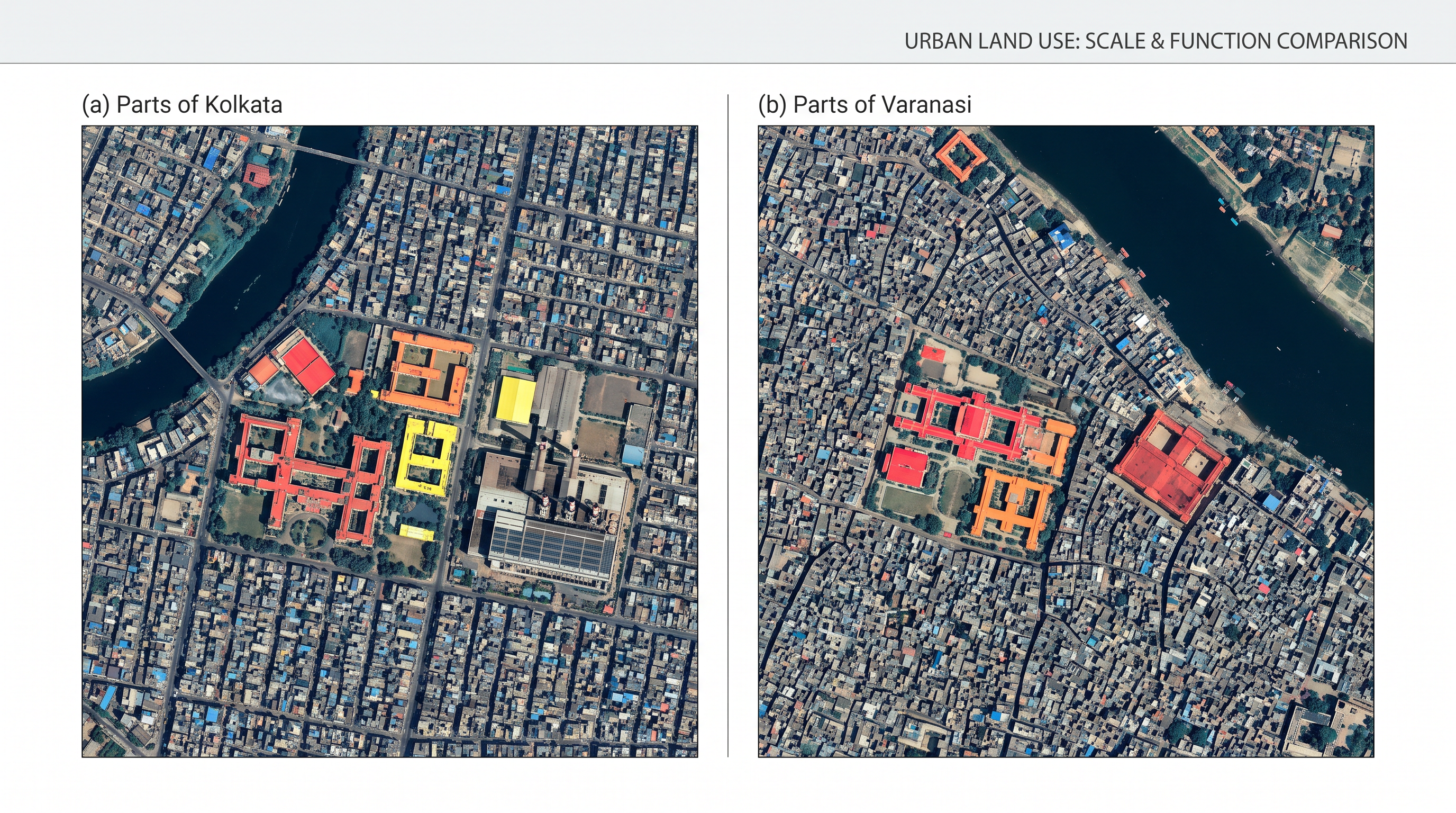
Fig. 6.16 – Size difference in (a) Kolkata and (b) Varanasi.
6.7.1.4 Shape
The shape of an object — its general form, configuration or outline — often gives it away at once. Some shapes are so distinctive that they identify the object by themselves. The outline of the Sansad Bhawan, the Parliament building in New Delhi, is unlike almost any other built-up feature. A railway line can be told from a road by its long, continuous linearity and the gradual change in its course, as Figure 6.17 shows. Shape also helps mark out religious places such as mosques and temples as distinct features.
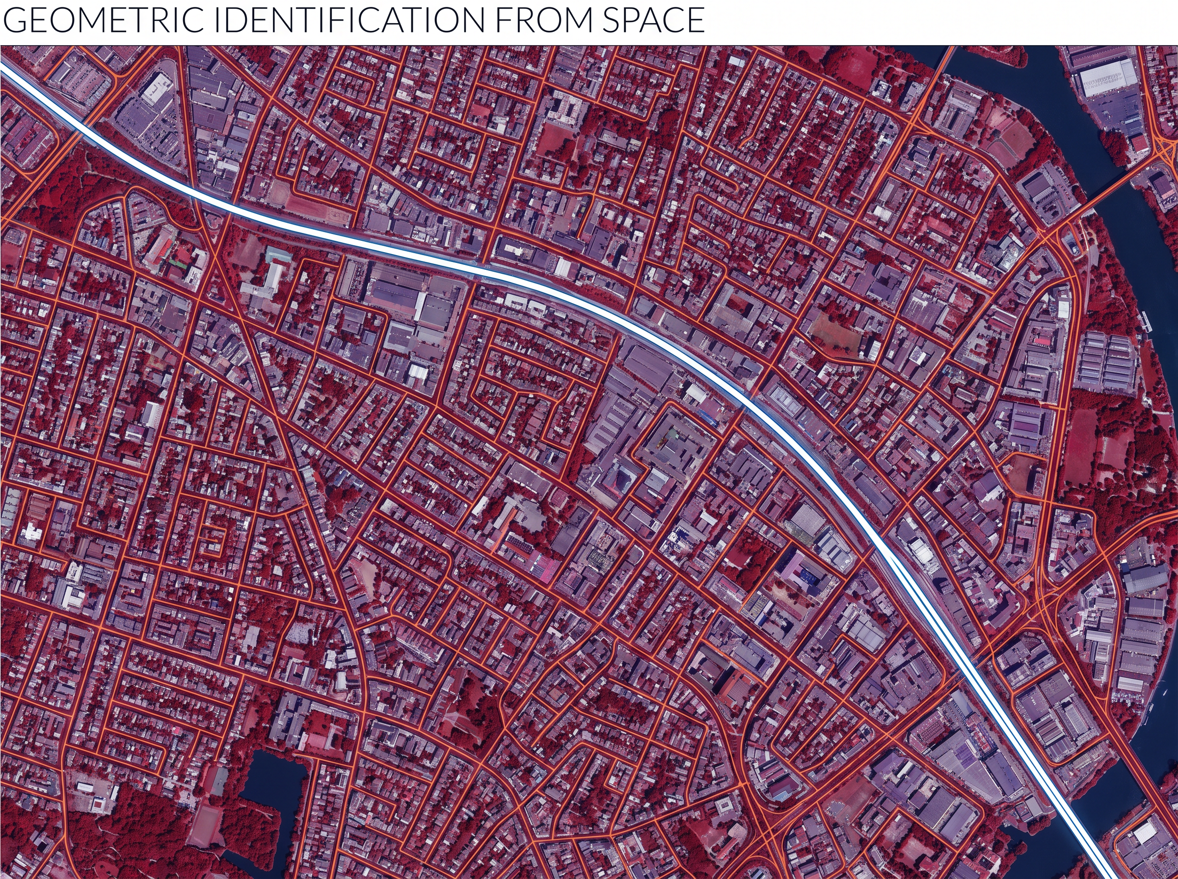
Fig. 6.17 – Railway track and roads in an urban area.
6.7.1.5 Shadow
A shadow is a function of the Sun’s illumination angle and the height of the object casting it. Some objects are so shaped that they cannot be identified without reading the length of their shadow. The Qutub Minar, a tall tower in Delhi, the minarets of mosques, overhead water tanks, and electric or telephone lines are recognised in this way.
Shadow cuts both ways. In city centres it can work against identification, because a tall building throws a dark tone that swamps the true tone or colour of whatever lies beneath it. As an element, shadow is of less use in satellite images, but it serves a useful purpose in large-scale aerial photography, where objects are large enough for their shadows to tell.
6.7.1.6 Pattern
Many natural and man-made features are laid out in a pattern — a repetitive arrangement of forms and relationships — and the pattern itself becomes the clue. Planned residential areas, with dwelling units of the same size and layout, are easily identified once their pattern is followed, as in Figure 6.18. Orchards and plantations show the same type of plant at uniform inter-plant distances. Different types of drainage, or of settlement, can likewise be distinguished if their pattern is studied and recognised.
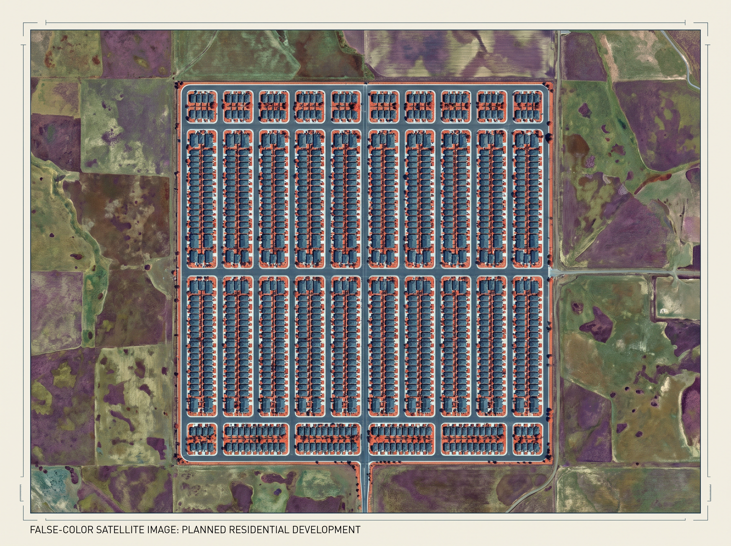
Fig. 6.18 – The regular pattern of a planned residential area.
6.7.1.7 Association
Association is the relationship between objects and their surroundings, together with their geographical location. Certain features are found reliably near certain others. An educational institution is usually near a residential area and has a playground within its premises. A stadium, race course or golf course goes with a large city; industrial sites gather along a highway at the edge of a growing city; and slums often line the drains and railway tracks. Reading these associations, an interpreter identifies a feature not on its own but by the company it keeps.
For readers who wish to go further, the chapter points to three official Indian sources — the Indian Space Research Organisation (isro.gov.in), the National Remote Sensing Centre (nrsc.gov.in) and the Indian Institute of Remote Sensing (iirs.gov.in).
6.8 Summary
- Remote sensing is the set of processes that acquire information about an object from a distance, using a sensor that is not in physical contact with it. It always needs three things: an object surface, a sensor, and information-carrying energy waves between them.
- The process runs as a chain of eight stages, from a source of energy to a finished map or table.
- The Sun is the main source of energy; energy can also be generated artificially, as in radar.
- Energy travels as electromagnetic radiation at the speed of light. Its variations make up the electromagnetic spectrum, of which the visible, infrared and microwave regions are used in remote sensing.
- On reaching the surface, energy is absorbed, transmitted, reflected or emitted, and each surface reflects differently across the bands — its spectral signature, which lets a sensor tell surfaces apart.
- As reflected energy returns through the atmosphere, gases, water molecules and dust absorb or scatter some of it, so that part of the information is left unrecorded.
- Remote sensing satellites fly low in a sun-synchronous orbit (700 to 900 km) for fine detail, such as the IRS series; weather and telecommunication satellites sit far out in a geostationary orbit (about 36,000 km) for a wide, constant view, such as INSAT.
- The received energy is converted to digital or photographic data, transmitted to an Earth Receiving Station, corrected, interpreted, and turned into thematic maps and tables.
- Sensors are photographic (cameras) or non-photographic (scanners). Multispectral scanners come as whiskbroom scanners, which sweep one detector with a rotating mirror, and pushbroom scanners, which use a fixed row of detectors.
- A sensor’s quality is described by its spatial, spectral, radiometric and temporal (revisit) resolutions.
- Data products are photographic images or digital images; a digital image is a grid of pixels, each holding a digital number for its brightness.
- Information is extracted here by visual interpretation, reading seven elements — tone or colour, texture, size, shape, shadow, pattern and association.
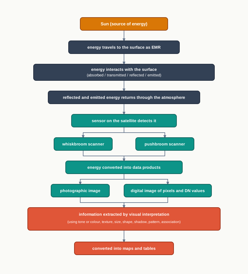
Fig. 6.19 – The remote sensing data acquisition chain.
What This Chapter Cannot Tell You
- The chapter teaches only visual interpretation; the digital image processing that does much of the real work is set aside, so the reader sees the manual half of interpretation, not the automated one.
- The resolution figures and satellite specifications are design values. They say what a sensor is built to do, not what any single image will actually reveal on a given day.
- A false colour composite’s colour signatures are typical, not certain, and a pair of before-and-after images shows that a change happened, never why it happened — the ground reason lies outside the image.
6.9 NCERT Questions
Remote sensing of objects can be done through various means such as A. remote sensors, B. human eyes and C. photographic system. Which of the following represents the true order of their evolution?
- ABC
- BCA
- CAB
- None of the above
Which of the following regions of the electromagnetic spectrum is not used in satellite remote sensing?
- Microwave region
- Infrared region
- X-rays
- Visible region
Which of the following is not used in the visual interpretation technique?
- Spatial arrangements of objects
- Frequency of tonal change on the image
- Location of objects with respect to other objects
- Digital image processing
Why is remote sensing a better technique than other traditional methods?
Differentiate between IRS and INSAT series of satellites.
Describe in brief the functioning of a pushbroom scanner.
Describe the operation of a whiskbroom scanner with the help of a diagram. Explain how it is different from a pushbroom scanner.
Identify and list the changes that can be observed in the vegetation of the Himalayas (Fig. 6.10).
Identify the various features marked on the IRS IC LISS III imagery shown in the chapter. Draw clues from the elements of image interpretation discussed and the colours in which various objects appear on a standard false colour composite.
6.10 Check Your Concepts
List, in order, the eight stages by which remote sensing data is acquired, from the source of energy to the final map or table.
Using Table 6.2, state the colour that clear water and a high-density built-up area each take on a standard false colour composite, and suggest why the two differ.
In Fig. 6.13, what does each number in the array stand for, and what would a value of 255 and a value of 0 tell you about their pixels?
From the spectral signatures in Fig. 6.5, which surface reflects most strongly in the near-infrared? Use this to explain why a fresh water body appears dark in an infrared band.
Distinguish spatial resolution from radiometric resolution. Can a sensor have fine spatial resolution but coarse radiometric resolution? Explain.
From Table 6.1, identify the sensor with the finest spatial resolution and the one with the widest radiometric range, and explain what each of these means for the image.
The chapter gives the SPOT HRVR-1 sensor a swath of 60 km and a spatial resolution of 20 metres. Work out the number of detectors it needs, showing every step of the calculation.