Chapter 3: Current Electricity
For most of human history, the only electricity people could produce was a brief, dramatic spark. Rub a glass rod with silk, and it would crackle, attract bits of paper, or give a sudden shock — but the effect vanished in an instant. Electricity seemed to be something that arrived and left in a flash, never something that could be made to flow steadily, the way water flows in a river.
That changed around the year 1800, when the Italian scientist Alessandro Volta built a device that would quietly reshape the modern world. Volta stacked alternating discs of zinc and copper, separating each pair with cloth soaked in salty water. This simple “pile,” as he called it, did something no rubbed rod or spark could do: it pushed charge around a connected wire continuously, producing the first steady electric current in history.
Volta had been arguing with a fellow scientist, Luigi Galvani, about why a dead frog’s leg twitched when touched by two different metals. Galvani thought the electricity came from the animal. Volta suspected the metals themselves were the source — and his pile proved him right. For the first time, humans had a reliable “pump” for charge. Nearly every electrical device you use today, from a torch to a smartphone, is a descendant of that pile.
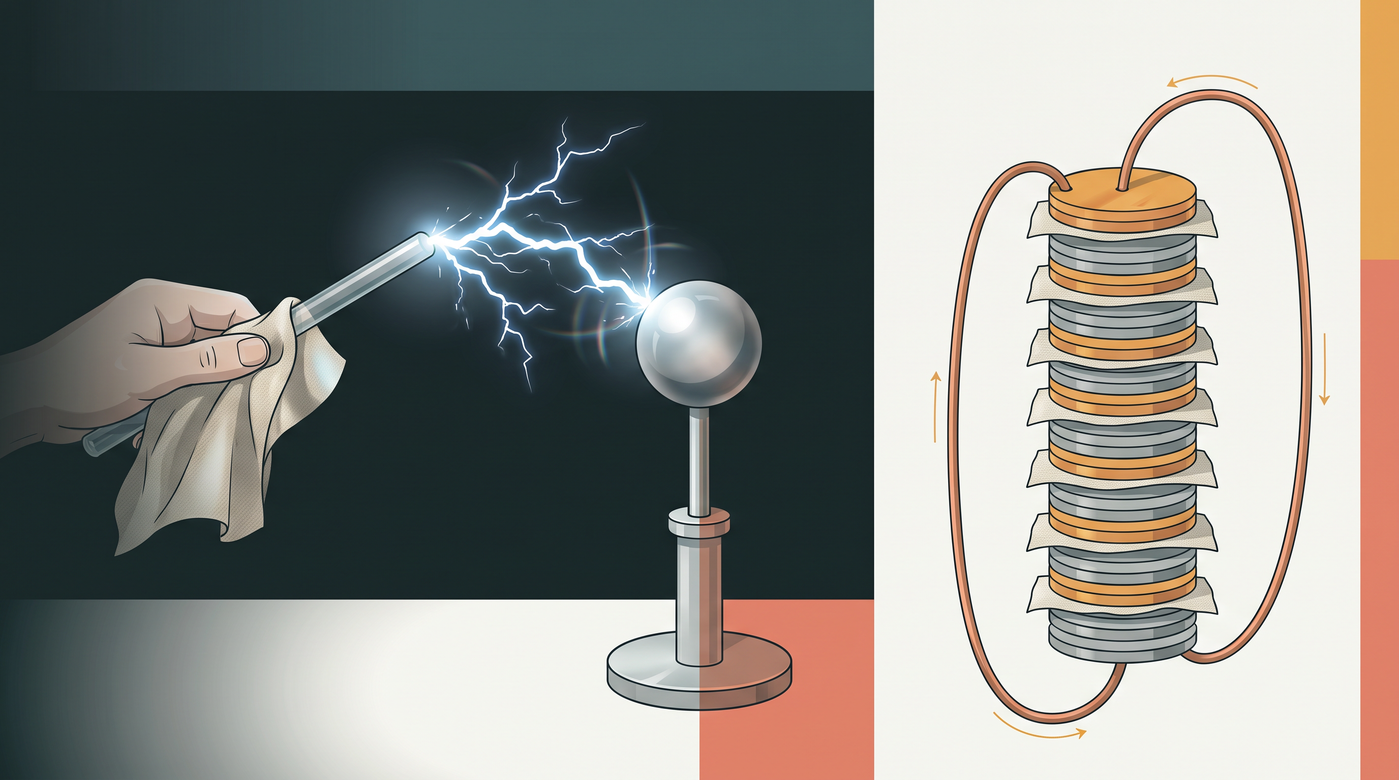
Fig. 3.0 – Volta’s pile and a static spark.
By the end of this chapter, you will be able to answer each of these questions using the basic laws that govern steady electric currents.
3.1 Introduction
In Chapter 1, we studied electrostatics — the physics of charges that stay put. There, every charge, whether it was free to move or bound inside a material, was treated as being at rest. We looked at the forces between such charges and the fields they set up, but nothing actually flowed.
In this chapter we take the next natural step and let charges move. When charges are in motion, their flow is called an electric current. This single idea — moving charge — is the foundation of almost every electrical device around you.
Currents are not something we create only in laboratories; they occur in nature too. Lightning is a striking example. During a storm, enormous amounts of charge build up in the clouds, and when the buildup becomes large enough, charge suddenly rushes from the clouds to the earth through the air, sometimes with destructive results.
Notice, however, that the flow in lightning is sudden and short-lived — it is not steady. In everyday life we usually deal with a very different kind of flow: one that continues smoothly and evenly, much like water moving steadily down a river rather than a flash flood. A torch and a cell-driven clock are simple examples of devices in which charge flows in this steady, controlled manner.
It is this steady flow that we care about most. In the present chapter, we shall study the basic laws that govern steady electric currents — how to measure them, what controls their size, how they lose energy as heat, and how the sources that drive them behave.
3.2 Electric Current
In the previous section we said that current is the flow of charge. To turn that idea into something we can actually measure, we need to be precise about how much charge flows and how fast it flows. That is what this section does.
Imagine holding a small flat area inside a region where charges are moving, and orient this area so that it faces the flow squarely — that is, the area is held normal (perpendicular) to the direction in which the charges move, as shown in Fig. 3.1. Charges will cross this area as they travel.
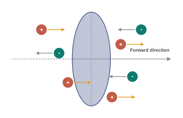
Fig. 3.1 – Flow of charge across an area.
Now, both positive and negative charges may cross this area, and they may cross in either direction — some go forward, some may drift backward. To keep track, we count the net movement, meaning forward crossings minus backward crossings.
In a given time interval \(t\), let \(q_+\) be the net amount of positive charge that crosses the area in the forward direction (forward minus backward). Similarly, let \(q_-\) be the net amount of negative charge that crosses in the forward direction. Here \(q_+\) and \(q_-\) are measured in coulombs (C), the SI unit of charge.
The total net charge that crosses the area in the forward direction during time \(t\) is then the sum of these contributions: \[q = q_+ - q_-\]
For a steady current — one that does not change with time — this net charge \(q\) is proportional to the time \(t\): let it flow for twice as long and twice as much charge crosses. Because of this proportionality, the ratio of charge to time is a fixed number, and we define this ratio to be the current: \[I = \frac{q}{t} \tag{3.1}\]
Here \(I\) is the electric current (SI unit: ampere, A), \(q\) is the net charge crossing the area (coulomb, C), and \(t\) is the time interval (second, s).
Equation (3.1) works well when the current is steady. But currents are not always steady; they can rise and fall from moment to moment. For such cases we need a more general definition that gives the current at a particular instant.
To do this, we look at a very short time interval. Let \(\Delta Q\) be the net charge flowing across a cross-section of a conductor during the small time interval \(\Delta t\), that is, between times \(t\) and \((t + \Delta t)\). The average current over that interval is \(\Delta Q/\Delta t\). To get the current at the instant \(t\), we shrink the interval \(\Delta t\) towards zero, taking the limit: \[I(t) \equiv \lim_{\Delta t \to 0} \frac{\Delta Q}{\Delta t} \tag{3.2}\]
In words, the instantaneous current is the value that the ratio \(\Delta Q/\Delta t\) approaches as the time interval \(\Delta t\) becomes vanishingly small. This is the same limiting idea used to define instantaneous speed in mechanics, applied here to charge instead of distance.
In SI units, the unit of current is the ampere (symbol A). The ampere is actually defined through the magnetic effects that currents produce — an effect we will study in the following chapter — rather than through charge and time directly. For now, you can simply treat the ampere as the practical unit in which currents are measured.
It helps to get a feel for the range of currents found in the world around us. An ampere is typically the order of magnitude of the currents that flow in ordinary domestic appliances. At the high extreme, an average lightning strike carries a current of the order of tens of thousands of amperes. At the low extreme, the tiny currents that travel along the nerves in our body are only of the order of microamperes (\(1\ \mu\text{A} = 10^{-6}\ \text{A}\)). So the currents we deal with span an enormous range — many orders of magnitude — from feeble nerve signals to violent atmospheric discharges.
3.3 Electric Currents in Conductors
We now ask a practical question: which materials actually allow a current to flow, and why? The answer lies in whether a material contains charges that are free to move.
Recall from Chapter 1 that an electric charge placed in an electric field feels a force. (An electric field is simply the region around charges in which another charge would experience a force; we represent its strength and direction by the vector \(\vec{E}\).) If the charge is free to move, this force sets it moving — and moving charge is exactly what we call a current. So the key requirement for a current is the presence of charges that can move freely.
Do such free charges exist in nature? Yes. In the upper layers of the atmosphere, called the ionosphere, charged particles do roam freely. But in ordinary atoms and molecules the situation is different: the negatively charged electrons and the positively charged nuclei are bound to each other by electrical attraction, so they are not free to wander off.
Bulk matter is built from a huge number of such molecules. A single gram of water, for instance, contains roughly \(10^{22}\) molecules. In a solid, these molecules are packed so closely together that the outer electrons are no longer tied to any one particular nucleus.
What happens next depends on the material. In some materials the electrons remain bound — they will not accelerate even when an electric field is applied. Such materials are insulators. In other materials, most notably metals, a fraction of the electrons are practically free to move throughout the whole piece of material. These materials are called conductors, and it is they that develop electric currents when an electric field is applied.
If we look specifically at solid conductors, the atoms are locked tightly in place, so the current cannot be carried by them. Instead it is carried by the negatively charged electrons that are free to move. There are other kinds of conductors too — for example, electrolytic solutions, in which both positive and negative charges can move. To keep our discussion simple, we will focus only on solid conductors, where the current is carried by free electrons moving against a fixed background of positive ions.
What happens with no electric field
Consider first the case when no electric field is present in the conductor. The free electrons are not sitting still — because of their temperature, they are in constant, restless motion. This temperature-driven jiggling is called thermal motion. As they move, the electrons repeatedly collide with the fixed positive ions.
An important point about these collisions: an electron that strikes an ion bounces off with the same speed it had before, but in a completely random new direction. There is no direction that the electrons prefer over any other.
Because the directions are random, at any given instant the number of electrons heading one way is matched, on average, by an equal number heading the opposite way. Their velocities cancel out. So, on the whole, there is no net flow of charge in any particular direction — and therefore no electric current.
What happens when an electric field is applied
Now let us see what changes when an electric field is switched on. To picture it clearly, imagine the conductor shaped as a cylinder of radius \(R\) (Fig. 3.2). Take two thin circular discs made of an insulating (dielectric) material of the same radius. Spread a positive charge \(+Q\) over one disc and an equal negative charge \(-Q\) over the other, then attach the two discs to the two flat ends of the cylinder.
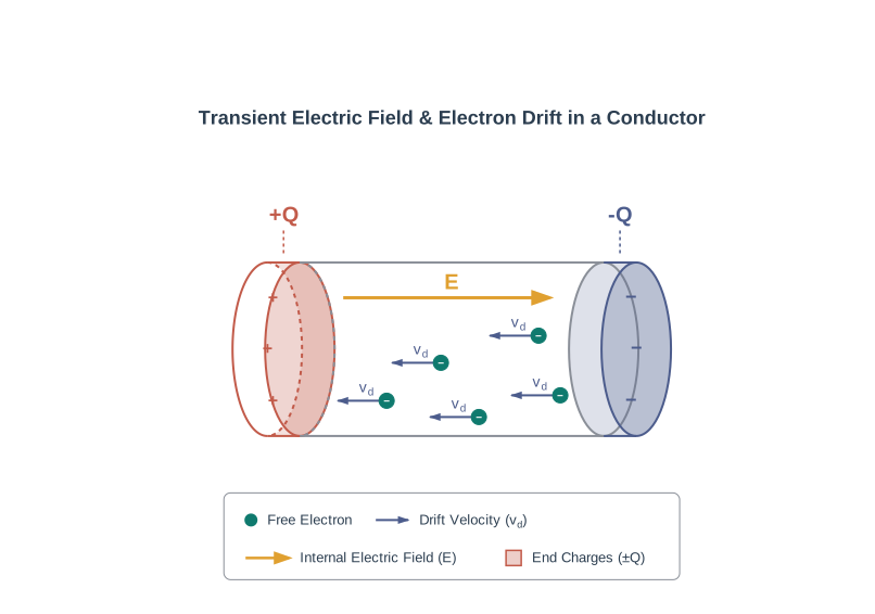
Fig. 3.2 – Electric field and electron drift in a conductor.
With these charges in place, an electric field is created inside the cylinder, directed from the positive charge towards the negative charge. The free electrons, being negative, feel a force opposite to the field and are accelerated towards the \(+Q\) end. As they move, they constitute an electric current, and they steadily neutralise the charges on the discs.
But here is the catch: as the electrons cancel out \(+Q\) and \(-Q\), the field that was driving them weakens and finally disappears. So in this arrangement there is a current only for a very short while, and then it stops. The charges get used up.
Maintaining a steady current
To keep the current flowing, we would need some mechanism that continually supplies fresh charge to the ends of the cylinder, replacing whatever the electrons neutralise. If we could do that, a steady electric field would be maintained inside the conductor, and instead of a brief burst we would get a continuous, lasting current.
Devices that maintain such a steady electric field are exactly the cells and batteries that we will study later in this chapter. This is precisely why a rubbed comb loses its charge in an instant — its charge is neutralised and never replenished — while a battery can drive a current for hours: it keeps pumping charge to sustain the field.
In the next sections, we turn to the steady current that results from a steady electric field maintained in a conductor, and the laws that govern it.
3.4 Ohm’s Law
We have seen that a steady electric field drives a steady current in a conductor. The next natural question is: how much current flows for a given “push”? The relationship between the push (the potential difference) and the resulting current was discovered experimentally by G.S. Ohm in 1828 — remarkably, long before anyone understood the underlying mechanism of how currents actually flow.
Imagine a conductor carrying a current \(I\), and let \(V\) be the potential difference between its two ends. The potential difference (measured in volts, V) is the difference in electric potential across the conductor — you can think of it as the electrical “pressure” that pushes charge through. Ohm found that the current is directly proportional to this potential difference: \[V \propto I\] or, writing the proportionality as an equation, \[V = R\,I \tag{3.3}\]
The constant of proportionality \(R\) is called the resistance of the conductor. Its SI unit is the ohm, denoted by the symbol \(\Omega\). Here \(V\) is in volts (V), \(I\) is in amperes (A), and \(R\) is in ohms (\(\Omega\)).
What does the resistance depend on?
Resistance is not just a property of the material; it also depends on the shape and size of the conductor. A long thin wire resists current more than a short thick one of the same metal. We can work out exactly how \(R\) depends on the dimensions using a simple argument.
Consider a conductor obeying Eq. (3.3), shaped as a slab of length \(l\) and cross-sectional area \(A\), as shown in Fig. 3.3(a).
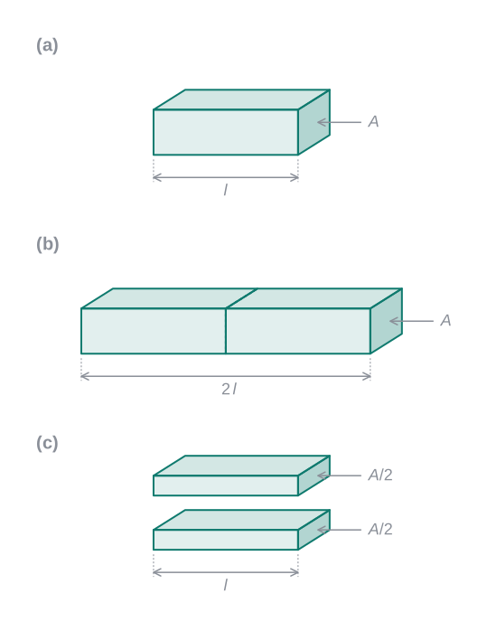
Fig. 3.3 – Dependence of resistance on dimensions.
Effect of length. Now imagine placing two identical slabs side by side, end to end [Fig. 3.3(b)], so the combined length is \(2l\). The same current \(I\) that flows through one slab flows through the whole combination. If \(V\) is the potential difference across the first slab, then the second slab — being identical and carrying the same current — also has \(V\) across it. So the potential difference across the whole combination is the sum, \(2V\).
The current through the combination is still \(I\), so by Eq. (3.3) its resistance \(R_C\) is \[R_C = \frac{2V}{I} = 2R \tag{3.4}\] since \(V/I = R\) is the resistance of a single slab. Doubling the length has doubled the resistance. In general, then, resistance is proportional to length: \[R \propto l \tag{3.5}\]
This makes physical sense: a longer conductor gives the electrons a longer path over which to suffer collisions, so it is harder for current to get through.
Effect of area. Next, take the original slab and imagine cutting it lengthwise into two, so it becomes two identical slabs each of length \(l\) but each with cross-sectional area \(A/2\) [Fig. 3.3(c)].
For a given voltage \(V\) across the slab, let \(I\) be the total current through it. By symmetry, this current splits equally, so each half-slab carries \(I/2\). The potential difference across each half-slab is still \(V\) (the same as across the full slab, since they run alongside each other). Therefore the resistance of each half-slab, \(R_1\), is \[R_1 = \frac{V}{(I/2)} = 2\frac{V}{I} = 2R \tag{3.6}\]
So halving the cross-sectional area doubles the resistance. In general, then, resistance is inversely proportional to the cross-sectional area: \[R \propto \frac{1}{A} \tag{3.7}\]
This too makes sense: a wider conductor offers more room — more parallel paths — for the electrons to flow through, so it resists less.
Combining the two results. Putting Eqs. (3.5) and (3.7) together, \[R \propto \frac{l}{A} \tag{3.8}\] and hence, for a given conductor, \[R = \rho\,\frac{l}{A} \tag{3.9}\]
The constant of proportionality \(\rho\) depends only on the material of the conductor, not on its dimensions. It is called the resistivity of the material, with SI unit ohm-metre (\(\Omega\,\text{m}\)).
Using Eq. (3.9), Ohm’s law can be rewritten in terms of the dimensions: \[V = I \times R = \frac{I\rho l}{A} \tag{3.10}\]
Current density and conductivity
It is often more useful to describe the flow not by the total current, but by how crowded that current is within the conductor. The current per unit area (with the area taken normal to the flow), \(I/A\), is called the current density and is denoted by \(j\). Its SI unit is ampere per square metre (\(\text{A/m}^2\)).
Suppose the conductor has a uniform electric field of magnitude \(E\) inside it, and its length is \(l\). Then the potential difference across its ends is \(V = El\). Substituting \(V = El\) and \(I/A = j\) into Eq. (3.10): \[E\,l = j\,\rho\,l\] and cancelling the common length \(l\) from both sides: \[E = j\,\rho \tag{3.11}\]
This relation was written for the magnitudes \(E\) and \(j\), but it can be put into vector form. The current density points along the direction of the field \(\vec{E}\), so \(\vec{j}\) is also a vector, \(\vec{j} \left(= j\,\vec{E}/E\right)\). Thus the last equation becomes \[\vec{E} = \vec{j}\,\rho \tag{3.12}\] or, rearranging, \[\vec{j} = \sigma \vec{E} \tag{3.13}\]
where \(\sigma \equiv 1/\rho\) is called the conductivity of the material, with SI unit siemens per metre (\(\text{S/m}\)). Conductivity simply measures how easily a material conducts, whereas resistivity measures how strongly it opposes; they are reciprocals of each other.
Equation (3.13), \(\vec{j} = \sigma \vec{E}\), is a very useful form of Ohm’s law. It says the current density at a point is proportional to the electric field at that point — a statement that holds locally, at every point inside the conductor, rather than just across the ends. Ohm’s law is often stated in this equivalent form, in addition to the familiar \(V = RI\) of Eq. (3.3).
In the next section, we will try to understand why Ohm’s law holds — that is, where this proportionality comes from — by looking closely at how the electrons drift through the conductor.
3.5 Drift of Electrons and the Origin of Resistivity
In the last section we accepted Ohm’s law as an experimental fact. Now we ask the deeper question: why is current proportional to voltage? To answer this, we build a simple picture of what the free electrons are actually doing inside a metal, and we will find that Ohm’s law drops out naturally.
As noted earlier, an electron in a metal keeps colliding with the heavy fixed ions. After each collision it emerges with the same speed but in a random direction. If we look at all the electrons together, their velocities point every which way, so their average velocity is zero. Writing this out: if there are \(N\) electrons and the velocity of the \(i^{\text{th}}\) electron (\(i = 1, 2, 3, \ldots N\)) at a given moment is \(\vec{v}_i\), then \[\frac{1}{N}\sum_{i=1}^{N}\vec{v}_i = 0 \tag{3.14}\]
This just restates, in symbols, that with no field there is no preferred direction and hence no net current.
Adding an electric field
Now switch on an electric field \(\vec{E}\) inside the conductor. Each electron, carrying charge \(-e\) and mass \(m\), feels a force and is accelerated. From Newton’s second law, its acceleration is \[\vec{a} = \frac{-e\vec{E}}{m} \tag{3.15}\]
The minus sign shows the electron accelerates opposite to the field, as expected for a negative charge. Here \(e\) is the magnitude of the electron’s charge and \(m\) is its mass.
Consider the \(i^{\text{th}}\) electron at some instant \(t\). It had its most recent collision a little earlier, and let \(t_i\) be the time that has passed since that last collision. Immediately after that collision its velocity was \(\vec{v}_i\) (random in direction). Since then it has been accelerating steadily under the field for the time \(t_i\), so its velocity \(\vec{V}_i\) at time \(t\) is \[\vec{V}_i = \vec{v}_i + \left(\frac{-e\vec{E}}{m}\right)t_i \tag{3.16}\]
This is simply “final velocity = initial velocity + acceleration × time,” applied to the stretch of free travel since the last collision. Figure 3.4 shows this schematically: an electron zig-zags from point A to B through repeated collisions, and when the field is applied it ends up slightly displaced (at B′) in the direction opposite to the field.
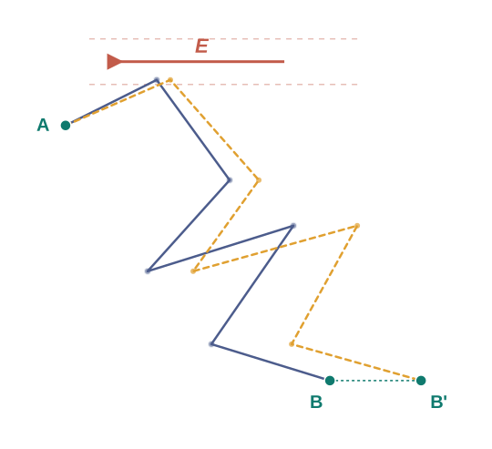
Fig. 3.4 – Electron path with and without an electric field.
Averaging over all electrons
The average velocity of all the electrons at time \(t\) is the average of all the \(\vec{V}_i\)’s. Look at the two terms in Eq. (3.16). The average of the \(\vec{v}_i\)’s is zero by Eq. (3.14), because right after any collision an electron’s direction is completely random.
The second term involves \(t_i\), the time since each electron’s last collision. These collisions do not happen at regular intervals but at random times, so at any instant some electrons have just collided (\(t_i\) small) while others have travelled freely for a while (\(t_i\) larger). Let us denote by \(\tau\) the average time between successive collisions — this is called the relaxation time. Averaging \(t_i\) over all the electrons gives \(\tau\).
Averaging Eq. (3.16) over all \(N\) electrons therefore gives the average velocity, which we call the drift velocity \(\vec{v}_d\): \[\vec{v}_d \equiv \left(\vec{V}_i\right)_{\text{average}} = \left(\vec{v}_i\right)_{\text{average}} - \frac{e\vec{E}}{m}\left(t_i\right)_{\text{average}}\] \[= 0 - \frac{e\vec{E}}{m}\tau = -\frac{e\vec{E}}{m}\tau \tag{3.17}\]
This result is surprising. Even though every electron is constantly being accelerated, their average velocity comes out to be a fixed value that does not grow with time. This steady average motion, superimposed on the random thermal jiggling, is called drift, and \(\vec{v}_d\) is the drift velocity.
From drift velocity to current
Because of this drift, there is now a net transport of charge across any area perpendicular to \(\vec{E}\). Consider a planar area \(A\) inside the conductor, with its normal parallel to \(\vec{E}\) (Fig. 3.5). In a very short time \(\Delta t\), every electron lying within a distance \(|\vec{v}_d|\Delta t\) to the left of the area will manage to cross it.
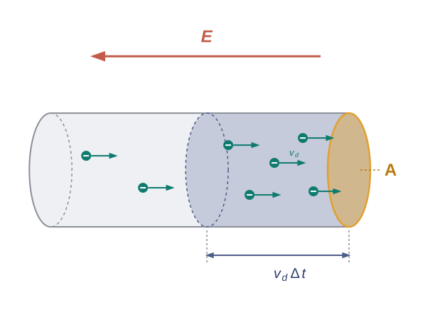
Fig. 3.5 – Charge crossing an area due to drift.
If \(n\) is the number of free electrons per unit volume (the number density), then the number of electrons in this crossing region is \(n\,\Delta t\,|\vec{v}_d|\,A\). Each electron carries charge \(-e\), so the total charge transported across the area to the right in time \(\Delta t\) is \(-neA|\vec{v}_d|\Delta t\). Since \(\vec{E}\) points to the left, the charge carried along \(\vec{E}\) is the negative of this — that is, a positive amount.
By the definition of current in Eq. (3.2), the amount of charge crossing area \(A\) in time \(\Delta t\) is \(I\,\Delta t\), where \(I\) is the magnitude of the current. Equating the two: \[I\,\Delta t = +\,n\,e\,A\,|\vec{v}_d|\,\Delta t \tag{3.18}\]
Now substitute the magnitude of the drift velocity from Eq. (3.17), \(|\vec{v}_d| = \dfrac{e|E|}{m}\tau\): \[I\Delta t = \frac{e^2 A}{m}\,\tau\,n\,\Delta t\,|E| \tag{3.19}\]
By definition, the current \(I\) is related to the magnitude \(|j|\) of the current density by \[I = |j|\,A \tag{3.20}\]
Combining Eqs. (3.19) and (3.20) — dividing through by \(A\,\Delta t\) — gives \[|j| = \frac{ne^2}{m}\,\tau\,|E| \tag{3.21}\]
The vector \(\vec{j}\) points along \(\vec{E}\), so we can write Eq. (3.21) in vector form: \[\vec{j} = \frac{ne^2}{m}\,\tau\,\vec{E} \tag{3.22}\]
Recovering Ohm’s law
Compare Eq. (3.22) with the form of Ohm’s law we met earlier, \(\vec{j} = \sigma\vec{E}\) [Eq. (3.13)]. They match exactly, provided we identify the conductivity \(\sigma\) as \[\sigma = \frac{ne^2}{m}\,\tau \tag{3.23}\]
This is a satisfying result: a very simple picture of electrons drifting and colliding reproduces Ohm’s law, and it even tells us what determines a material’s conductivity — the electron number density \(n\), the charge \(e\), the mass \(m\), and the relaxation time \(\tau\). Of course, we assumed that \(\tau\) and \(n\) are constants, independent of the field \(E\); in the next section we will discuss where Ohm’s law breaks down.
The comparison is striking: even in a wire carrying a few amperes, the electrons themselves only creep along at about a millimetre per second — slower than a snail. Yet a lamp lights up the instant you flip the switch. Example 3.2 explains how both can be true.
3.5.1 Mobility
We have just seen that conductivity comes from the presence of mobile charge carriers — charges free to drift under an electric field. It is worth pausing to note that these carriers are not always electrons. In metals the mobile carriers are electrons; in an ionised gas they are both electrons and positively charged ions; and in an electrolyte they can be both positive and negative ions. Whatever the carrier, the idea of drift under a field applies to all of them.
To compare how responsive different carriers are to a field, we introduce a useful quantity called mobility. Mobility, denoted by \(\mu\), is defined as the magnitude of the drift velocity produced per unit electric field: \[\mu = \frac{|\vec{v}_d|}{E} \tag{3.24}\]
Here \(|\vec{v}_d|\) is the magnitude of the drift velocity (in \(\text{m s}^{-1}\)) and \(E\) is the magnitude of the applied electric field (in \(\text{V m}^{-1}\)). In simple terms, mobility tells us how much drift speed a carrier picks up for a given “push” — a carrier with high mobility drifts quickly even in a modest field.
The SI unit of mobility is \(\text{m}^2/\text{Vs}\). In practical work, mobility is often quoted in the smaller units of \(\text{cm}^2/\text{Vs}\); a value expressed in the SI unit is \(10^4\) times the value expressed in these practical units. Note also that mobility is always taken as positive — it is defined using the magnitude of the drift velocity, so it does not depend on the sign of the carrier’s charge.
We can find a neat expression for mobility using our drift-velocity result. From Eq. (3.17), the magnitude of the drift velocity is \[v_d = \frac{e\tau E}{m}\]
Dividing by \(E\), as required by the definition in Eq. (3.24), the field cancels out: \[\mu = \frac{v_d}{E} = \frac{e\tau}{m} \tag{3.25}\]
where \(e\) is the magnitude of the carrier’s charge, \(m\) its mass, and \(\tau\) the average collision time (relaxation time) for the electrons.
This compact result is instructive. It shows that mobility depends only on the carrier itself and on how often it collides — not on the strength of the applied field. Carriers that are light (small \(m\)) or that go a long time between collisions (large \(\tau\)) have high mobility.
3.6 Limitations of Ohm’s Law
Ohm’s law is powerful and holds for a large class of materials — but it is not a universal law of nature. There are many materials and devices, widely used in real circuits, for which the simple proportionality between \(V\) and \(I\) breaks down. It is important to know how it can fail, because these failures are exactly what make devices like diodes useful.
The deviations from Ohm’s law fall broadly into one or more of the following three types.
Type (a): \(V\) is no longer proportional to \(I\).
For an ohmic conductor, a graph of \(V\) against \(I\) is a straight line through the origin — double the current and the voltage doubles too. In some materials this straight-line relationship holds only for small currents; beyond that, the graph bends. As shown in Fig. 3.6, the dashed line represents the ideal, linear Ohm’s-law behaviour, while the solid line shows the actual \(V\) versus \(I\) curve for such a conductor, which curves away from the straight line at larger values.
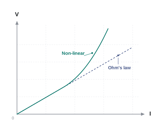
Fig. 3.6 – Non-linear V–I behaviour.
In this case the resistance is no longer a single fixed number — its effective value changes depending on how much current flows.
Type (b): the relation depends on the sign of \(V\).
For an ohmic conductor, reversing the applied voltage simply reverses the current, keeping its magnitude the same. But in some devices this symmetry is lost. If a certain voltage \(V\) produces a current \(I\), then reversing the direction of \(V\) while keeping its magnitude fixed does not produce a current of the same magnitude in the opposite direction.
A diode behaves exactly like this — you will study it in detail in Chapter 14. (A diode is a two-terminal electronic component that allows current to pass easily in one direction but strongly opposes it in the other.) Notice in Fig. 3.7 how the characteristic curve of a diode is very different on the two sides: the scales for positive and negative voltage and current are not even the same, because the device responds so differently depending on the direction of \(V\).
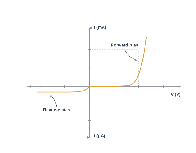
Fig. 3.7 – Characteristic curve of a diode.
Type (c): the relation is not unique.
For an ohmic conductor, each value of current corresponds to exactly one value of voltage. In some materials, however, the same current \(I\) can occur at more than one value of \(V\) — so the graph doubles back on itself. A material that shows this behaviour is gallium arsenide (GaAs).
As seen in Fig. 3.8, the current-versus-voltage curve for GaAs first rises, then enters a region where increasing the voltage actually decreases the current — a so-called negative resistance region — so that a single current value can be reached at several different voltages.
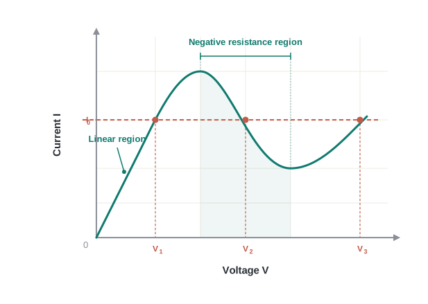
Fig. 3.8 – Current–voltage curve for GaAs.
Materials and devices that do not obey Ohm’s law in the form of Eq. (3.3) are, in fact, extremely common and useful in electronic circuits. Nevertheless, in this chapter and a few that follow, we will confine our study to materials that do obey Ohm’s law, since they let us build up the basic laws of circuits cleanly.
3.7 Resistivity of Various Materials
Different materials oppose the flow of current to very different degrees. Since resistivity \(\rho\) is the property that captures this opposition for a material (independent of its size or shape), it gives us a natural way to sort materials into groups. In fact, materials are classified as conductors, semiconductors, and insulators according to their resistivities, listed here in increasing order of their values.
Conductors have the lowest resistivities. Metals, in particular, have resistivities in the range of about \(10^{-8}\ \Omega\text{m}\) to \(10^{-6}\ \Omega\text{m}\). Because their resistivity is so small, they allow current to pass with very little opposition, which is why metals are used for wires and cables.
Insulators lie at the opposite extreme. Materials like ceramic, rubber, and plastics have resistivities that are around \(10^{18}\) times greater than those of metals, or even more. Such enormous resistivities mean these materials carry practically no current, which is why they are used to coat wires and to make protective casings.
Semiconductors fall in between the two. Their resistivities are much smaller than those of insulators but much larger than those of metals, placing them in the middle of the scale, as illustrated in Fig. 3.9.
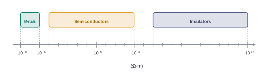
Fig. 3.9 – Resistivity ranges for different materials.
Semiconductors have a distinctive and very useful feature. Unlike metals, whose resistivity increases with temperature, semiconductors show a resistivity that characteristically decreases as the temperature is raised. (We will see the reason for this contrasting behaviour in the next section.)
There is a second, even more important way to change a semiconductor’s resistivity: its resistivity can be decreased by adding a small amount of a suitable impurity. This deliberate addition of impurities gives fine control over how well the material conducts.
3.8 Temperature Dependence of Resistivity
We noted in the last section that resistivity changes with temperature, and that metals and semiconductors respond in opposite ways. Here we make that quantitative for metals, and then explain the microscopic reason behind both behaviours.
The resistivity of a material depends on its temperature, and different materials do not respond in the same way. For a metallic conductor, over a range of temperatures that is not too large, the resistivity is approximately given by \[\rho_T = \rho_0\,[1 + \alpha\,(T - T_0)] \tag{3.26}\]
Here \(\rho_T\) is the resistivity at a temperature \(T\), and \(\rho_0\) is the resistivity at some chosen reference temperature \(T_0\). The quantity \(\alpha\) is called the temperature coefficient of resistivity.
From Eq. (3.26), \(\alpha\) measures the fractional change in resistivity per degree change in temperature. Its dimension is therefore \((\text{Temperature})^{-1}\), and its unit is \(^\circ\text{C}^{-1}\) (or \(\text{K}^{-1}\)). For metals, \(\alpha\) is positive, which means their resistivity rises as they get hotter.
Equation (3.26) is linear in \(T\), so a graph of \(\rho_T\) against \(T\) should be a straight line. For copper, this holds well over ordinary temperatures, as shown in Fig. 3.10 — but at temperatures much lower than \(0\,^\circ\text{C}\) the graph deviates considerably from a straight line, curving away.
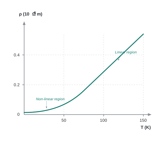
Fig. 3.10 – Resistivity of copper versus temperature.
For this reason, Eq. (3.26) is used only as an approximation over a limited range of \(T\) around a chosen reference temperature \(T_0\), where the graph can safely be treated as a straight line.
Materials with weak temperature dependence
Some materials show only a very weak change of resistivity with temperature. Nichrome — an alloy of nickel, iron, and chromium — is one such material, as seen in Fig. 3.11, where its resistivity changes only slightly across a wide temperature range. Manganin and constantan behave similarly.
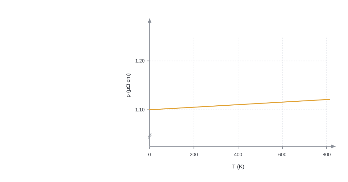
Fig. 3.11 – Resistivity of nichrome versus temperature.
Because their resistance barely shifts with temperature, these alloys are widely used to make wire-bound standard resistors — resistors whose values must stay reliable even as they warm up.
Semiconductors behave oppositely
Unlike metals, the resistivities of semiconductors decrease with increasing temperature. A typical semiconductor curve is shown in Fig. 3.12, where resistivity falls steeply as temperature rises.
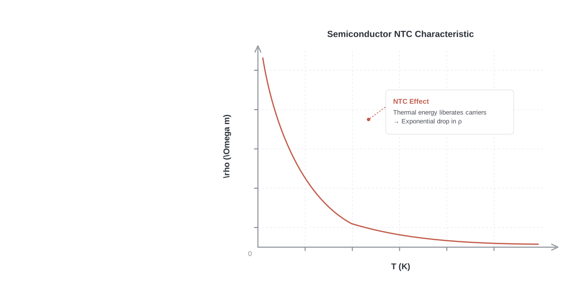
Fig. 3.12 – Resistivity of a semiconductor versus temperature.
Understanding it microscopically
We can understand all of this qualitatively using the result derived earlier for conductivity, Eq. (3.23). Taking its reciprocal, the resistivity of a material is \[\rho = \frac{1}{\sigma} = \frac{m}{n\,e^2\,\tau} \tag{3.27}\]
where \(m\) is the electron mass, \(e\) its charge magnitude, \(n\) the number of free carriers per unit volume, and \(\tau\) the average time between collisions. So \(\rho\) depends inversely on both \(n\) and \(\tau\): more carriers or fewer collisions means lower resistivity.
Now consider what heating does. As temperature rises, the carriers move faster on average, so they collide with the ions more often. This means the average collision time \(\tau\) decreases with temperature — an effect that, on its own, would raise the resistivity.
In a metal, the number of free electrons \(n\) hardly changes with temperature. So the only significant effect is the decrease in \(\tau\), and this causes the resistivity \(\rho\) to increase with temperature — exactly what we observe for metals.
For insulators and semiconductors, however, the number of carriers \(n\) increases strongly with temperature, because heat frees more charge carriers. This increase in \(n\) more than compensates for the decrease in \(\tau\) in Eq. (3.27), so for these materials the resistivity \(\rho\) decreases with temperature.
3.9 Electrical Energy, Power
A current flowing through a conductor does useful work — it lights bulbs, runs motors, and heats elements. But it also loses energy along the way. In this section we work out how much energy a current delivers and dissipates, and where that energy comes from.
Consider a conductor with two end points A and B, carrying a current \(I\) that flows from A to B. Let the electric potentials at these points be \(V(A)\) and \(V(B)\). Since the current flows from A to B, point A is at the higher potential, so \(V(A) > V(B)\), and the potential difference across AB is \[V = V(A) - V(B) > 0\]
In a time interval \(\Delta t\), an amount of charge \(\Delta Q = I\,\Delta t\) travels from A to B. By the definition of electric potential energy, the potential energy of this charge at A is \(\Delta Q\,V(A)\), and at B it is \(\Delta Q\,V(B)\). The change in its potential energy is therefore \[\Delta U_{\text{pot}} = \text{Final PE} - \text{Initial PE}\] \[= \Delta Q\,[V(B) - V(A)] = -\Delta Q\,V\] \[= -I\,V\,\Delta t < 0 \tag{3.28}\]
The negative sign tells us the charge loses potential energy as it moves from A to B — it “falls” through the potential difference, just as a stone loses gravitational potential energy falling downhill.
Where does that lost energy go?
If the charges moved through the conductor without any collisions, that lost potential energy would simply reappear as kinetic energy, keeping the total energy unchanged. Conservation of total energy would then give \[\Delta K = -\Delta U_{\text{pot}} \tag{3.29}\] that is, \[\Delta K = I\,V\,\Delta t > 0 \tag{3.30}\]
So, if charges moved freely under the field, they would keep speeding up, gaining kinetic energy as they go.
But we have already learned that this is not what happens. On average, the charge carriers do not accelerate — they move with a steady drift velocity. The reason is the collisions with the ions and atoms during their transit. At each collision, the energy that a charge has gained from the field is handed over to the atoms. The atoms then vibrate more vigorously, which is to say the conductor heats up.
So, in a real conductor, the energy that would have become kinetic energy is instead dissipated as heat. The amount of energy dissipated as heat during the time interval \(\Delta t\) is \[\Delta W = I\,V\,\Delta t \tag{3.31}\]
This is the microscopic answer to why a wire warms up: the electrons repeatedly give up their field-acquired energy to the lattice through collisions, and that shared energy shows up as heat.
Electric power
The energy dissipated per unit time is the power dissipated, \(P = \Delta W/\Delta t\). Dividing Eq. (3.31) by \(\Delta t\): \[P = I\,V \tag{3.32}\]
where \(P\) is the power (SI unit: watt, W), \(I\) is the current (A), and \(V\) is the potential difference (V).
Using Ohm’s law \(V = IR\), we can rewrite the power in two other useful forms: \[P = I^2 R = \frac{V^2}{R} \tag{3.33}\]
This is the power loss, often called ohmic loss or Joule heating, in a conductor of resistance \(R\) carrying current \(I\). It is exactly this power that heats the coil of an electric bulb until it glows white-hot, radiating out both heat and light.
Where does the power come from?
To keep a steady current flowing, we need an external source, as reasoned earlier. It is this source that must supply the dissipated power. In the simple circuit of Fig. 3.13, where a resistor \(R\) is connected across a cell, the power is supplied by the chemical energy stored in the cell — for as long as that chemical energy lasts.
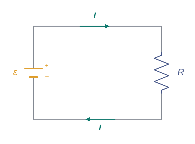
Fig. 3.13 – A simple circuit dissipating power.
The two expressions for power, Eqs. (3.32) and (3.33), show clearly how the power dissipated in a resistor depends on the current through it and the voltage across it.
Application to power transmission
Equation (3.33) has a hugely important application: the transmission of electrical power over long distances. Electrical power is sent from power stations to homes and factories, which may be hundreds of kilometres away, through long transmission cables. Naturally, we want to minimise the power wasted in these cables. Let us see how.
Suppose a device \(R\) is to receive a power \(P\), delivered through transmission cables that have their own resistance \(R_c\). If \(V\) is the voltage across the device and \(I\) the current through it, then the power delivered is \[P = V\,I \tag{3.34}\]
so the current needed to deliver this power is \(I = P/V\).
The connecting wires have a finite resistance \(R_c\), and the power dissipated (wasted) in them, \(P_c\), is the ohmic loss in that resistance: \[P_c = I^2 R_c\] Substituting \(I = P/V\): \[P_c = \frac{P^2 R_c}{V^2} \tag{3.35}\]
This is the key result. To deliver a fixed power \(P\) through cables of resistance \(R_c\), the power wasted in the wires is inversely proportional to \(V^2\). In other words, if we transmit at a higher voltage \(V\), the wasted power drops sharply — quadrupling the voltage cuts the loss to one-sixteenth.
Since real transmission cables run for hundreds of kilometres, their resistance \(R_c\) is considerable. To keep \(P_c\) small, these wires therefore carry electricity at enormous voltages — which is precisely why you see high-voltage danger signs on transmission lines running through the countryside.
Using electricity at such high voltages is not safe for household use, so at the receiving end a device called a transformer steps the voltage back down to a value suitable for homes and factories.
3.10 Cells, EMF, Internal Resistance
We have said several times that a steady current needs an external source to keep it going. The simplest such source is the electrolytic cell. In this section we look inside a cell to see how it maintains a current, and we meet two important quantities: the electromotive force (emf) and the internal resistance.
Basically, a cell has two electrodes — the positive electrode (P) and the negative electrode (N) — as shown in Fig. 3.14(a). Both are dipped in an electrolytic solution. Where each electrode meets the solution, it exchanges charges with the electrolyte, and this sets up potential differences right next to the electrodes.
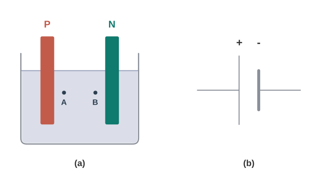
Fig. 3.14 – (a) An electrolytic cell and (b) its circuit symbol.
The positive electrode has a positive potential difference \(V_+\) (\(V_+ > 0\)) between itself and the electrolyte immediately next to it — this point in the solution is marked A in the figure. Likewise, the negative electrode develops a negative potential, written as \(-V_-\) (with \(V_- \geq 0\)), relative to the electrolyte next to it, marked B.
Defining the emf
When there is no current, the electrolyte has the same potential throughout, so the potential difference between the terminals P and N is the sum of these two contributions: \[V_+ - (-V_-) = V_+ + V_-\]
This open-circuit potential difference between the electrodes is called the electromotive force, or emf, of the cell, denoted by \(\varepsilon\): \[\varepsilon = V_+ + V_- > 0 \tag{3.36}\]
An important caution about the name: despite being called a “force,” the emf \(\varepsilon\) is actually a potential difference, measured in volts — not a force at all. The term is kept only for historical reasons, from a time when the phenomenon was not properly understood.
Connecting a load
To see the significance of \(\varepsilon\), connect a resistor \(R\) across the cell, as in Fig. 3.14. A current \(I\) then flows through \(R\) from C to D. A steady current is maintained because, inside the cell, the current flows from N to P through the electrolyte. So the same current \(I\) flows around the loop: from N to P through the electrolyte, and from P to N through the external resistor \(R\).
The electrolyte through which the current flows is not a perfect conductor — it has a finite resistance \(r\), called the internal resistance of the cell.
Open circuit: emf equals terminal potential difference.
First take the case when \(R\) is infinite, so no current flows (\(I = V/R = 0\)). Then the potential difference \(V\) between P and N is built up by adding the potential changes along the path from P through the electrolyte to N: \[V = (\text{PD between P and A}) + (\text{PD between A and B}) + (\text{PD between B and N}) = \varepsilon \tag{3.37}\]
With no current, the middle term (across the electrolyte) contributes nothing, and we simply recover \(V = \varepsilon\). This confirms that the emf is the terminal potential difference in an open circuit.
Closed circuit: terminal voltage drops.
If \(R\) is finite, then \(I\) is not zero, and some potential is now lost inside the cell across its internal resistance. The potential difference between P and N becomes \[V = V_+ + V_- - I r\] \[= \varepsilon - I r \tag{3.38}\]
The negative sign in the \(Ir\) term appears because, inside the electrolyte, the current flows from B to A, so there is a drop of potential \(Ir\) across the internal resistance. This quantity \(V = \varepsilon - Ir\) is the terminal voltage of the cell — the voltage actually available to the external circuit.
In practical calculations, the internal resistance can often be neglected when the current \(I\) is small enough that \(\varepsilon \gg Ir\). Actual internal resistances vary from cell to cell; notably, the internal resistance of a dry cell is much higher than that of a common (wet) electrolytic cell.
Finding the current in the circuit
Since \(V\) is also the potential difference across the external resistor \(R\), Ohm’s law gives \[V = I R \tag{3.39}\]
Combining Eqs. (3.38) and (3.39): \[I R = \varepsilon - I r\]
Bringing the \(Ir\) term to the left and solving for \(I\): \[I = \frac{\varepsilon}{R + r} \tag{3.40}\]
This neat result says the current is the emf divided by the total resistance of the circuit — external plus internal. The internal resistance \(r\) behaves just like an extra resistance in series with \(R\).
From Eq. (3.40), the maximum current that can be drawn from a cell occurs when \(R = 0\) (the terminals short-circuited), giving \[I_{\text{max}} = \frac{\varepsilon}{r}\]
In practice, however, the current allowed is kept well below this maximum, because such a large current would permanently damage the cell.
3.11 Cells in Series and in Parallel
Just as resistors can be combined and replaced by a single equivalent resistor, cells too can be combined in a circuit. And just like resistors, a combination of cells can be replaced — for the purpose of calculating currents and voltages — by a single equivalent cell. In this section we find the emf and internal resistance of that equivalent cell for two arrangements: series and parallel.
Cells in series
Consider first two cells connected in series (Fig. 3.15), where one terminal of one cell is joined to a terminal of the other, leaving the two outer terminals free. Let \(\varepsilon_1, \varepsilon_2\) be the emfs of the two cells and \(r_1, r_2\) their internal resistances.
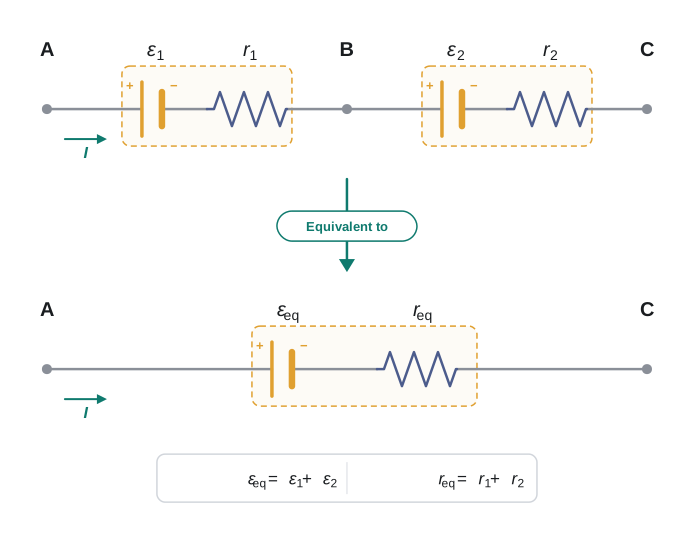
Fig. 3.15 – Two cells connected in series.
Let \(V(A)\), \(V(B)\), \(V(C)\) be the potentials at points A, B, and C in Fig. 3.15. Then \(V(A) - V(B)\) is the terminal potential difference of the first cell, which we already found in Eq. (3.38): \[V_{AB} \equiv V(A) - V(B) = \varepsilon_1 - I\,r_1 \tag{3.41}\]
Similarly, for the second cell, \[V_{BC} \equiv V(B) - V(C) = \varepsilon_2 - I\,r_2 \tag{3.42}\]
The potential difference across the whole combination, between A and C, is the sum of these: \[V_{AC} \equiv V(A) - V(C) = [V(A) - V(B)] + [V(B) - V(C)]\] \[= (\varepsilon_1 + \varepsilon_2) - I(r_1 + r_2) \tag{3.43}\]
Now suppose we replace the combination by a single equivalent cell between A and C, of emf \(\varepsilon_{eq}\) and internal resistance \(r_{eq}\). For that cell, \[V_{AC} = \varepsilon_{eq} - I\,r_{eq} \tag{3.44}\]
Comparing Eqs. (3.43) and (3.44) term by term gives \[\varepsilon_{eq} = \varepsilon_1 + \varepsilon_2 \tag{3.45}\] \[r_{eq} = r_1 + r_2 \tag{3.46}\]
So, for cells in series, the emfs add and the internal resistances add.
When a cell is reversed. In Fig. 3.15 we connected the negative electrode of the first cell to the positive electrode of the second. If instead the two negative electrodes are connected together, Eq. (3.42) changes sign to \(V_{BC} = -\varepsilon_2 - Ir_2\), and we obtain \[\varepsilon_{eq} = \varepsilon_1 - \varepsilon_2 \qquad (\varepsilon_1 > \varepsilon_2) \tag{3.47}\]
The rule extends to any number of cells in series:
Cells in parallel
Next consider a parallel combination of the two cells (Fig. 3.16). Let \(I_1\) and \(I_2\) be the currents leaving the positive electrodes of the two cells. At the point \(B_1\), currents \(I_1\) and \(I_2\) flow in, while the total current \(I\) flows out. Since charge is conserved (as much flows in as out), \[I = I_1 + I_2 \tag{3.48}\]
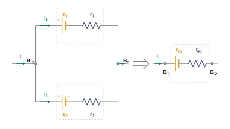
Fig. 3.16 – Two cells connected in parallel.
Let \(V(B_1)\) and \(V(B_2)\) be the potentials at \(B_1\) and \(B_2\). The terminal potential difference \(V = V(B_1) - V(B_2)\) is common to both cells (they are connected between the same two points). Applying Eq. (3.38) to the first cell, \[V \equiv V(B_1) - V(B_2) = \varepsilon_1 - I_1 r_1 \tag{3.49}\]
Since \(B_1\) and \(B_2\) are connected in exactly the same way to the second cell, \[V \equiv V(B_1) - V(B_2) = \varepsilon_2 - I_2 r_2 \tag{3.50}\]
From Eqs. (3.49) and (3.50), we can write \(I_1 = (\varepsilon_1 - V)/r_1\) and \(I_2 = (\varepsilon_2 - V)/r_2\). Substituting into Eq. (3.48): \[I = I_1 + I_2 = \frac{\varepsilon_1 - V}{r_1} + \frac{\varepsilon_2 - V}{r_2} = \left(\frac{\varepsilon_1}{r_1} + \frac{\varepsilon_2}{r_2}\right) - V\left(\frac{1}{r_1} + \frac{1}{r_2}\right) \tag{3.51}\]
Rearranging Eq. (3.51) to solve for \(V\): \[V = \frac{\varepsilon_1 r_2 + \varepsilon_2 r_1}{r_1 + r_2} - I\,\frac{r_1 r_2}{r_1 + r_2} \tag{3.52}\]
If we replace the combination by a single equivalent cell between \(B_1\) and \(B_2\), of emf \(\varepsilon_{eq}\) and internal resistance \(r_{eq}\), then \[V = \varepsilon_{eq} - I\,r_{eq} \tag{3.53}\]
Equations (3.52) and (3.53) must be identical, so comparing them gives \[\varepsilon_{eq} = \frac{\varepsilon_1 r_2 + \varepsilon_2 r_1}{r_1 + r_2} \tag{3.54}\] \[r_{eq} = \frac{r_1 r_2}{r_1 + r_2} \tag{3.55}\]
These can be put in a simpler, more symmetric form. Dividing appropriately, Eq. (3.55) becomes \[\frac{1}{r_{eq}} = \frac{1}{r_1} + \frac{1}{r_2} \tag{3.56}\] and Eq. (3.54) becomes \[\frac{\varepsilon_{eq}}{r_{eq}} = \frac{\varepsilon_1}{r_1} + \frac{\varepsilon_2}{r_2} \tag{3.57}\]
Notice that the internal resistances combine in parallel, exactly like resistors do.
When a cell is reversed. In Fig. 3.16 we joined the two positive terminals together and the two negative terminals together, so that \(I_1\) and \(I_2\) flow out of the positive terminals. If instead the negative terminal of the second cell is connected to the positive terminal of the first, Eqs. (3.56) and (3.57) still hold, but with \(\varepsilon_2 \to -\varepsilon_2\).
Extending to \(n\) cells. Equations (3.56) and (3.57) generalise easily. If \(n\) cells of emfs \(\varepsilon_1, \ldots, \varepsilon_n\) and internal resistances \(r_1, \ldots, r_n\) are connected in parallel, the combination is equivalent to a single cell of emf \(\varepsilon_{eq}\) and internal resistance \(r_{eq}\), such that \[\frac{1}{r_{eq}} = \frac{1}{r_1} + \cdots + \frac{1}{r_n} \tag{3.58}\] \[\frac{\varepsilon_{eq}}{r_{eq}} = \frac{\varepsilon_1}{r_1} + \cdots + \frac{\varepsilon_n}{r_n} \tag{3.59}\]
3.12 Kirchhoff’s Rules
Real electric circuits often contain many resistors and cells wired together in complicated ways. The series and parallel formulae we derived earlier are not always enough to find all the currents and voltages in such a network. For these cases we use two powerful rules, called Kirchhoff’s rules.
Before stating the rules, we need a clear way of labelling. Given a circuit, we assign to each resistor a current symbol, say \(I\), together with a directed arrow showing the assumed direction of flow. If the calculation finally gives \(I\) positive, the real current flows in the direction of the arrow; if \(I\) comes out negative, the real current flows opposite to the arrow. The arrow is just a guess — the sign of the answer corrects it.
For each source (a cell or other supply), we label the positive terminal P and the negative terminal N, and mark a current arrow. This lets us write the terminal potential difference. If the current \(I\) flows through the cell from N to P, then from Eq. (3.38), \[V = V(P) - V(N) = \varepsilon - I r\] If, while labelling, we instead take the current through the cell from P to N, then \[V = \varepsilon + I r \tag{3.60}\]
With the labelling clarified, we can now state the two rules.
(a) Junction rule
This applies not only at a junction where several wires meet, but at any point along a wire, as illustrated in Fig. 3.17.
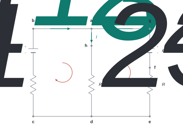
Fig. 3.17 – A network for Kirchhoff’s rules.
The reason behind the junction rule is charge conservation. When currents are steady, charge does not pile up anywhere — not at a junction, not at any point in a wire. So the rate at which charge flows into a junction (the incoming current) must exactly equal the rate at which it flows out (the outgoing current).
(b) Loop rule
The reason behind the loop rule is that electric potential has a definite value at each point. If we start at some point, travel around a closed loop, and return to the same point, we must return to the same potential — so the total change in potential around the loop adds up to zero.
The two worked examples below show the rules in action — first in a highly symmetric network, then in a general one where the full machinery is needed.
A battery of \(10\ \text{V}\) and negligible internal resistance is connected across the diagonally opposite corners of a cubical network made of \(12\) resistors, each of resistance \(1\ \Omega\) (Fig. 3.18). Find the equivalent resistance of the network and the current along each edge of the cube.
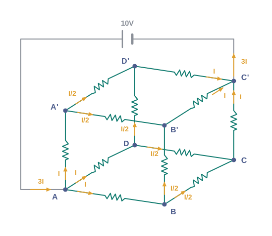
[Caption:] Fig. 3.18 – A cubical resistor network. [/Caption:]
Solution
This network cannot be reduced to simple series and parallel combinations. However, it has a clear symmetry we can exploit to find the equivalent resistance.
The three edges meeting at the input corner — AA′, AD, and AB — are placed symmetrically in the network, so the current in each must be the same, say \(I\). Then at the next corners (A′, B, and D), the incoming current \(I\) must split equally into the two outgoing branches, giving \(I/2\) in each. Continuing this way, and using the junction rule together with the symmetry, the current in all 12 edges can be written in terms of \(I\).
Now apply the loop rule (Kirchhoff’s second rule) to a closed loop, say ABCC′EA:
\[-IR - \frac{1}{2}IR - IR + \varepsilon = 0\]
where \(R\) is the resistance of each edge and \(\varepsilon\) is the emf of the battery. Solving,
\[\varepsilon = \frac{5}{2}IR\]
The equivalent resistance \(R_{eq}\) of the network relates \(\varepsilon\) to the total current, which is \(3I\) (the current supplied by the battery splits three ways at the input corner):
\[R_{eq} = \frac{\varepsilon}{3I} = \frac{5}{6}R\]
For \(R = 1\ \Omega\), this gives \(R_{eq} = \dfrac{5}{6}\ \Omega\). With \(\varepsilon = 10\ \text{V}\), the total current \((= 3I)\) in the network is
\[3I = \frac{10\ \text{V}}{(5/6)\ \Omega} = 12\ \text{A}, \quad \text{i.e., } I = 4\ \text{A}\]
The current in every edge can now be read off from Fig. 3.18 (each edge carries either \(I = 4\ \text{A}\) or \(I/2 = 2\ \text{A}\)).
Note that because of the network’s symmetry, the full power of Kirchhoff’s rules was not really needed here — the symmetry did most of the work. In a general network there is no such shortcut, and we must apply the rules to enough junctions and loops to solve for all unknowns. This is illustrated in the next example.
Determine the current in each branch of the network shown in Fig. 3.19.
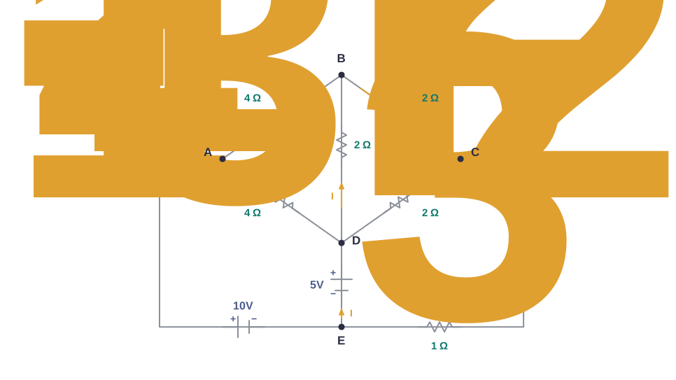
[Caption:] Fig. 3.19 – A bridge network with two cells. [/Caption:]
Solution
Each branch is assigned an unknown current. To keep the number of unknowns low from the start, we apply the junction rule at every junction, so that all branch currents are expressed in terms of just three unknowns \(I_1\), \(I_2\), and \(I_3\). These three are then found by applying the loop rule to three different closed loops.
Applying Kirchhoff’s loop rule to the closed loop ADCA:
\[10 - 4(I_1 - I_2) + 2(I_2 + I_3 - I_1) - I_1 = 0\]
which simplifies to
\[7I_1 - 6I_2 - 2I_3 = 10 \tag{3.61a}\]
For the closed loop ABCA:
\[10 - 4I_2 - 2(I_2 + I_3) - I_1 = 0\]
that is,
\[I_1 + 6I_2 + 2I_3 = 10 \tag{3.61b}\]
For the closed loop BCDEB:
\[5 - 2(I_2 + I_3) - 2(I_2 + I_3 - I_1) = 0\]
that is,
\[2I_1 - 4I_2 - 4I_3 = -5 \tag{3.61c}\]
Equations (3.61a), (3.61b), and (3.61c) are three simultaneous equations in three unknowns. Solving them by the usual method gives
\[I_1 = 2.5\ \text{A}, \quad I_2 = \frac{5}{8}\ \text{A}, \quad I_3 = 1\frac{7}{8}\ \text{A}\]
The currents in the various branches of the network are then
\[\text{AB}:\ \frac{5}{8}\ \text{A}, \quad \text{CA}:\ 2\frac{1}{2}\ \text{A}, \quad \text{DEB}:\ 1\frac{7}{8}\ \text{A}\]
\[\text{AD}:\ 1\frac{7}{8}\ \text{A}, \quad \text{CD}:\ 0\ \text{A}, \quad \text{BC}:\ 2\frac{1}{2}\ \text{A}\]
It is easily checked that applying Kirchhoff’s loop rule to the remaining loops gives no new independent equation — the values above satisfy the loop rule for every closed loop. For example, the total change in potential around the loop BADEB is
\[5\ \text{V} + \left(\frac{5}{8} \times 4\right)\text{V} - \left(\frac{15}{8} \times 4\right)\text{V}\]
which equals zero, as required by Kirchhoff’s loop rule.
3.13 Wheatstone Bridge
As a neat application of Kirchhoff’s rules, we now study a special circuit called the Wheatstone bridge. It is important not just as an exercise, but because it gives us a precise, practical way to measure an unknown resistance.
The Wheatstone bridge, shown in Fig. 3.20, is built from four resistors \(R_1\), \(R_2\), \(R_3\), and \(R_4\) arranged in a diamond shape. Across one pair of diagonally opposite corners (A and C in the figure) a source is connected; this diagonal AC is called the battery arm. Between the other two corners, B and D, a galvanometer G is connected. A galvanometer is a sensitive device that detects and measures small currents. This diagonal BD is called the galvanometer arm.
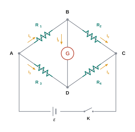
Fig. 3.20 – The Wheatstone bridge.
The balanced bridge
For simplicity, assume the cell has no internal resistance. In general, currents flow through all four resistors, and a current \(I_g\) flows through the galvanometer. The case of special interest is the balanced bridge, in which the four resistances are adjusted so that no current flows through the galvanometer, i.e. \(I_g = 0\). We now find the condition for this balance.
When \(I_g = 0\), applying Kirchhoff’s junction rule at junctions D and B immediately gives \[I_1 = I_3 \quad \text{and} \quad I_2 = I_4\] (because with no current diverted through G, whatever enters a junction along one arm must leave along the next).
Next, apply Kirchhoff’s loop rule to the two closed loops ADBA and CBDC. For the first loop (ADBA), with \(I_g = 0\): \[-I_1 R_1 + 0 + I_2 R_2 = 0 \tag{3.62}\] The “\(0\)” here is the potential change across the galvanometer, which is zero because no current flows through it.
For the second loop (CBDC), using \(I_3 = I_1\) and \(I_4 = I_2\): \[I_2 R_4 + 0 - I_1 R_3 = 0 \tag{3.63}\]
From Eq. (3.62), rearranging gives \[\frac{I_1}{I_2} = \frac{R_2}{R_1}\] and from Eq. (3.63), \[\frac{I_1}{I_2} = \frac{R_4}{R_3}\]
Since the left-hand sides are equal, the right-hand sides must be equal too, giving the balance condition: \[\frac{R_2}{R_1} = \frac{R_4}{R_3} \tag{3.64a}\]
Measuring an unknown resistance
The balance condition gives a practical method for finding an unknown resistance. Suppose the unknown resistance is placed in the fourth arm, so \(R_4\) is not known. Keeping known resistances \(R_1\) and \(R_2\) fixed in the first and second arms, we go on varying \(R_3\) until the galvanometer shows a null deflection. The bridge is then balanced, and from the balance condition the unknown resistance is \[R_4 = R_3 \frac{R_2}{R_1} \tag{3.64b}\]
A practical instrument built on this very principle is called the meter bridge.
The four arms of a Wheatstone bridge (Fig. 3.21) have the resistances \(\text{AB} = 100\ \Omega\), \(\text{BC} = 10\ \Omega\), \(\text{CD} = 5\ \Omega\), and \(\text{DA} = 60\ \Omega\). A galvanometer of \(15\ \Omega\) resistance is connected across BD. Calculate the current through the galvanometer when a potential difference of \(10\ \text{V}\) is maintained across AC.
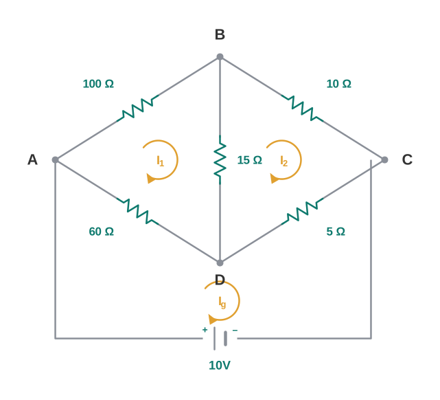
[Caption:] Fig. 3.21 – Calculating currents in a Wheatstone bridge. [/Caption:]
Solution
Here the bridge is not balanced, so a current \(I_g\) does flow through the galvanometer, and we must solve the circuit using Kirchhoff’s rules on three meshes.
Considering the mesh BADB:
\[100 I_1 + 15 I_g - 60 I_2 = 0\]
or, dividing through by 5,
\[20 I_1 + 3 I_g - 12 I_2 = 0 \tag{3.65a}\]
Considering the mesh BCDB:
\[10(I_1 - I_g) - 15 I_g - 5(I_2 + I_g) = 0\]
\[10 I_1 - 30 I_g - 5 I_2 = 0\]
which simplifies (dividing by 5) to
\[2 I_1 - 6 I_g - I_2 = 0 \tag{3.65b}\]
Considering the mesh ADCEA:
\[60 I_2 + 5(I_2 + I_g) = 10\]
\[65 I_2 + 5 I_g = 10\]
that is (dividing by 5),
\[13 I_2 + I_g = 2 \tag{3.65c}\]
Multiplying Eq. (3.65b) by 10:
\[20 I_1 - 60 I_g - 10 I_2 = 0 \tag{3.65d}\]
Subtracting Eq. (3.65a) from Eq. (3.65d) eliminates \(I_1\):
\[63 I_g - 2 I_2 = 0\]
\[I_2 = 31.5\, I_g \tag{3.65e}\]
Substituting the value of \(I_2\) from Eq. (3.65e) into Eq. (3.65c):
\[13(31.5\, I_g) + I_g = 2\]
\[410.5\, I_g = 2\]
\[I_g = 4.87\ \text{mA}\]
So a current of about \(4.87\ \text{mA}\) flows through the galvanometer — confirming the bridge is unbalanced, since the arm resistances do not satisfy the balance condition of Eq. (3.64a).
3.14 Summary
The current through a given area of a conductor is the net charge passing per unit time through that area.
To maintain a steady current, we need a closed circuit in which an external agency moves electric charge from lower to higher potential energy. The work done per unit charge by the source in carrying charge from lower to higher potential energy (that is, from one terminal of the source to the other) is called the electromotive force, or emf, of the source. Note that the emf is not a force; it is the potential difference between the two terminals of a source in an open circuit.
Ohm’s law: The electric current \(I\) flowing through a substance is proportional to the voltage \(V\) across its ends, i.e. \(V \propto I\) or \(V = RI\), where \(R\) is called the resistance of the substance. The unit of resistance is the ohm: \(1\ \Omega = 1\ \text{V A}^{-1}\).
The resistance \(R\) of a conductor depends on its length \(l\) and cross-sectional area \(A\) through the relation \[R = \frac{\rho l}{A}\] where \(\rho\), called the resistivity, is a property of the material and depends on temperature and pressure.
The electrical resistivity of substances spans a very wide range. Metals have low resistivity, in the range of \(10^{-8}\ \Omega\text{m}\) to \(10^{-6}\ \Omega\text{m}\). Insulators like glass and rubber have resistivity \(10^{22}\) to \(10^{24}\) times greater. Semiconductors like Si and Ge lie roughly in the middle range of resistivity on a logarithmic scale.
In most substances the carriers of current are electrons; in some cases — for example, ionic crystals and electrolytic liquids — positive and negative ions carry the electric current.
Current density \(\vec{j}\) gives the amount of charge flowing per second per unit area normal to the flow: \[\vec{j} = nq\,\vec{v}_d\] where \(n\) is the number density (number per unit volume) of charge carriers, each of charge \(q\), and \(\vec{v}_d\) is the drift velocity of the carriers. For electrons, \(q = -e\). If \(\vec{j}\) is normal to a cross-sectional area \(A\) and is constant over the area, the magnitude of the current \(I\) through the area is \(n e v_d A\).
Using \(E = V/l\), \(I = n e v_d A\), and Ohm’s law, one obtains \[\frac{eE}{m} = \rho\,\frac{ne^2}{m}\,v_d\] The proportionality between the force \(eE\) on the electrons (due to the external field \(E\)) and the drift velocity \(v_d\) — rather than the acceleration — can be understood if we assume the electrons suffer collisions with ions in the metal that deflect them randomly. If such collisions occur on average at a time interval \(\tau\), \[v_d = a\tau = eE\tau/m\] where \(a\) is the acceleration of the electron. This gives \[\rho = \frac{m}{ne^2\tau}\]
In the temperature range where resistivity increases linearly with temperature, the temperature coefficient of resistivity \(\alpha\) is defined as the fractional increase in resistivity per unit increase in temperature.
Ohm’s law is obeyed by many substances, but it is not a fundamental law of nature. It fails if:
- \(V\) depends on \(I\) non-linearly;
- the relation between \(V\) and \(I\) depends on the sign of \(V\) for the same absolute value of \(V\);
- the relation between \(V\) and \(I\) is non-unique. An example of (a) is when \(\rho\) increases with \(I\) (even at fixed temperature). A rectifier combines features (a) and (b). GaAs shows feature (c).
When a source of emf \(\varepsilon\) is connected to an external resistance \(R\), the voltage \(V_{\text{ext}}\) across \(R\) is given by \[V_{\text{ext}} = IR = \frac{\varepsilon}{R + r}\,R\] where \(r\) is the internal resistance of the source.
Kirchhoff’s Rules:
- Junction Rule: At any junction of circuit elements, the sum of the currents entering the junction must equal the sum of the currents leaving it.
- Loop Rule: The algebraic sum of changes in potential around any closed loop must be zero.
- The Wheatstone bridge is an arrangement of four resistances \(R_1, R_2, R_3, R_4\) as shown in the text. Its null-point (balance) condition is given by \[\frac{R_1}{R_2} = \frac{R_3}{R_4}\] using which the value of one resistance can be determined, knowing the other three.
Reference table of physical quantities
| Physical Quantity | Symbol | Dimensions | Unit | Remark |
|---|---|---|---|---|
| Electric current | \(I\) | \([\text{A}]\) | A | SI base unit |
| Charge | \(Q,\ q\) | \([\text{T A}]\) | C | |
| Voltage, Electric potential difference | \(V\) | \([\text{M L}^2\text{T}^{-3}\text{A}^{-1}]\) | V | Work/charge |
| Electromotive force | \(\varepsilon\) | \([\text{M L}^2\text{T}^{-3}\text{A}^{-1}]\) | V | Work/charge |
| Resistance | \(R\) | \([\text{M L}^2\text{T}^{-3}\text{A}^{-2}]\) | \(\Omega\) | \(R = V/I\) |
| Resistivity | \(\rho\) | \([\text{M L}^3\text{T}^{-3}\text{A}^{-2}]\) | \(\Omega\,\text{m}\) | \(R = \rho l/A\) |
| Electrical conductivity | \(\sigma\) | \([\text{M}^{-1}\text{L}^{-3}\text{T}^{3}\text{A}^{2}]\) | S | \(\sigma = 1/\rho\) |
| Electric field | \(\vec{E}\) | \([\text{M L T}^{-3}\text{A}^{-1}]\) | \(\text{V m}^{-1}\) | Electric force / charge |
| Drift speed | \(v_d\) | \([\text{L T}^{-1}]\) | \(\text{m s}^{-1}\) | \(v_d = \dfrac{eE\tau}{m}\) |
| Relaxation time | \(\tau\) | \([\text{T}]\) | s | |
| Current density | \(\vec{j}\) | \([\text{L}^{-2}\text{A}]\) | \(\text{A m}^{-2}\) | current/area |
| Mobility | \(\mu\) | \([\text{M}^{-1}\text{L}^{0}\text{T}^{2}\text{A}]\) | \(\text{m}^2\text{V}^{-1}\text{s}^{-1}\) | \(v_d/E\) |
3.15 Points to Ponder
Current is a scalar, even though we draw it with an arrow. The arrow only shows the direction of flow along a wire; it does not make current a vector. Currents do not obey the law of vector addition — if two wires carrying currents meet, the currents do not add like vectors. That current is a scalar also follows from its definition: the current \(I\) through an area of cross-section is the scalar (dot) product of two vectors, \[I = \vec{j} \cdot \Delta\vec{S}\] where the current density \(\vec{j}\) and the area element \(\Delta\vec{S}\) are both vectors, but their dot product \(I\) is a scalar.
\(V = IR\) is not, by itself, a statement of Ohm’s law. Look again at the \(V\)–\(I\) curves of a resistor and a diode drawn in the text: a resistor obeys Ohm’s law, but a diode does not. The equation \(V = IR\) simply defines resistance, and it can be applied to any conducting device — whether or not it obeys Ohm’s law. What Ohm’s law actually asserts is stronger: that the plot of \(I\) against \(V\) is a straight line, i.e. that \(R\) is independent of \(V\). The relation \(\vec{E} = \rho\vec{j}\) leads to an equivalent statement of Ohm’s law: a conducting material obeys Ohm’s law when its resistivity does not depend on the magnitude or direction of the applied electric field.
Even “ohmic” materials obey Ohm’s law only within a range. Homogeneous conductors like silver, or semiconductors like pure germanium (or germanium with impurities), obey Ohm’s law only within a certain range of electric field values. If the field becomes too strong, departures from Ohm’s law appear in all cases.
Only the field-driven part of the electron’s motion produces drift. The motion of a conduction electron in a field \(\vec{E}\) is the sum of two parts: (i) motion due to random collisions, and (ii) motion due to the field \(\vec{E}\). The part due to random collisions averages to zero and contributes nothing to the drift velocity \(v_d\) (as discussed in the Class XI textbook). Thus \(v_d\) arises solely from the applied electric field acting on the electron.
The relation \(\vec{j} = \rho\vec{v}\) must be applied to each type of charge carrier separately. (Here \(\rho\) denotes the charge density, not resistivity.) In a conducting wire, the total current and charge density come from both positive and negative charges: \[\vec{j} = \rho_+\vec{v}_+ + \rho_-\vec{v}_-\] \[\rho = \rho_+ + \rho_-\] Now, in a neutral wire carrying a current, the positive and negative charge densities cancel: \[\rho_+ = -\rho_-\] Also, the positive ions are essentially fixed, so \(v_+ \approx 0\), which gives \[\rho = 0\] \[\vec{j} = \rho_-\vec{v}\] So, although the wire carries a current, its total charge density is zero — and therefore the relation \(\vec{j} = \rho\vec{v}\) does not apply to the total current and total charge density; it must be used carrier by carrier.
Kirchhoff’s junction rule rests on conservation of charge. The outgoing currents at a junction add up to equal the incoming current, because charge cannot accumulate there in the steady state. Bending or reorienting the wire makes no difference — it does not change the validity of the junction rule.
3.16 NCERT Questions
The storage battery of a car has an emf of \(12\ \text{V}\). If the internal resistance of the battery is \(0.4\ \Omega\), what is the maximum current that can be drawn from the battery?
A battery of emf \(10\ \text{V}\) and internal resistance \(3\ \Omega\) is connected to a resistor. If the current in the circuit is \(0.5\ \text{A}\), what is the resistance of the resistor? What is the terminal voltage of the battery when the circuit is closed?
At room temperature (\(27.0\ ^\circ\text{C}\)) the resistance of a heating element is \(100\ \Omega\). What is the temperature of the element if the resistance is found to be \(117\ \Omega\), given that the temperature coefficient of the material of the resistor is \(1.70 \times 10^{-4}\ ^\circ\text{C}^{-1}\)?
A negligibly small current is passed through a wire of length \(15\ \text{m}\) and uniform cross-section \(6.0 \times 10^{-7}\ \text{m}^2\), and its resistance is measured to be \(5.0\ \Omega\). What is the resistivity of the material at the temperature of the experiment?
A silver wire has a resistance of \(2.1\ \Omega\) at \(27.5\ ^\circ\text{C}\), and a resistance of \(2.7\ \Omega\) at \(100\ ^\circ\text{C}\). Determine the temperature coefficient of resistivity of silver.
A heating element using nichrome connected to a \(230\ \text{V}\) supply draws an initial current of \(3.2\ \text{A}\), which settles after a few seconds to a steady value of \(2.8\ \text{A}\). What is the steady temperature of the heating element if the room temperature is \(27.0\ ^\circ\text{C}\)? The temperature coefficient of resistance of nichrome averaged over the temperature range involved is \(1.70 \times 10^{-4}\ ^\circ\text{C}^{-1}\).
Determine the current in each branch of the network shown in Fig. 3.22.
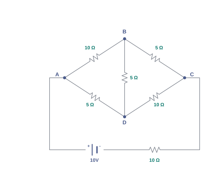
Fig. 3.22 – Bridge network for branch currents.
A storage battery of emf \(8.0\ \text{V}\) and internal resistance \(0.5\ \Omega\) is being charged by a \(120\ \text{V}\) dc supply using a series resistor of \(15.5\ \Omega\). What is the terminal voltage of the battery during charging? What is the purpose of having a series resistor in the charging circuit?
The number density of free electrons in a copper conductor, estimated in Example 3.1, is \(8.5 \times 10^{28}\ \text{m}^{-3}\). How long does an electron take to drift from one end of a wire \(3.0\ \text{m}\) long to its other end? The area of cross-section of the wire is \(2.0 \times 10^{-6}\ \text{m}^2\) and it is carrying a current of \(3.0\ \text{A}\).
3.17 Check Your Concepts
Current has a direction of flow associated with it, yet it is classified as a scalar quantity. Explain why current is a scalar and not a vector.
The drift speed of electrons in a copper wire is only about a millimetre per second, yet an electric lamp lights up almost the instant its switch is closed. Explain how both statements can be true at the same time.
Using the relation \(\rho = \dfrac{m}{ne^2\tau}\), explain why the resistivity of a metal increases with temperature while that of a semiconductor decreases with temperature.
The terminal voltage of a cell equals its emf in an open circuit but is smaller than the emf when the cell drives a current. Explain the reason for this difference.
Electrical power is transmitted over long distances at very high voltages, even though such voltages are dangerous. Using the expression for power loss in the transmission line, justify this choice.
A diode does not obey Ohm’s law. Does this mean the relation \(R = V/I\) cannot be applied to it? Distinguish clearly between the equation \(V = IR\) as a definition of resistance and Ohm’s law.
State the conservation principle on which each of Kirchhoff’s two rules is based, and explain briefly how each principle leads to its rule.
In measuring an unknown resistance with a Wheatstone bridge, why is a null (zero-deflection) reading of the galvanometer preferred over reading a non-zero deflection?
Assertion: Connecting several identical cells in parallel increases the maximum current that can be drawn from the combination. Reason: The equivalent internal resistance of cells in parallel is smaller than that of a single cell. Evaluate whether the assertion and the reason are correct, and whether the reason correctly explains the assertion.
Alloys such as nichrome, manganin, and constantan are used to make standard resistors and heating elements. Which specific property of these alloys makes them suitable for these uses, and why?
3.18 Practice with Numericals
A steady current of \(2.0\ \text{A}\) flows through a conductor. How many electrons cross a given cross-section of the conductor in one minute? (Take \(e = 1.6 \times 10^{-19}\ \text{C}\).)
A copper wire has a length of \(5.0\ \text{m}\) and a uniform cross-sectional area of \(2.0 \times 10^{-7}\ \text{m}^2\). If the resistivity of copper is \(1.7 \times 10^{-8}\ \Omega\text{m}\), calculate the resistance of the wire.
A wire of cross-sectional area \(2.0 \times 10^{-6}\ \text{m}^2\) carries a current of \(5.0\ \text{A}\). If the number density of free electrons is \(8.5 \times 10^{28}\ \text{m}^{-3}\), estimate the drift speed of the electrons. (Take \(e = 1.6 \times 10^{-19}\ \text{C}\).)
A metallic wire of resistance \(4\ \Omega\) is stretched uniformly until its length is doubled, its volume remaining unchanged. Find the new resistance of the wire.
The resistance of a metal coil is \(20\ \Omega\) at \(0\ ^\circ\text{C}\). If the temperature coefficient of resistance of the metal is \(5.0 \times 10^{-3}\ ^\circ\text{C}^{-1}\), find the resistance of the coil at \(50\ ^\circ\text{C}\) (assume the dimensions do not change appreciably).
An electric heater is rated \(1000\ \text{W}\) at \(220\ \text{V}\). Calculate (a) the resistance of its element and (b) the current it draws. (c) How much electrical energy, in kilowatt-hours, does it consume if used for \(2\) hours?
A cell of emf \(1.5\ \text{V}\) and internal resistance \(0.5\ \Omega\) is connected across an external resistance of \(2.5\ \Omega\). Find (a) the current in the circuit, (b) the terminal voltage of the cell, and (c) the power dissipated in the external resistance.
Three identical cells, each of emf \(2.0\ \text{V}\) and internal resistance \(0.2\ \Omega\), are connected in series (all aiding) across an external resistance of \(4.4\ \Omega\). Calculate the current in the circuit.
In a balanced Wheatstone bridge, three of the four arms have resistances \(R_1 = 10\ \Omega\), \(R_2 = 20\ \Omega\), and \(R_3 = 15\ \Omega\), arranged so that the balance condition is \(\dfrac{R_2}{R_1} = \dfrac{R_4}{R_3}\). Determine the value of the fourth resistance \(R_4\).
In a certain conductor, the electrons acquire a drift speed of \(2.5 \times 10^{-4}\ \text{m s}^{-1}\) when an electric field of magnitude \(0.5\ \text{V m}^{-1}\) is applied. Calculate the mobility of the electrons.