Chapter 10: Wave Optics
In the year 1801, an English scientist named Thomas Young set up an experiment so simple that anyone could repeat it, yet its result shook the science of his time. He let light from a single bright source fall on a screen that had two tiny, closely spaced pinholes cut into it. The light passing through these two holes then landed on a second screen behind them.
By common sense, one would expect two overlapping patches of light — brighter where they overlapped, and nothing unusual otherwise. But that is not what Young saw. Instead, the second screen showed a neat pattern of alternating bright and dark bands, one after another. In some places, light added to light and grew brighter; in other places, light added to light and produced complete darkness.
This was startling. If light were made of tiny particles, as the great Isaac Newton had argued, two streams of particles could never cancel each other to give darkness. But if light were a wave, like ripples on water, then two waves meeting crest-to-trough could indeed cancel out. Young’s bands were direct evidence that light is a wave. Against the weight of Newton’s authority, this experiment slowly turned the tide of physics.
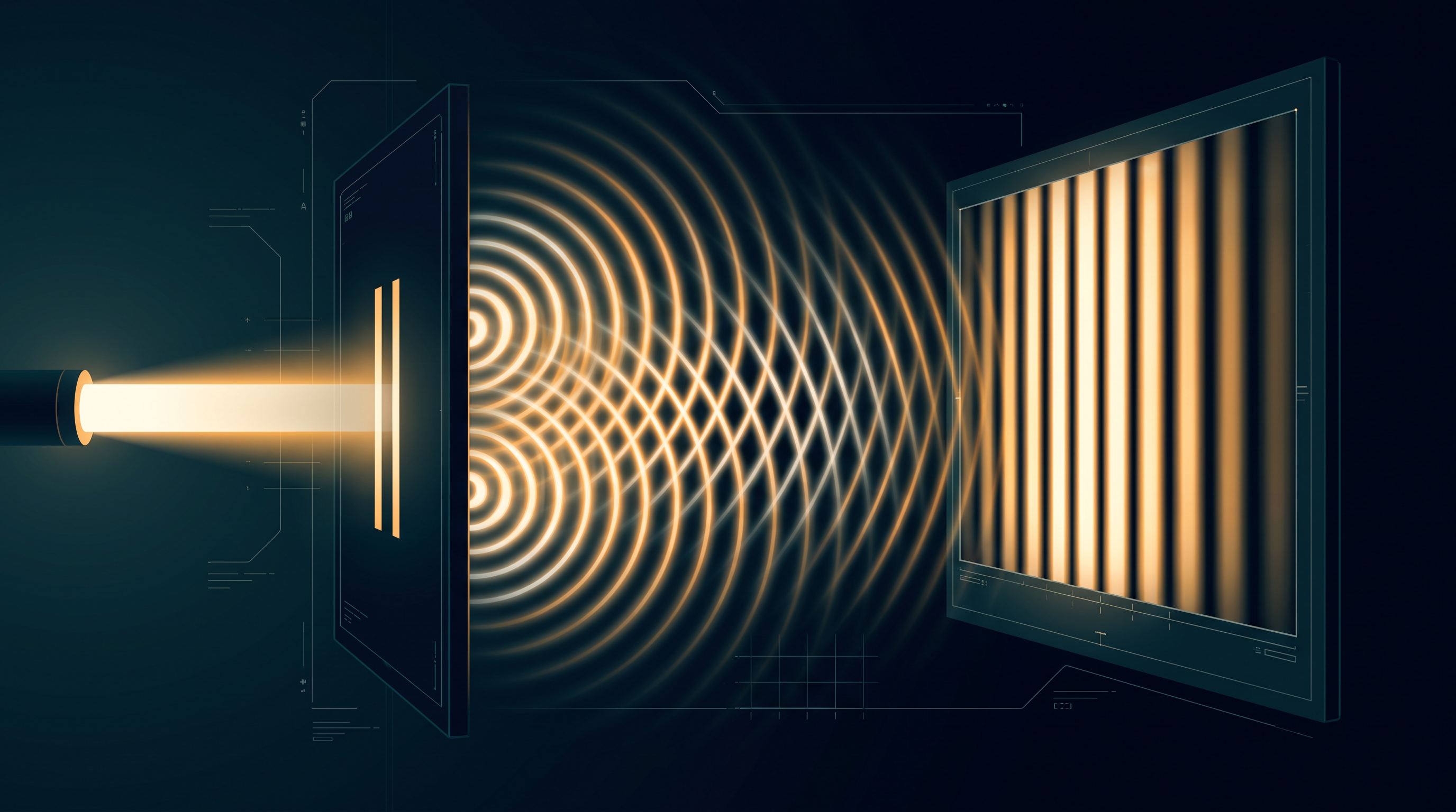
Fig. 10.0 – Young’s double-slit experiment.
By the end of this chapter, you will be able to answer each of these questions using the wave model of light.
10.1 Introduction
For a long time, one of the deepest questions in physics was surprisingly basic: what exactly is light? Over the centuries, two very different pictures competed to answer this, and the contest between them shaped the whole of optics.
The first picture was the corpuscular model. The word “corpuscle” simply means a tiny particle, so this model imagined light as a stream of extremely small particles shot out from a source, much like a spray of tiny bullets. In 1637 the French thinker Descartes used this particle idea to derive Snell’s law, the rule you already know that describes how a ray bends when it passes from one medium into another. The corpuscular model successfully explained both the laws of reflection (how light bounces off a surface) and the laws of refraction (how light bends at the boundary between two media).
This particle model was later developed further by Isaac Newton in his famous book OPTICKS. Because that book was so widely read and admired, the corpuscular model of light came to be linked mainly with Newton’s name.
There was, however, one sharp prediction hidden inside the corpuscular model. It predicted that when a ray of light bends towards the normal on entering a second medium (as it does when going from air into water or glass), the speed of light must become greater in that second medium. Remember this prediction — it is the point on which the whole particle-versus-wave debate would eventually be decided.
The second picture was the wave model. In 1678 the Dutch physicist Christiaan Huygens put forward the idea that light travels as a wave, spreading out much like ripples on the surface of a pond. It is this wave model of light that we will study throughout this chapter. The wave model could also explain reflection and refraction perfectly well — but it made exactly the opposite prediction about speed. According to the wave model, when light bends towards the normal on entering a denser medium, its speed must become less in that medium, not greater.
Here, then, was a clean way to test the two rival models against each other.
The answer came much later. Careful experiments showed that the speed of light in water is actually less than the speed of light in air. This matched the wave model’s prediction and directly contradicted the corpuscular model’s. The French physicist Foucault carried out this decisive measurement in 1850. Light, it turned out, slows down when it enters a denser medium.
So light behaves as a wave, and it slows down (rather than speeds up) in a denser medium such as water or glass. This settles the two halves of our opening question — even though, as we will see in Section 10.3, the full geometric reasoning behind why the speed decreases comes from Huygens’ own construction.
Interestingly, the wave theory was not readily accepted at first. There were two reasons. One was simply the enormous authority of Newton, which made scientists reluctant to abandon his particle picture. The other was a genuine physical puzzle: light can travel through empty space (a vacuum), yet at that time people believed that any wave must have a material medium to travel through. A wave with nothing to wave in seemed impossible.
The turning point came when Thomas Young performed his famous interference experiment in 1801 — the same experiment described at the start of this chapter. Its bright-and-dark banded pattern could only be explained if light were a wave, and this firmly established the wave nature of light.
Once light was accepted as a wave, its wavelength could be measured, and it was found to be extremely small. For example, the wavelength of yellow light is only about \(0.6\ \mu\text{m}\) (that is, \(0.6\) millionths of a metre). This smallness has an important consequence. Compared to the size of ordinary mirrors and lenses, the wavelength of visible light is tiny, so light can be treated, to a very good approximation, as travelling in perfectly straight lines. This straight-line treatment is exactly the field of geometrical optics that you studied in the previous chapter.
After Young’s experiment of 1801, for the next forty years or so many further experiments were carried out on the interference and diffraction of light waves. These could be satisfactorily explained only by assuming a wave model. As a result, by around the middle of the nineteenth century the wave theory of light seemed very firmly established.
Yet the old puzzle still remained: if a wave needs a medium, how can light waves cross a vacuum? This was finally explained when James Clerk Maxwell put forward his electromagnetic theory of light. Maxwell had assembled a set of equations describing all the known laws of electricity and magnetism. From these equations he derived a wave equation, and from it he predicted the existence of electromagnetic waves.
Using that wave equation, Maxwell could even calculate the speed of electromagnetic waves in free space. Remarkably, the value he obtained came out very close to the already-measured speed of light. From this striking match, Maxwell boldly concluded that light must be an electromagnetic wave.
This idea also solved the vacuum puzzle. According to Maxwell, a light wave is a partnership of changing electric and magnetic fields: a changing electric field produces a magnetic field that varies in both space and time, and a changing magnetic field in turn produces a similarly varying electric field. Each field keeps regenerating the other. Because these fields do not need any material to exist in, this self-sustaining electric–magnetic disturbance can travel even through a vacuum — which is exactly how sunlight reaches us across empty space.
As you study these historical predictions, note a point that examiners are fond of: the corpuscular and wave models agreed on the observations (reflection and refraction) but disagreed on the speed of light in a denser medium. Questions of the “which model predicts what, and which experiment decided it” type are common in the conceptual and assertion–reason sections of board and competitive exams.
Here is the plan for the rest of the chapter. We will first discuss the original formulation of the Huygens principle and use it to derive the laws of reflection and refraction. In Sections 10.4 and 10.5 we will study the phenomenon of interference, which rests on the principle of superposition. In Section 10.6 we will study diffraction, which is based on the Huygens–Fresnel principle. Finally, in Section 10.7 we will study polarisation, a phenomenon that depends on the fact that light waves are transverse electromagnetic waves.
10.2 Huygens Principle
To study light as a wave, we first need a clear way of picturing a wave as it spreads. That picture is built around a single powerful idea called the wavefront. Let us build it up from a familiar scene.
Imagine dropping a small stone into a calm pool of water. Waves spread outward from the point where the stone struck. Every point on the water surface begins to bob up and down (oscillate) as the disturbance reaches it.
Now suppose we could take an instant photograph of the surface. We would see a set of circular rings — the crests — marking the places where the disturbance is at our maximum at that instant. Every point sitting on one such circle is at the same distance from the source, so all these points are moving up and down together, in step. Points moving in step like this are said to be in phase.
Such a set of points, all oscillating in phase, is what we call a wavefront.
The wavefront does not sit still; it moves steadily outward from the source. The rate at which it advances is exactly what we mean by the speed of the wave. And importantly, the energy of the wave is carried in the direction perpendicular to the wavefront — that perpendicular direction is precisely the “ray” we defined in the previous section. This is the key link between the wave picture and the ray picture: rays always run at right angles to wavefronts.
Now consider the shape of a wavefront. If a point source sends out waves equally in all directions, then the points that share the same amplitude and the same phase lie on the surface of a sphere. This gives a spherical wave, whose wavefronts are spheres growing outward, as shown in Fig. 10.1(a).
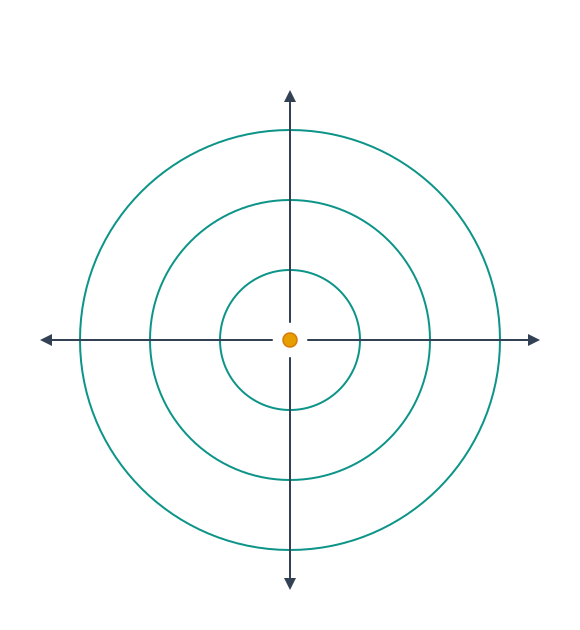
Fig. 10.1(a) – Spherical wavefront from a point source.
If we move very far away from the source, the sphere becomes so large that any small patch of it looks almost flat — in the same way that a small patch of the (curved) Earth looks flat to us standing on it. Such a nearly flat wavefront is called a plane wave, shown in Fig. 10.1(b).
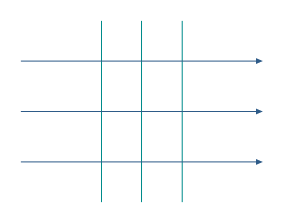
Fig. 10.1(b) – Plane wavefront.
We now arrive at the central question of this section — and one of the opening questions of the chapter. Suppose we know the exact shape of a wavefront right now, at time \(t = 0\). Can we predict where the wavefront will be at some later time? Huygens gave a beautifully simple geometrical recipe to do exactly this.
Let us apply it to a diverging (spreading) wave. Let \(F_1F_2\) represent a portion of a spherical wavefront at \(t = 0\), as shown in Fig. 10.2. Huygens’ idea is this: treat every single point on this wavefront as though it were itself a tiny new source. Each such point sends out its own little wavelets, called secondary wavelets, which spread out in all directions with the speed of the wave.
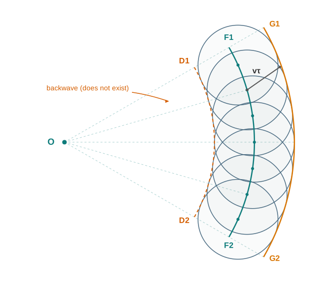
Fig. 10.2 – Huygens’ geometrical construction for a spherical wave.
Let us see the construction in detail. Suppose we want the wavefront after a time interval \(\tau\). In that time, each secondary wavelet travels a distance equal to (speed × time), that is \(v\tau\), where \(v\) is the speed of the wave in the medium (in metres per second, \(\text{m s}^{-1}\)) and \(\tau\) is the time interval (in seconds, \(\text{s}\)).
So from each point of the original wavefront \(F_1F_2\), we draw a small sphere of radius \(v\tau\). When we draw the surface that just touches all these little spheres on the forward side — their common tangent — we obtain the new wavefront, shown as \(G_1G_2\) in Fig. 10.2. For a spherical wave, this new wavefront \(G_1G_2\) is again a sphere with the same centre \(O\), simply of a larger radius. The wave has advanced, keeping its spherical shape.
There is, however, a hitch in this simple picture. Since each point sends wavelets out in all directions, drawing common tangents should give not only a forward wavefront but also a backward one — a “backwave,” marked \(D_1D_2\) in Fig. 10.2. But no such backward-travelling wave is ever actually seen.
Huygens dealt with this by assuming that the amplitude of the secondary wavelets is maximum in the forward direction and zero in the backward direction. With that assumption, the backwave simply vanishes. It must be said honestly that this was an ad hoc assumption — a patch introduced just to fit the observation. The real justification for the absence of the backwave comes only from more rigorous wave theory developed later.
The same construction works just as well for a plane wave travelling through a medium, as shown in Fig. 10.3. Here the flat wavefront \(F_1F_2\) at \(t = 0\) advances to a new flat wavefront \(G_1G_2\) at a later time \(\tau\), again found as the common tangent to the secondary wavelets. The straight lines \(A_1A_2\), \(B_1B_2\), and so on are drawn perpendicular (“normal”) to both \(F_1F_2\) and \(G_1G_2\); these perpendicular lines are exactly the rays of the wave, showing once more how rays and wavefronts always meet at right angles.
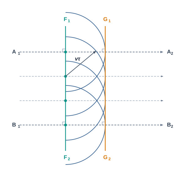
Fig. 10.3 – Huygens’ construction for a plane wave.
In exams, this section is most often tested by asking you to sketch the shape of a wavefront in a given situation (from a point source, from a very distant star, or after passing through a lens or mirror) and to recall that rays are always perpendicular to wavefronts. Keeping the wavefront-and-ray relationship firmly in mind makes such questions straightforward.
10.3 Refraction and Reflection of Plane Waves using Huygens Principle
10.3.1 Refraction of a plane wave
In the previous section we learned Huygens’ recipe for advancing a wavefront. We will now put that recipe to work and use it to derive the laws of refraction — the rules that govern how light bends when it crosses from one medium into another. This is a good example of how a wave picture can reproduce, and even explain, the ray-optics laws you already know.
Let \(PP'\) be the flat surface separating two media, called medium 1 (above) and medium 2 (below), as shown in Fig. 10.4. Let \(v_1\) and \(v_2\) be the speeds of light in medium 1 and medium 2 respectively, each measured in metres per second (\(\text{m s}^{-1}\)).
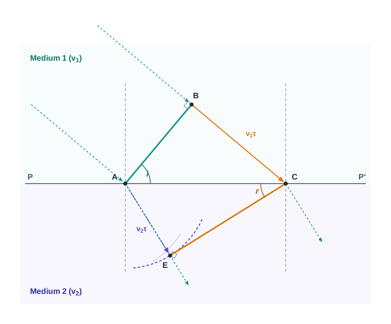
Fig. 10.4 – Refraction of a plane wave entering a denser medium.
Suppose a plane wavefront \(AB\) is travelling in the direction \(A'A\) and strikes the interface at an angle of incidence \(i\), as in Fig. 10.4. The wavefront does not reach the whole surface at once — one end reaches first, and the other end has some distance still to go. Let \(\tau\) be the time taken by the wavefront to cover the remaining distance \(BC\) in medium 1. Since distance = speed × time,
\[BC = v_1 \tau\]
During this same time \(\tau\), the part of the wavefront that has already entered medium 2 (starting from point \(A\)) has been travelling at the new speed \(v_2\). To find where its wavelet has reached, we draw a sphere of radius \(v_2\tau\) centred on point \(A\) in the second medium. From point \(C\) we then draw a tangent plane \(CE\) to this sphere. Then \(AE = v_2\tau\), and this tangent \(CE\) is exactly the new, refracted wavefront — obtained, as always, as the common tangent to the secondary wavelets.
Now we simply read off the geometry. Consider the two right-angled triangles \(ABC\) and \(AEC\), which share the common side \(AC\). From triangle \(ABC\),
\[\sin i = \frac{BC}{AC} = \frac{v_1 \tau}{AC} \qquad (10.1)\]
and from triangle \(AEC\),
\[\sin r = \frac{AE}{AC} = \frac{v_2 \tau}{AC} \qquad (10.2)\]
where \(i\) and \(r\) are the angles of incidence and refraction respectively. Dividing Eq. (10.1) by Eq. (10.2), the common factors \(\tau\) and \(AC\) cancel, leaving a clean result:
\[\frac{\sin i}{\sin r} = \frac{v_1}{v_2} \qquad (10.3)\]
This one equation carries a powerful physical message. If the ray bends towards the normal (so that \(r < i\), and therefore \(\sin r < \sin i\)), then Eq. (10.3) forces \(v_2 < v_1\) — the speed of light in the second medium must be less than in the first. This is precisely the wave-model prediction we highlighted in the introduction, and it is the exact opposite of the corpuscular model’s prediction. Later experiments (Foucault’s measurement in water) confirmed that the wave theory is the correct one.
To recover the familiar form, we bring in the refractive index. If \(c\) is the speed of light in vacuum, then for the two media we define
\[n_1 = \frac{c}{v_1} \qquad (10.4)\]
\[n_2 = \frac{c}{v_2} \qquad (10.5)\]
These numbers \(n_1\) and \(n_2\) are the refractive indices of medium 1 and medium 2. Being ratios of two speeds, they have no units (they are pure numbers). A larger \(n\) means a slower speed of light in that medium, which is why a denser medium like glass has a higher refractive index.
Substituting \(v_1 = c/n_1\) and \(v_2 = c/n_2\) into Eq. (10.3), and cancelling \(c\), gives the standard form:
\[n_1 \sin i = n_2 \sin r \qquad (10.6)\]
This is Snell’s law of refraction — now derived purely from the wave theory of light.
The wave picture also tells us something the ray picture cannot — what happens to the wavelength. Let \(\lambda_1\) and \(\lambda_2\) be the wavelengths of the light in medium 1 and medium 2. Suppose the distance \(BC\) is exactly one wavelength \(\lambda_1\). Then, in the same time \(\tau\), the distance \(AE\) must be exactly one wavelength \(\lambda_2\) in the second medium. This is because if the crest that was at \(B\) has just reached \(C\) in time \(\tau\), then the crest that started at \(A\) must likewise have reached \(E\) in that same time. Therefore
\[\frac{\lambda_1}{\lambda_2} = \frac{BC}{AE} = \frac{v_1}{v_2}\]
which rearranges to
\[\frac{v_1}{\lambda_1} = \frac{v_2}{\lambda_2} \qquad (10.7)\]
Notice that \(v/\lambda\) is simply the frequency of the wave. Equation (10.7) is therefore telling us that the frequency has the same value on both sides of the boundary. In other words, when a wave passes into a denser medium (where \(v_1 > v_2\)), both its speed of propagation and its wavelength decrease, but its frequency \(\nu\) (equal to \(v/\lambda\)) stays the same.
This frequency-stays-constant rule is a favourite exam trap. Students often assume that “wavelength changes, so colour changes” — but the correct chain is: frequency is unchanged → colour is unchanged; only speed and wavelength change. Also be careful with the two forms of Snell’s law: \(\dfrac{\sin i}{\sin r} = \dfrac{v_1}{v_2} = \dfrac{n_2}{n_1}\), so the ratio of speeds and the ratio of refractive indices are inverted relative to each other.
10.3.2 Refraction at a rarer medium
So far we looked at light entering a denser medium, where it slows down and bends towards the normal. Now let us turn the situation around and consider light passing into a rarer medium — a medium in which light travels faster. In symbols, this is the case \(v_2 > v_1\): the speed in the second medium is greater than in the first.
The Huygens construction proceeds in exactly the same way as before, and the refracted wavefront comes out as shown in Fig. 10.5. The only difference is in the outcome: because the light now speeds up, the ray bends away from the normal, so the angle of refraction is now greater than the angle of incidence. Even so, Snell’s law still holds unchanged: \(n_1 \sin i = n_2 \sin r\).
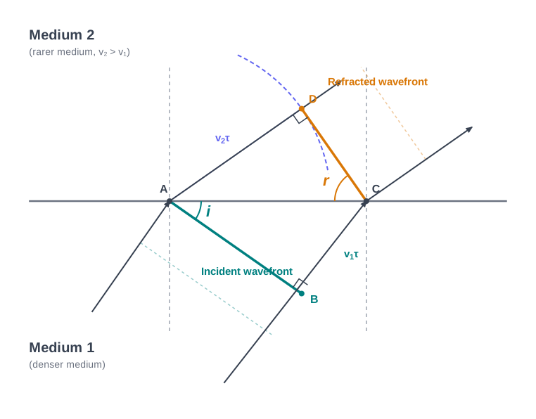
Fig. 10.5 – Refraction of a plane wave entering a rarer medium.
This bending-away has a striking consequence. As we increase the angle of incidence \(i\), the angle of refraction \(r\) grows even faster, and at some special angle of incidence \(r\) reaches its largest possible value of \(90^\circ\) — meaning the refracted ray just grazes along the surface. We call this special incidence angle the critical angle, written \(i_c\), and it is defined by
\[\sin i_c = \frac{n_2}{n_1} \qquad (10.8)\]
Here \(n_1\) is the refractive index of the denser medium the light starts in, and \(n_2\) that of the rarer medium. Since \(r = 90^\circ\) gives \(\sin r = 1\), putting \(i = i_c\) into Snell’s law leads directly to Eq. (10.8).
For any angle of incidence greater than the critical angle, there simply cannot be a refracted wave at all. Instead, the entire light wave is reflected back into the denser medium — a phenomenon known as total internal reflection. You met this effect earlier, from the ray-optics viewpoint, in Section 9.4; here we see that the wave picture arrives at exactly the same condition.
For exams, remember two things about critical-angle problems. First, the light must start in the denser medium (the one with the larger \(n\)) for total internal reflection to be possible. Second, when the rarer medium is air, \(n_2 = 1\), so Eq. (10.8) simplifies to \(\sin i_c = 1/n_1\).
10.3.3 Reflection of a plane wave by a plane surface
Having handled refraction, we now use the very same Huygens construction to derive the law of reflection — the rule that the angle of incidence equals the angle of reflection.
Consider a plane wave \(AB\) falling at an angle of incidence \(i\) on a flat reflecting surface \(MN\), as in Fig. 10.6. Let \(v\) be the speed of the wave in the medium (in \(\text{m s}^{-1}\)) and let \(\tau\) be the time taken by the wavefront to advance from point \(B\) to point \(C\) along the surface. Then
\[BC = v\tau\]
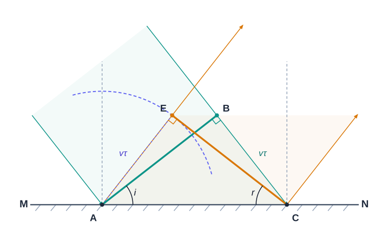
Fig. 10.6 – Reflection of a plane wave by a plane surface.
While that part of the wave is still travelling towards \(C\), the part that struck at \(A\) has already begun to reflect. In the same time \(\tau\), its secondary wavelet spreads out into a sphere of radius \(v\tau\) centred on \(A\). We draw the tangent plane \(CE\) from point \(C\) to this sphere; \(CE\) is the reflected wavefront. Since both wavelets travel in the same medium at the same speed for the same time, their distances are equal:
\[AE = BC = v\tau\]
Now compare the two right-angled triangles \(EAC\) and \(BAC\). They share the side \(AC\), they each contain a right angle, and they have equal sides \(AE = BC\). The two triangles are therefore congruent. Because congruent triangles have equal corresponding angles, the angle of incidence \(i\) equals the angle of reflection \(r\) (both shown in Fig. 10.6). This is the law of reflection.
Once we possess the laws of reflection and refraction, we can understand the working of prisms, lenses and mirrors purely in terms of how wavefronts get reshaped. These devices were already studied in Chapter 9 using rays; here we simply add the wavefront view. The key fact used everywhere is that light travels slower in glass than in air, so whichever part of a wavefront passes through more glass gets delayed more.
In Fig. 10.7(a) a plane wave passes through a thin prism. The lower portion of the wavefront passes through the greatest thickness of glass and is delayed the most, so the emerging wavefront comes out tilted — which is exactly why a prism deviates light.
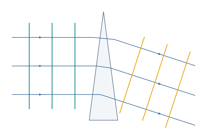
Fig. 10.7(a) – Plane wave refracted by a prism.
In Fig. 10.7(b) a plane wave meets a thin convex lens. Now it is the central part of the wavefront that passes through the thickest glass and is delayed the most. The emerging wavefront therefore develops a hollow at its centre — it becomes spherical and closes in on a single point \(F\), the focus of the lens.
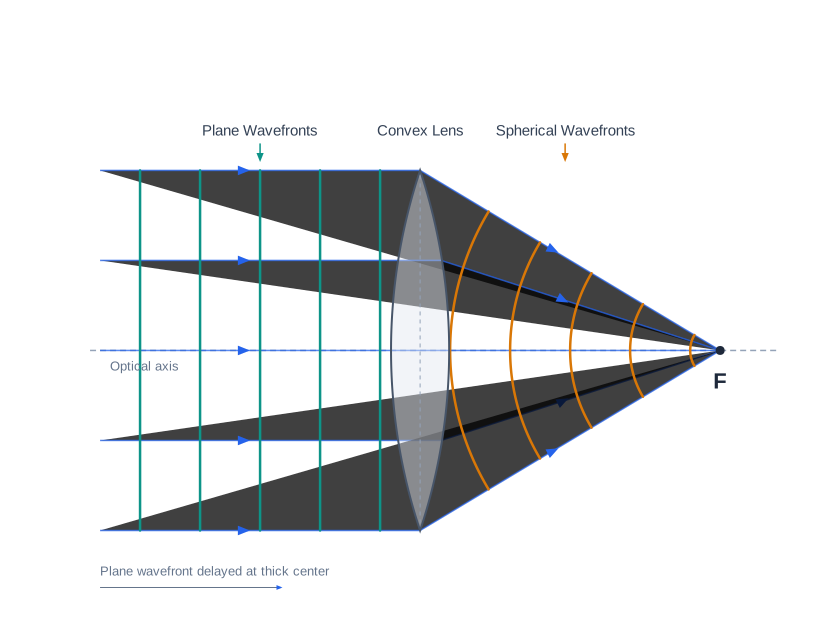
Fig. 10.7(b) – Plane wave refracted by a convex lens.
In Fig. 10.7(c) a plane wave falls on a concave mirror; on reflection the wavefront becomes a spherical wave that converges to the focal point \(F\). In the same way, one can understand how concave lenses and convex mirrors reshape wavefronts.
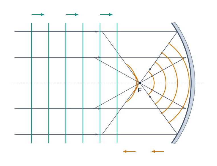
Fig. 10.7(c) – Plane wave reflected by a concave mirror.
This wavefront picture reveals a deep and elegant fact: the total time taken to travel from any point on the object to the corresponding point on the image is the same along every ray. Take a convex lens forming a real image. A ray through the centre of the lens travels a shorter distance, but it also passes through the thickest part of the glass where it moves slowest. A ray near the edge travels a longer distance but through thinner glass, where it moves faster. These two effects balance perfectly, so all rays take equal time and arrive at the image point together, in step.
Before moving on, a note on vocabulary that we will use repeatedly from here: monochromatic light means light of a single frequency (that is, a single pure colour), as opposed to white light, which is a mixture of many frequencies. With that in hand, consider the following worked example, which ties together several ideas about frequency, energy and intensity.
10.4 Coherent and Incoherent Addition of Waves
We now come to the heart of wave optics: what happens when two waves meet at the same point. The pattern they produce together is called an interference pattern, and understanding it lets us finally answer how light added to light can sometimes give darkness.
Everything about interference rests on one rule you already met in Chapter 14 of Class XI — the principle of superposition. It says that when several waves pass through the same point, the total displacement of the medium at that point is simply the sum (more precisely, the vector sum) of the displacements each wave would produce on its own.
To picture this, imagine two needles \(S_1\) and \(S_2\) dipping up and down together in a tray of water, in perfect step, as in Fig. 10.8(a). Each needle sends out a train of circular water waves. At any chosen point, the phase difference between the two arriving waves — how far “out of step” they are — stays fixed and does not drift with time. When two sources behave like this, we call them coherent sources.
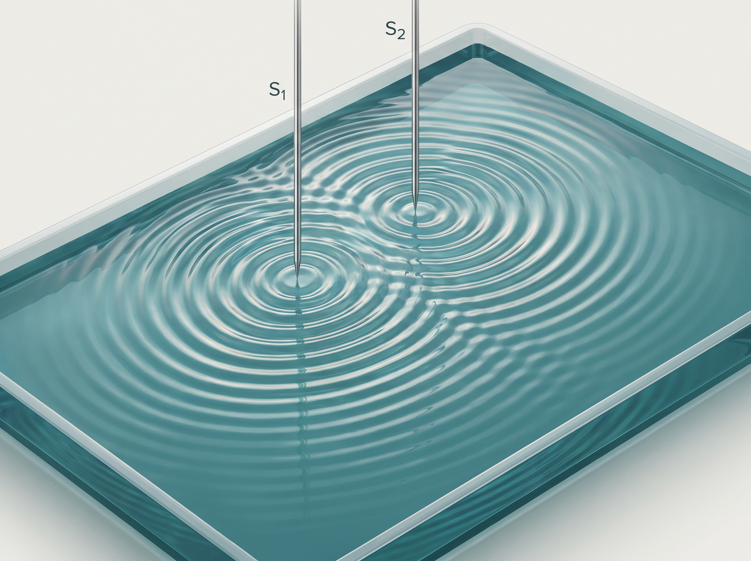
Fig. 10.8(a) – Two needles generating overlapping water waves.
Figure 10.8(b) captures an instant of the overlapping pattern, marking crests (solid circles) and troughs (dashed circles). Where crest meets crest or trough meets trough, the water heaves the most — these are the antinodal lines (marked A, maximum displacement). Where crest meets trough, the water barely moves — these are the nodal lines (marked N, no displacement).
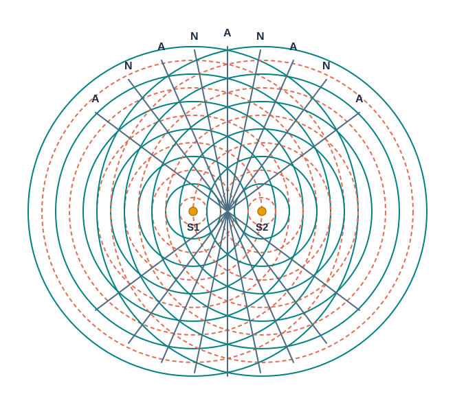
Fig. 10.8(b) – Antinodal and nodal lines in an interference pattern.
A point of equal distance. Let us first take a point \(P\) that is equally far from both needles, so that \[S_1P = S_2P\] Since the two paths are equal, the waves take the same time to reach \(P\). Two waves that leave in phase and travel equal paths therefore arrive in phase.
If the displacement at \(P\) due to source \(S_1\) is \[y_1 = a\cos\omega t\] then the displacement due to \(S_2\) is identical, \[y_2 = a\cos\omega t\] where \(a\) is the amplitude of each wave and \(\omega\) (equal to \(2\pi\nu\)) is the angular frequency, in radians per second. By superposition, the resultant displacement is \[y = y_1 + y_2 = 2a\cos\omega t\]
The resultant amplitude is \(2a\) — double that of a single wave. Since intensity is proportional to the square of the amplitude, and if \(I_0\) is the intensity from one source alone (so that \(I_0 \propto a^2\)), the resultant intensity is \[I = 4I_0\]
In fact every point on the perpendicular bisector of \(S_1S_2\) has zero path difference and so has intensity \(4I_0\). Here the two waves reinforce each other; we call this constructive interference.
A point two full wavelengths apart. Next take a point \(Q\) (Fig. 10.9(a)) where the paths differ by two whole wavelengths: \[S_2Q - S_1Q = 2\lambda\] The wave from \(S_1\) arrives exactly two cycles ahead of the wave from \(S_2\), but two whole cycles means they are back in step. To see this in the equations, recall that one wavelength of path difference corresponds to a full \(2\pi\) of phase; so a path difference of \(2\lambda\) means a phase difference of \(4\pi\). Then \[y_1 = a\cos\omega t, \qquad y_2 = a\cos(\omega t - 4\pi) = a\cos\omega t\] The two are once again in phase, giving intensity \(4I_0\) — constructive interference again.
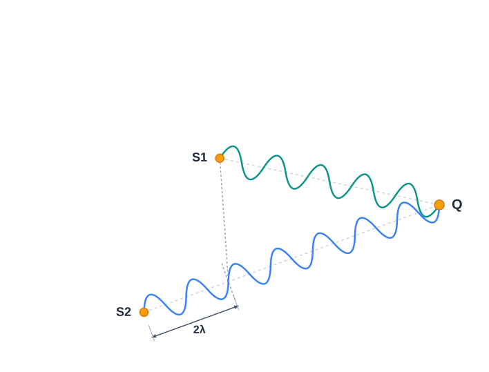
Fig. 10.9(a) – Constructive interference at path difference 2λ.
(In this analysis we assume \(S_1Q\) and \(S_2Q\) are both much larger than the separation \(d\) between the sources. Then, even though the two paths are not equal, the two amplitudes reaching \(Q\) are very nearly the same.)
A point two-and-a-half wavelengths apart. Now take a point \(R\) (Fig. 10.9(b)) where \[S_2R - S_1R = -2.5\lambda\] The wave from \(S_1\) now arrives two-and-a-half cycles behind — that is, exactly half a cycle out of step. A path difference of \(2.5\lambda\) corresponds to a phase difference of \(5\pi\), so \[y_1 = a\cos\omega t, \qquad y_2 = a\cos(\omega t + 5\pi) = -a\cos\omega t\] Here \(y_2\) is the exact negative of \(y_1\): crest of one falls on trough of the other, and they cancel completely, giving zero intensity. This mutual cancellation is destructive interference — and this is precisely how two light waves can add up to darkness.
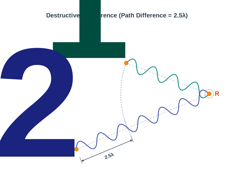
Fig. 10.9(b) – Destructive interference at path difference 2.5λ.
Summarising the two conditions. For two coherent sources \(S_1\) and \(S_2\) vibrating in phase, and any point \(P\), the outcome depends only on the path difference (the symbol \(\sim\) below just means the magnitude of the difference between \(S_1P\) and \(S_2P\)):
\[S_1P \sim S_2P = n\lambda \qquad (n = 0, 1, 2, 3, \dots) \qquad (10.9)\]
gives constructive interference with resultant intensity \(4I_0\). On the other hand,
\[S_1P \sim S_2P = \left(n + \tfrac{1}{2}\right)\lambda \qquad (n = 0, 1, 2, 3, \dots) \qquad (10.10)\]
gives destructive interference with resultant intensity zero.
A general point with any phase difference. Real points on the screen lie between these extremes. Let a general point \(G\) (Fig. 10.10) have a phase difference \(\phi\) between the two waves. Then \[y_1 = a\cos\omega t, \qquad y_2 = a\cos(\omega t + \phi)\] and the resultant is \[y = y_1 + y_2 = a\left[\cos\omega t + \cos(\omega t + \phi)\right]\] Using the trigonometric identity \(\cos A + \cos B = 2\cos\!\left(\dfrac{A+B}{2}\right)\cos\!\left(\dfrac{A-B}{2}\right)\), this becomes \[y = 2a\cos\!\left(\tfrac{\phi}{2}\right)\cos\!\left(\omega t + \tfrac{\phi}{2}\right)\]
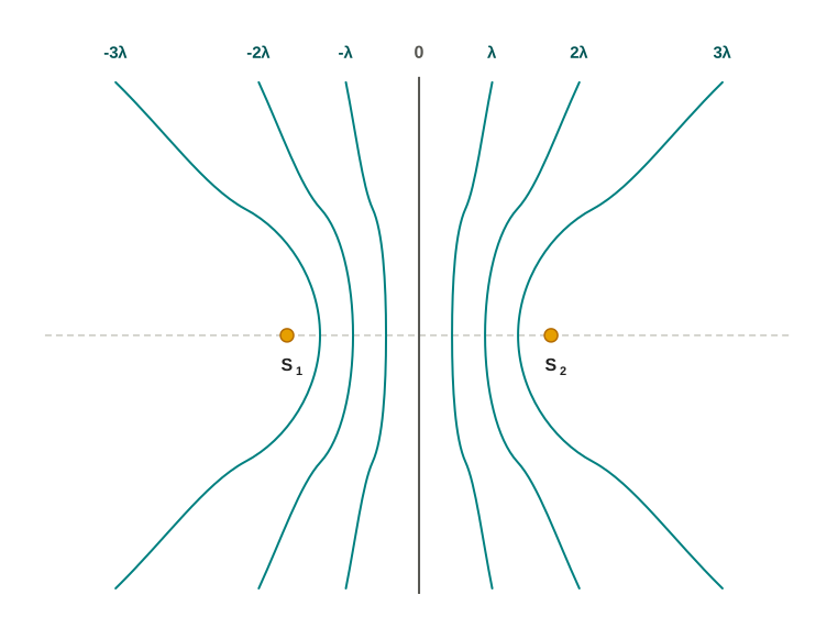
Fig. 10.10 – Locus of maxima for two coherent sources.
The resultant amplitude is \(2a\cos(\phi/2)\), so the intensity at that point is
\[I = 4I_0\cos^2\!\left(\tfrac{\phi}{2}\right) \qquad (10.11)\]
This single formula contains both special cases. When \(\phi = 0, \pm 2\pi, \pm 4\pi, \dots\) (matching Eq. 10.9), \(\cos^2(\phi/2) = 1\) and we get maximum intensity — constructive interference. When \(\phi = \pm\pi, \pm 3\pi, \pm 5\pi, \dots\) (matching Eq. 10.10), \(\cos^2(\phi/2) = 0\) and we get zero intensity — destructive interference.
Coherent versus incoherent — why a stable pattern needs coherence. If the two sources are coherent (the needles dipping steadily), then the phase difference \(\phi\) at each point stays fixed, so the bright and dark regions stay put: we get a stable interference pattern. But if the two sources do not keep a constant phase difference — if \(\phi\) at each point jumps about very rapidly — then the positions of the maxima and minima shift around just as rapidly. Our eyes (and instruments) cannot follow such fast changes and instead record a time-averaged intensity. Since the average value of \(\cos^2(\phi/2)\) over all phases is \(\tfrac{1}{2}\), Eq. (10.11) averages to
\[I = 2I_0 \qquad (10.12)\]
the same everywhere — no fringes at all.
This is exactly what happens when two ordinary, separate light sources shine on a wall: their intensities just add up and no fringes appear.
For exams, three points from this section are tested repeatedly: converting a path difference into a phase difference using “one wavelength \(= 2\pi\)”; remembering that combined intensity is \(4I_0\) (not \(2I_0\)) at a bright fringe because amplitudes add before squaring; and knowing that overall energy is conserved, with the brightness of maxima exactly compensating the darkness of minima.
10.5 Interference of Light Waves and Young’s Experiment
In the previous section we saw how two coherent sources produce a stable pattern of bright and dark regions. We now try to make this happen with light, and we immediately run into a problem.
Suppose we take two separate sodium lamps and use them to light up two pinholes \(S_1\) and \(S_2\), as in Fig. 10.11. Surprisingly, no interference fringes appear on the screen at all. The reason lies in how ordinary light sources emit. A source like a sodium lamp does not send out one smooth, unbroken wave; instead its light suffers sudden, random jumps in phase roughly every \(10^{-10}\) seconds. Two independent lamps therefore have no fixed phase relationship — they are incoherent — and, as we learned in Section 10.4, their intensities simply add up with no fringes.
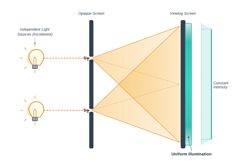
Fig. 10.11 – Two independent sources produce no interference fringes.
Young’s ingenious solution. The British physicist Thomas Young found a clever way to “lock” the phases of the two sources. Instead of using two lamps, he first made a single pinhole \(S\), lit by a bright source. The light spreading out from \(S\) then fell on two closely spaced pinholes \(S_1\) and \(S_2\) cut into an opaque screen, as in Fig. 10.12(a).
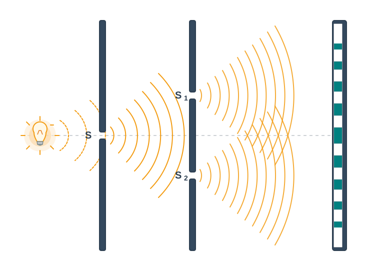
Fig. 10.12(a) – Coherent sources in Young’s experiment.
Because \(S_1\) and \(S_2\) are now both fed by the same original wave from \(S\), any abrupt phase change in \(S\) shows up as an identical phase change in the light leaving both \(S_1\) and \(S_2\). Their phase difference therefore stays fixed — the two are locked in step. In other words, \(S_1\) and \(S_2\) act as genuinely coherent sources, just like the two synchronised needles of our water-wave example in Fig. 10.8(a).
The spherical waves spreading out from \(S_1\) and \(S_2\) overlap and produce interference fringes on the screen \(GG'\), as shown in Fig. 10.12(b). We can now find exactly where the bright and dark bands fall using the path-difference analysis of Section 10.4.
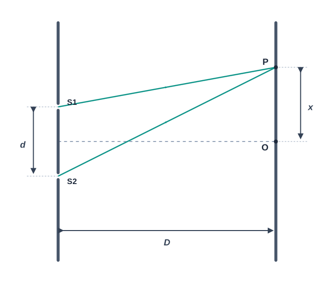
Fig. 10.12(b) – Geometry of the double-slit setup.
Finding the path difference. Let the two slits be separated by a small distance \(d\), and let the screen be a large distance \(D\) away. Consider a point \(P\) on the screen at a height \(x\) above the central point \(O\) (the point directly opposite the midpoint of the slits), as in Fig. 10.12(b). The two path lengths are \[S_1P^2 = D^2 + \left(x - \tfrac{d}{2}\right)^2, \qquad S_2P^2 = D^2 + \left(x + \tfrac{d}{2}\right)^2\] Subtracting one from the other, the \(D^2\) terms cancel and we get \[S_2P^2 - S_1P^2 = 2xd\] The left side factorises as \((S_2P - S_1P)(S_2P + S_1P)\). Since the screen is far away (\(D \gg d\) and \(D \gg x\)), both path lengths are very nearly \(D\), so their sum \(S_2P + S_1P \approx 2D\). Therefore the path difference is \[S_2P - S_1P = \frac{2xd}{2D} = \frac{xd}{D}\] This simple result — path difference \(= xd/D\) — is the key that unlocks the whole pattern.
Bright and dark fringes. Applying the constructive-interference condition of Section 10.4 (path difference \(= n\lambda\)), we get a bright band wherever \(\dfrac{xd}{D} = n\lambda\). That is,
\[x = x_n = \frac{n\lambda D}{d}; \quad n = 0, \pm 1, \pm 2, \dots \qquad (10.13)\]
Applying the destructive-interference condition (path difference \(= (n+\tfrac{1}{2})\lambda\)) gives a dark band wherever \(\dfrac{xd}{D} = \left(n+\tfrac{1}{2}\right)\lambda\). That is,
\[x = x_n = \left(n + \tfrac{1}{2}\right)\frac{\lambda D}{d}; \quad n = 0, \pm 1, \pm 2 \qquad (10.14)\]
Here \(x_n\) is the position of the \(n\)-th fringe measured from the centre (in metres), \(\lambda\) is the wavelength of light, \(D\) the slit-to-screen distance, and \(d\) the slit separation. These alternating bright and dark bands are called fringes, and a computer-generated example is shown in Fig. 10.13 (drawn for \(d = 0.025\ \text{mm}\), \(D = 5\ \text{cm}\) and \(\lambda = 5 \times 10^{-5}\ \text{cm}\)).

Fig. 10.13 – Interference fringes in Young’s experiment.
Fringe width. Equations (10.13) and (10.14) both have equal steps of \(\lambda D/d\) between one fringe and the next, which is why the pattern is equally spaced. The gap between two consecutive bright (or two consecutive dark) fringes is called the fringe width \(\beta\). Subtracting the position of the \(n\)-th bright fringe from the \((n+1)\)-th in Eq. (10.13):
\[\beta = x_{n+1} - x_n = \frac{\lambda D}{d}\]
For exams, the relation \(\beta = \lambda D/d\) is the single most-used result of this section. Remember that fringe width grows with \(\lambda\) and \(D\) but shrinks as the slit separation \(d\) increases, that the central bright fringe sits at \(x = 0\) (the \(n = 0\) case), and that bright and dark fringes always alternate and are equally spaced.
10.6 Diffraction
Look carefully at the edge of the shadow cast by any opaque object. Right at the boundary between light and shadow, you will not find a perfectly sharp edge; instead there are faint alternating dark and bright regions, rather like the fringes of interference. This bending and spreading of light near edges is called diffraction.
Diffraction is not special to light — it is a general property shown by all waves: sound waves, water waves, light waves, even matter waves. The reason we so rarely notice the diffraction of light in daily life is that the wavelength of light is far smaller than the size of most everyday obstacles. When the wavelength is tiny compared with the obstacle, the bending is far too slight to see, and light appears to travel in straight lines.
Diffraction still leaves its mark in subtle ways, though. It sets the ultimate limit on how finely our eyes, telescopes and microscopes can resolve detail. And it produces some everyday beauty too — the shifting rainbow colours you see on the surface of a CD are a diffraction effect. Let us now study diffraction in detail, beginning with the simplest case: a single narrow slit.
10.6.1 The single slit
While discussing Young’s experiment we noted that a single narrow slit acts as a fresh source from which light spreads out. In fact, even before Young, early experimenters — including Newton — had observed that light spilling through narrow holes and slits seems to turn around corners and creep into regions where we would expect a clean shadow. Such effects can only be properly understood using the wave picture.
Indeed, you are never surprised to hear a voice coming from around a corner, because sound diffracts easily. Light does the very same thing; it just bends so little that the effect is hidden in ordinary life.
The single-slit pattern. Suppose we replace Young’s double slit with a single narrow slit, lit by a monochromatic source. On the screen we now see a broad pattern with a bright band at the centre. On either side of this central bright region lie alternating dark and bright bands, each successive bright band fainter than the last, as shown in Fig. 10.14.
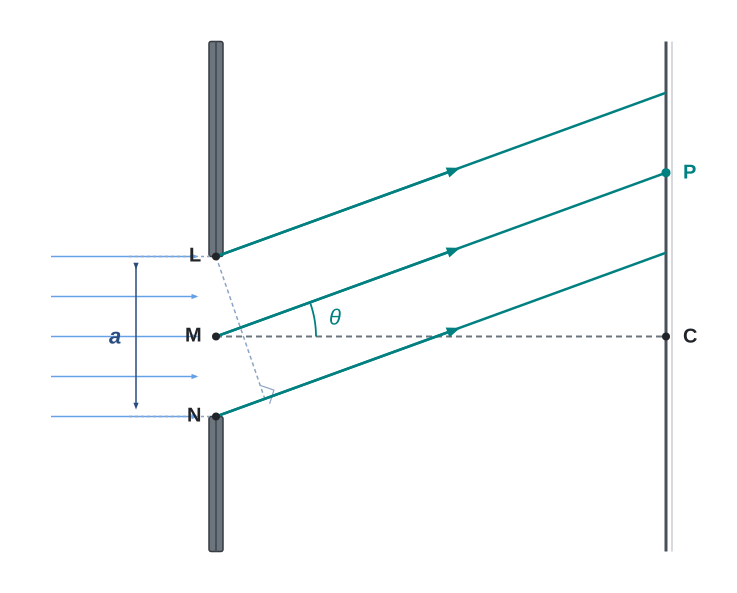
Fig. 10.15 – Geometry of single-slit diffraction.
To understand this, consider Fig. 10.15, which shows a parallel beam of light falling straight (normally) on a single slit \(LN\) of width \(a\). The diffracted light travels on to a screen. Let \(M\) be the midpoint of the slit.
Draw the normal from \(M\); it meets the screen at the central point \(C\). We wish to find the light intensity at some general point \(P\) on the screen. Since the screen is far away, the lines joining \(P\) to the various points \(L\), \(M\), \(N\) of the slit can all be treated as parallel, each making an angle \(\theta\) with the normal \(MC\).
The key idea is to imagine the slit divided into a great many tiny parts, and to add up their contributions at \(P\), each with its correct phase. In other words, we treat every little piece of the wavefront at the slit as a secondary source — Huygens’ idea again. Because the incoming wavefront is parallel to the plane of the slit, all these secondary sources start off in phase with one another.
Now think about what reaches point \(P\) at angle \(\theta\). The wavelet from the top edge \(L\) and the wavelet from the bottom edge \(N\) travel slightly different distances to \(P\); the extra distance across the full slit width is \(a\sin\theta\). This edge-to-edge path difference is what decides whether the contributions build up or cancel.
Consider the direction where the whole slit’s extra path \(a\sin\theta\) equals exactly one wavelength \(\lambda\). Then we can pair the top half of the slit with the bottom half so that each point in the top half is exactly half a wavelength out of step with a matching point in the bottom half. Every such pair cancels, and the total is zero — a dark band (a minimum). The same pairing argument gives a minimum whenever the path difference is a whole number of wavelengths, that is \(a\sin\theta = n\lambda\). For the small angles involved, \(\sin\theta \approx \theta\), so the minima lie at
\[\theta \approx \frac{n\lambda}{a}, \qquad n = \pm 1, \pm 2, \pm 3, \dots\]
Between these minima lie the bright bands. The intensity has its strongest, broadest maximum at the centre, \(\theta = 0\), and weaker secondary maxima at roughly
\[\theta \approx \left(n + \tfrac{1}{2}\right)\frac{\lambda}{a}\]
which grow steadily fainter as \(n\) increases. The full intensity distribution, together with a photograph of the actual pattern, is shown in Fig. 10.14.
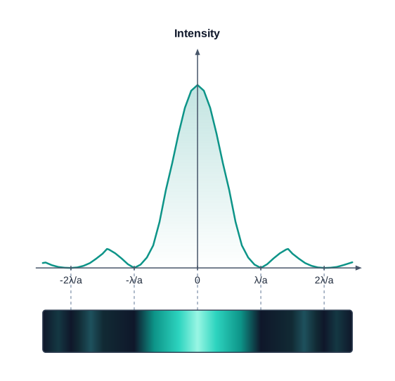
Fig. 10.14 – Intensity distribution in single-slit diffraction.
Here \(\theta\) is the angle measured from the central normal, \(a\) is the slit width (in metres), \(\lambda\) is the wavelength of light, and \(n\) is an integer labelling the band.
Interference versus diffraction. Scientists long debated where “interference” ends and “diffraction” begins. In truth there is no sharp physical line between them — both arise from the superposition of waves. The common convention is simply that when only a few sources combine (as with Young’s two slits) we speak of interference, and when a large number of sources combine (as with the many secondary sources across a single slit) we speak of diffraction.
It is worth noting, then, that the pattern in the actual double-slit experiment is really a superposition of two effects: the single-slit diffraction produced by each individual slit, combined with the two-slit interference between them.
For exams, keep the two “opposite” conditions straight: in a single slit the dark bands satisfy \(a\sin\theta = n\lambda\), whereas in the double-slit interference the bright bands satisfy \(d\sin\theta = n\lambda\). Note too that the central diffraction maximum is about twice as wide as the secondary ones, and that the whole pattern spreads out (\(\theta \propto 1/a\)) as the slit is narrowed.
10.6.2 Seeing the single slit diffraction pattern
One of the delightful things about single-slit diffraction is that you do not need a laboratory to see it — everything you need is probably at home. All it takes is two razor blades and one clear glass electric bulb, preferably one with a straight filament.
The trick is to form a very narrow slit between the parallel edges of the two blades, and then look at the bright filament through that slit. Held steadily right in front of the eye, the slit reveals the diffraction pattern with its bright and dark bands, exactly as described in the previous subsection.
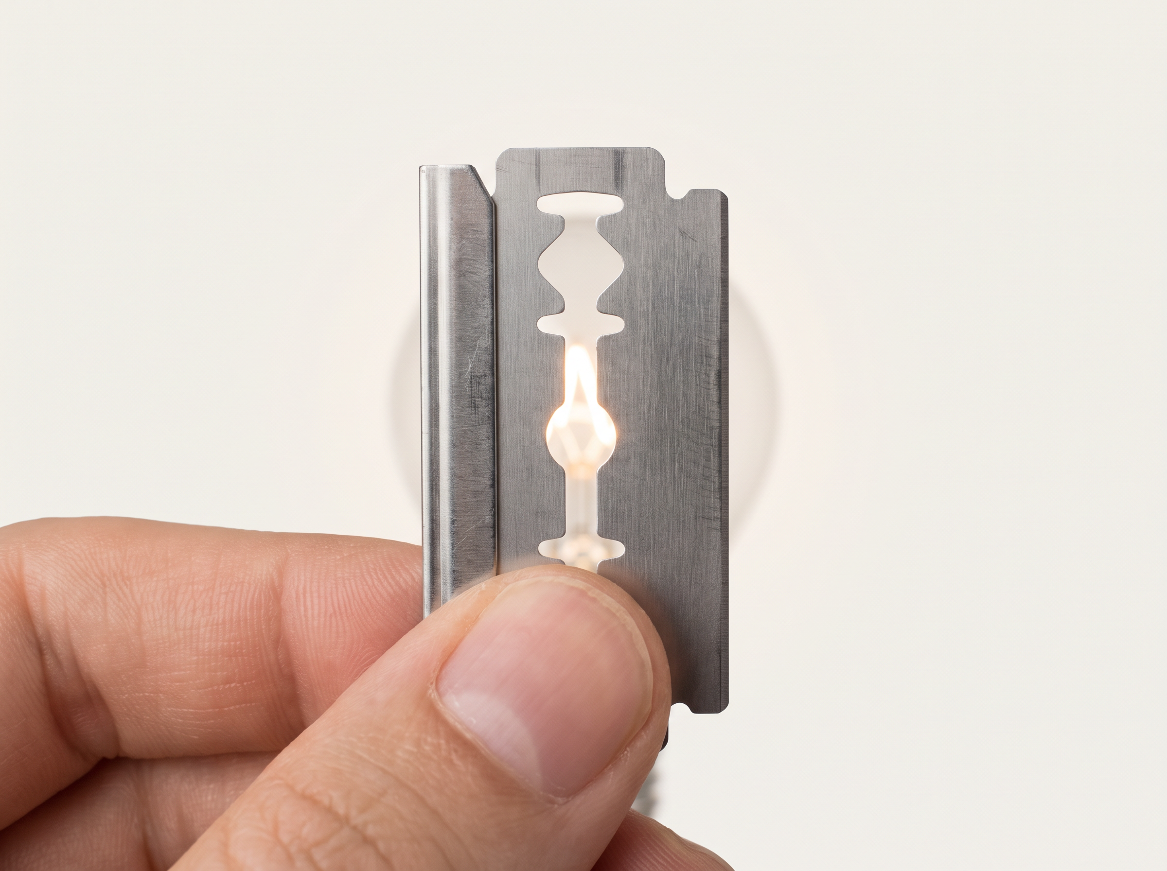
Fig. 10.16 – A makeshift single slit using two razor blades.
In this simple set-up, the glowing filament plays the part of the source slit \(S\) from Fig. 10.14, and the lens of your eye focuses the diffracted light onto its own natural screen — the retina at the back of the eye.
Finally, a point about energy. In both interference and diffraction, light energy is never created or destroyed — it is only redistributed. Wherever the light is reduced to form a dark fringe, it is correspondingly increased somewhere else to form a bright fringe. The books always balance.
For exams, this energy-conservation idea is a favourite conceptual and assertion–reason theme: interference and diffraction do not violate conservation of energy, they merely move energy from the dark regions to the bright ones. Remember also that with white light the central maximum is white while the outer bands are tinged with colour, and that red fringes are wider than blue because red has the longer wavelength.
10.7 Polarisation
We have now explained interference and diffraction, both of which happen for any kind of wave. Polarisation is different: it is a property that belongs to transverse waves alone, and studying it will tell us something new and definite about the nature of light. Let us build the idea up from a simple string.
Hold one end of a long horizontal string whose far end is fixed. If you move your hand up and down steadily, a wave travels along the string in the \(+x\) direction (Fig. 10.17). This wave can be written as
\[y(x,t) = a\sin(kx - \omega t) \qquad (10.15)\]
where \(a\) is the amplitude of the wave, \(\omega\,(= 2\pi\nu)\) is its angular frequency (in radians per second), \(\nu\) is the frequency (in hertz), and \(k\) is the wave number. The wave number is related to the wavelength by
\[\lambda = \frac{2\pi}{k} \qquad (10.16)\]
so \(\lambda\) is the wavelength (in metres). You studied such waves in Chapter 14 of Class XI.
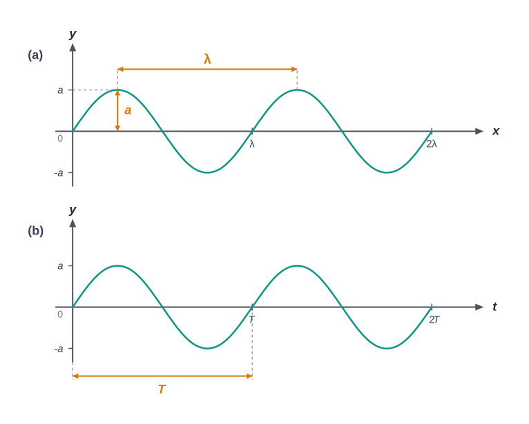
Fig. 10.17 – (a) Spatial and (b) temporal variation of a transverse wave.
Notice a key feature: the displacement here is along the \(y\) direction, while the wave travels along \(x\). The vibration is perpendicular to the direction of travel. A wave like this — where each particle moves at right angles to the direction of propagation — is called a transverse wave.
Because the string vibrates only along \(y\), this particular wave is called a y-polarised wave. Every point on the string moves back and forth along a single straight line, so the wave is also said to be linearly polarised. And since the whole motion stays within the single \(x\)–\(y\) plane, it is likewise called a plane polarised wave — these three names describe the same situation.
We could equally have shaken the string within the \(x\)–\(z\) plane instead, producing a z-polarised wave:
\[z(x,t) = a\sin(kx - \omega t) \qquad (10.17)\]
Both Eq. (10.15) and Eq. (10.17) describe transverse, linearly polarised waves — the displacement is always at right angles to the direction of travel, just confined to a fixed plane.
Now suppose that, instead of keeping to one plane, we keep changing the plane of vibration randomly, very rapidly, from one instant to the next. The displacement is then still always perpendicular to the direction of travel, but its direction within that perpendicular plane keeps jumping about at random. Such a wave is called an unpolarised wave.
Applying this to light. Light waves are transverse: the electric field (the “electric vector”) of a light wave always points at right angles to the wave’s direction of travel. Ordinary light from a source like a sodium lamp is unpolarised — its electric vector points in all possible perpendicular directions, changing at random. We can demonstrate the transverse nature of light very simply using a polaroid.
A polaroid is a thin plastic-like sheet made of long chain molecules all aligned in one direction. When light falls on it, the component of the electric vector along the aligned molecules is absorbed. What passes through is light whose electric vector oscillates in the direction perpendicular to the aligned molecules. This special transmitting direction is called the pass-axis of the polaroid.
So when light from an ordinary source passes through a polaroid sheet \(P_1\), its intensity falls to half, and rotating \(P_1\) has no effect — the transmitted intensity stays constant. This constancy is itself the clue that the incoming light was unpolarised but transverse.
Two polaroids and Malus’ law. Now place a second identical polaroid \(P_2\) before \(P_1\). Light from the lamp is first cut down in intensity on passing through \(P_2\) alone. But now, rotating \(P_1\) produces a dramatic effect on the light coming from \(P_2\) (Fig. 10.18). In one orientation, the intensity passing through \(P_2\) and then \(P_1\) falls to nearly zero; turning \(P_1\) by \(90^\circ\) from that position lets nearly the full beam through.
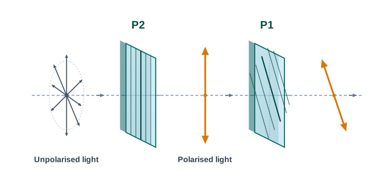
Fig. 10.18 – Polarisation of light by two polaroids.
Here is why. The light emerging from \(P_2\) is polarised along the pass-axis of \(P_2\). Suppose the pass-axis of \(P_2\) makes an angle \(\theta\) with the pass-axis of \(P_1\). Only the component of the electric field along \(P_1\)’s pass-axis, namely \(E\cos\theta\), can get through \(P_1\).
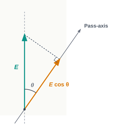
Fig. 10.19 – Resolving the electric vector along the pass-axis.
Since intensity is proportional to the square of the field, the transmitted intensity varies as
\[I = I_0\cos^2\theta \qquad (10.18)\]
where \(I_0\) is the intensity of the polarised light after \(P_1\) and \(\theta\) is the angle between the two pass-axes. This is Malus’ law.
This law explains the whole experiment: a single polaroid cuts the intensity to half, and by adding a second polaroid we can then dial the transmitted intensity smoothly anywhere from that 50% down to zero, just by adjusting the angle between the two pass-axes.
What polarisation tells us, and where it is used. The fact that a polaroid can control the intensity in this way proves that light is a transverse wave — for only transverse waves can be polarised. A longitudinal wave such as sound, whose vibration is along the direction of travel, cannot be polarised at all.
Before we close, here is a worked example that pushes Malus’ law a step further — the surprising case of a polaroid rotated between two crossed polaroids.
10.8 Summary
Huygens’ principle tells us that every point on a wavefront acts as a source of secondary waves (wavelets). These secondary waves add together to build the wavefront at a later instant.
Huygens’ construction shows that the new wavefront is the forward envelope — the common tangent — of all the secondary waves. When the speed of light is the same in every direction, these secondary waves are spherical. The rays are then perpendicular to both the old and the new wavefronts, and the time of travel is the same along every ray. From this construction follow the familiar laws of reflection and refraction.
The principle of superposition applies whenever two or more sources of light reach the same point. In working out the intensity at that point, there is an extra “interference term” over and above the simple sum of the individual intensities. This interference term matters only when it has a non-zero average — and that happens only if the sources have the same frequency and a steady (stable) phase difference, that is, only if they are coherent.
Young’s double slit, with slit separation \(d\), produces equally spaced interference fringes on the screen.
A single slit of width \(a\) produces a diffraction pattern with a broad central maximum. The intensity falls to zero (dark bands) at angles of \(\pm\dfrac{\lambda}{a}, \pm\dfrac{2\lambda}{a}\), and so on, with successively weaker secondary maxima lying in between.
Natural light, such as sunlight, is unpolarised: its electric vector points in all possible directions within the transverse plane, changing rapidly and randomly during any measurement. A polaroid transmits only one component of this vector — the one parallel to its special pass-axis — and the light that comes through is then linearly polarised (also called plane polarised). If this polarised light is viewed through a second polaroid whose axis is rotated through a full turn (\(2\pi\)), the transmitted intensity passes through two maxima and two minima.
10.9 Points to Ponder
A wave from a point source spreads out in every direction, and yet light was long observed to travel along narrow, straight rays. Reconciling these two facts — showing how a single wave theory could account for all the behaviour of light — took the combined insight and experiments of Huygens, Young and Fresnel.
The truly new feature that waves bring is the interference of amplitudes from different sources. Because it is amplitudes (not intensities) that add, the result can be either constructive or destructive — a fact demonstrated directly by Young’s experiment, where light can add to light to give either brightness or darkness.
Diffraction marks the boundary where ray optics breaks down. It is diffraction that ultimately limits how finely a microscope or a telescope can separate two very close objects, and that limit is set by the wavelength of light itself.
Interference and diffraction are not unique to light — most of these effects occur even for longitudinal waves such as sound travelling in air. Polarisation, however, is special: it can occur only for transverse waves like light, and never for longitudinal waves. This is why the very existence of polarisation is proof that light is a transverse wave.
10.10 NCERT Questions
Monochromatic light of wavelength \(589\ \text{nm}\) is incident from air on a water surface. What are the wavelength, frequency and speed of (a) reflected, and (b) refracted light? The refractive index of water is \(1.33\).
What is the shape of the wavefront in each of the following cases: (a) light diverging from a point source; (b) light emerging out of a convex lens when a point source is placed at its focus; (c) the portion of the wavefront of light from a distant star intercepted by the Earth.
- The refractive index of glass is \(1.5\). What is the speed of light in glass? (Speed of light in vacuum is \(3.0 \times 10^8\ \text{m s}^{-1}\).) (b) Is the speed of light in glass independent of the colour of light? If not, which of the two colours — red and violet — travels slower in a glass prism?
In a Young’s double-slit experiment, the slits are separated by \(0.28\ \text{mm}\) and the screen is placed \(1.4\ \text{m}\) away. The distance between the central bright fringe and the fourth bright fringe is measured to be \(1.2\ \text{cm}\). Determine the wavelength of light used in the experiment.
In Young’s double-slit experiment using monochromatic light of wavelength \(\lambda\), the intensity of light at a point on the screen where the path difference is \(\lambda\) is \(K\) units. What is the intensity of light at a point where the path difference is \(\lambda/3\)?
A beam of light consisting of two wavelengths, \(650\ \text{nm}\) and \(520\ \text{nm}\), is used to obtain interference fringes in a Young’s double-slit experiment. (a) Find the distance of the third bright fringe on the screen from the central maximum for the wavelength \(650\ \text{nm}\). (b) What is the least distance from the central maximum where the bright fringes due to both wavelengths coincide?
10.11 Check Your Concepts
Two identical, independent light bulbs of the same colour are placed side by side and shine on a wall. No interference fringes are ever seen. Explain this in terms of coherence, and state the condition two sources must satisfy to produce a stable interference pattern.
According to Huygens’ principle, every point on a wavefront sends out secondary wavelets in all directions. If this is so, a backward-travelling wave (backwave) should also form. Explain how Huygens accounted for the absence of the backwave, and comment on whether his explanation was fully satisfactory.
When light travels from air into glass, state clearly which of the following quantities change and which stay the same: speed, wavelength, frequency, and colour. Give a physical reason for each.
Using the wavefront picture (and the fact that light travels slower in glass than in air), explain why a thin convex lens converts an incoming plane wavefront into a converging spherical wavefront that meets at the focus.
Assertion: We can hear a person speaking from around a corner, but we cannot see that person around the same corner. Reason: Both sound and light are capable of diffraction. — State whether the assertion and reason are individually correct, and whether the reason correctly and completely explains the assertion.
Polarisation can occur for light waves but not for sound waves. Explain why this is so, and state what the phenomenon of polarisation reveals about the nature of light.
In an interference pattern, a bright fringe is brighter than the simple sum of the two individual intensities, while a dark fringe is completely dark. Does this mean that energy is being created at the bright fringes and destroyed at the dark ones? Justify your answer using the principle of conservation of energy.
When unpolarised light passes through a single polaroid, rotating that polaroid does not change the transmitted intensity. But when a second polaroid is added, rotating one of them changes the transmitted intensity dramatically. Explain both observations.
Why does the central bright maximum of a single-slit diffraction pattern become wider when the width of the slit is decreased? Support your answer using the condition for the diffraction minima.
Distinguish between an interference pattern and a diffraction pattern, referring to (a) the number of sources involved and (b) the relative brightness and spacing of the fringes.
In a Young’s double-slit experiment, state (with reasons) what happens to the fringe width if: (i) the entire apparatus is immersed in water; (ii) the screen is moved farther from the slits; (iii) the separation between the two slits is increased.
10.12 Practice with Numericals
Light of wavelength \(600\ \text{nm}\) (in air) enters a transparent medium of refractive index \(1.6\). Taking the speed of light in vacuum as \(3.0 \times 10^8\ \text{m s}^{-1}\), find (a) the speed of the light in the medium, (b) its wavelength in the medium, and (c) its frequency in the medium.
A ray of light travelling inside water reaches the water–air surface. Taking the refractive index of water as \(1.33\) and of air as \(1\), find the critical angle for the water–air interface.
In a Young’s double-slit experiment, the slit separation is \(0.20\ \text{mm}\), the screen is \(1.0\ \text{m}\) away, and light of wavelength \(500\ \text{nm}\) is used. Find (a) the fringe width, and (b) the distance of the fifth dark fringe from the central bright fringe.
Two coherent sources, each producing intensity \(I_0\) at a given point, superpose there with a phase difference of \(120^\circ\). Using \(I = 4I_0\cos^2(\phi/2)\), find the resultant intensity at that point in terms of \(I_0\).
Monochromatic light of wavelength \(500\ \text{nm}\) falls normally on a single slit of width \(0.25\ \text{mm}\). Taking \(\sin\theta \approx \theta\), find the angular positions of the first and second diffraction minima.
Plane-polarised light of intensity \(I_0\) is incident on a polaroid whose pass-axis makes an angle of \(60^\circ\) with the light’s plane of polarisation. (a) Find the transmitted intensity. (b) Find the angle at which the transmitted intensity would instead be \(I_0/2\).
Unpolarised light of intensity \(40\ \text{W m}^{-2}\) passes through two polaroids whose pass-axes are inclined at \(45^\circ\) to each other. Find the intensity of the light emerging after the second polaroid.