Chapter 4: Introduction to Problem Solving
Around the ninth century, a scholar named Abu Abdullah Muhammad ibn Musa al-Khwarizmi worked at the House of Wisdom in Baghdad. He studied the Indian system of writing numbers — the ten digits and the place value system we still use — and wrote a book explaining how to calculate with them.
What made the book remarkable was not the mathematics. It was the style. Al-Khwarizmi did not simply state results. He set out procedures: do this, then do this, then check whether the remainder is zero, and if it is, stop. The steps were so exact that a clerk who understood nothing about why they worked could still follow them and arrive at the correct answer.
Centuries later, European scholars translated his work into Latin. His name, Latinised, became algoritmi, and from it we get the modern word algorithm.
That old idea turned out to be exactly what computers need. A computer has no insight and no common sense. It cannot guess what you meant. It can only follow instructions that are precise, ordered and finite — the very qualities al-Khwarizmi insisted on. So before a single line of a program is written, somebody has to think the solution through and set it out step by step.
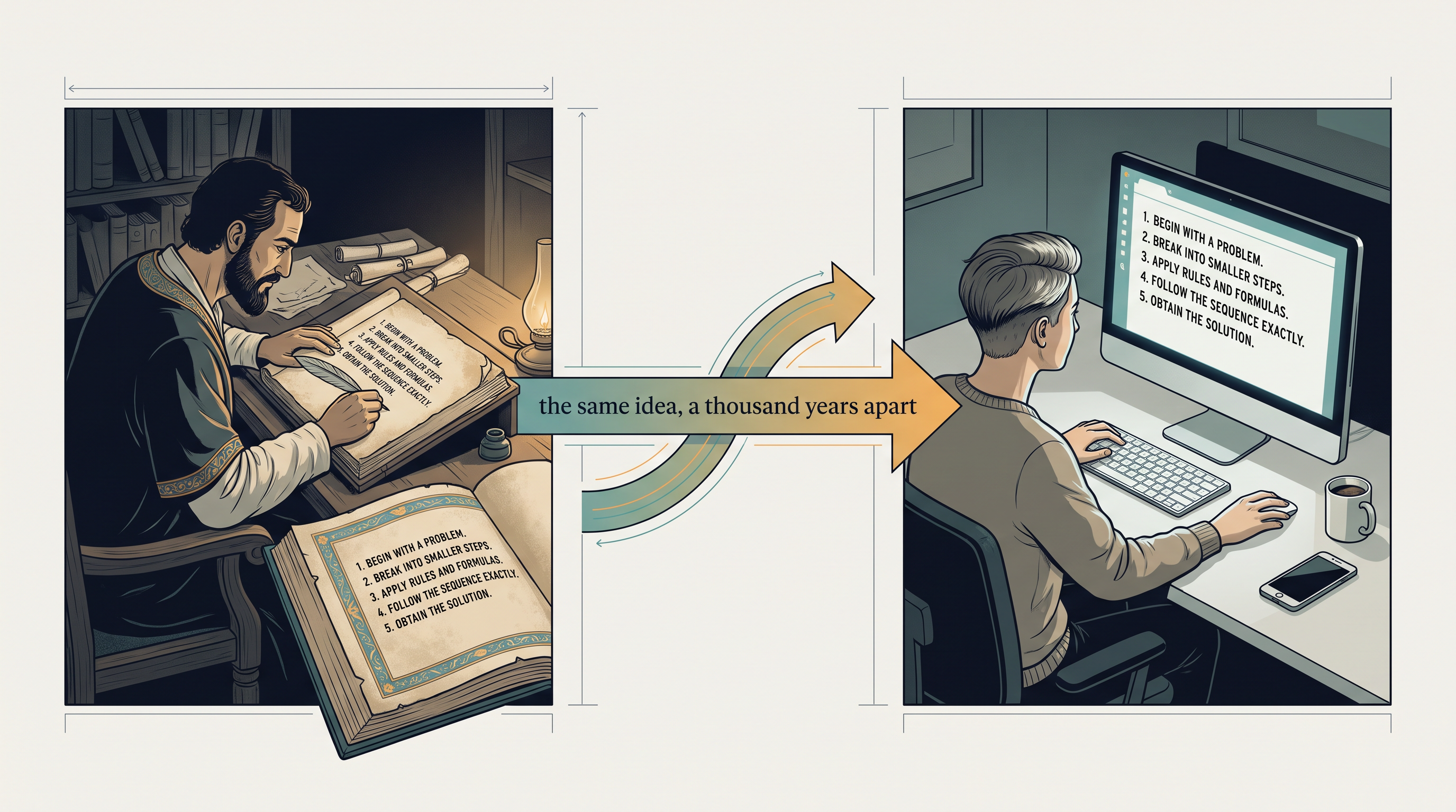
Fig. 4.0 – From a hand-written procedure to a computer program.
Keep these five questions in mind as you read. This chapter answers every one of them.
4.1 Introduction
A school library keeps a register of the books it has issued. When forty books are on loan, a librarian can run a finger down the page and find any entry in a minute. When four thousand books are on loan, and every one of them has to be checked for an overdue date on the same morning, the finger down the page is no longer a method at all. Nothing about the task has become harder to understand. Only its size has changed.
This is where a computer earns its place. It does not think about the library. It counts, compares and copies, at a speed and with a steadiness no person can match, and it does this without getting bored on the three-thousandth record. We use the term computerisation for exactly this move — putting a routine human task in the hands of software so that it is done faster and without slips.
What the computer actually contributes
It is tempting to believe that the computer has solved the library’s problem. It has not. Somebody had to decide what counts as overdue, what the register should store for each loan, what should appear on the list at the end, and in what order. The computer contributed speed and accuracy. Every decision came from a person.
This is worth stating plainly, because it shapes everything else in this chapter. A computer cannot work out what you want. It follows instructions, and it follows them exactly as given, including the ones you gave by mistake. If you ask it to list books issued before today when you meant on or before today, it will happily produce a wrong list very quickly.
From a problem to a working solution
So the real work happens before the machine is involved. Given a task, you must first understand precisely what is being asked, then design a method that would produce the right answer, and only then write that method in a language the computer can act on. That whole journey is what we mean by problem solving.
Notice that the design step sits in the middle, and that it is not optional. A program is a set of instructions written in a programming language for a computer to carry out; it is the last stage, not the first. Writing a program without first designing the method is like laying bricks without a plan — you will produce something, and it may even stand up, but it is unlikely to be the building anyone asked for.
The three stages of this journey are shown in Fig. 4.1. Note how the problem statement narrows into a method, and only then into code.
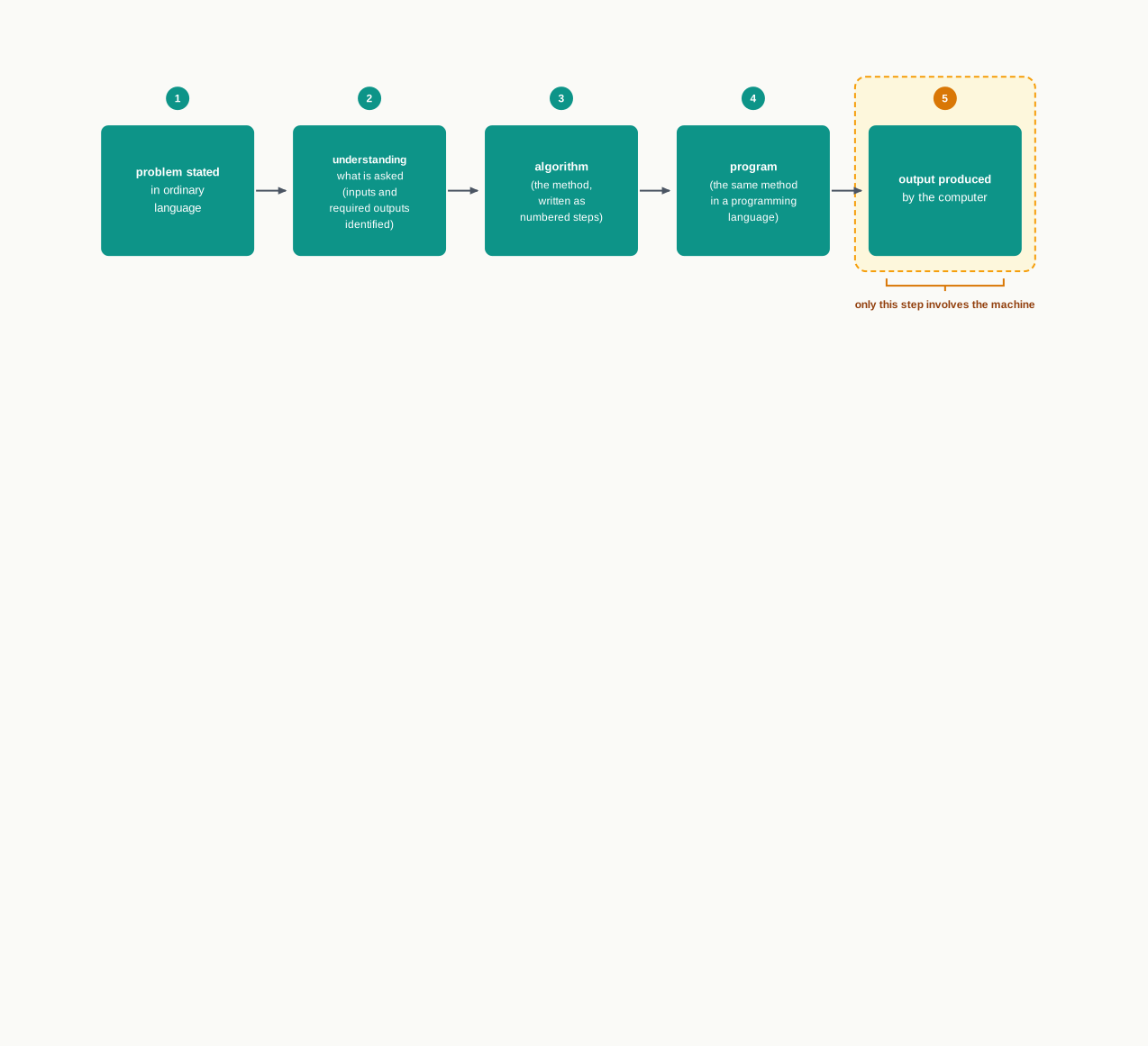
Fig. 4.1 – Stages from problem statement to computer output.
Why the input matters as much as the method
There is a second way a correct method can still give a wrong answer. Suppose the overdue list is perfectly designed, but a book issued on 14 August was entered in the register as 14 September. The program will report it as not yet due, and it will be quite right to do so — given what it was told.
Computer scientists have a blunt name for this: garbage in, garbage out (GIGO).
Where this chapter goes
Everything that follows unpacks the middle stage of Fig. 4.1. We look at the orderly steps a problem is taken through, at what an algorithm is and what makes one good, at the two standard ways of writing an algorithm down, at the three ways control can flow through it, at how to check an algorithm before trusting it, at how to choose between two algorithms that both work, and finally at how a problem too big to think about all at once is broken into parts.
4.2 Steps for Problem Solving
Suppose a fan in your classroom starts making a rattling noise. You do not immediately fetch a screwdriver. You listen to find where the sound is coming from, you decide whether it is the blade, the mounting or the regulator, and only then do you act — or call someone who can. Even a small repair follows a sequence: understand, plan, act, check.
Solving a problem with a computer works the same way, and for the same reason. When a problem is easy, the sequence happens in your head and you barely notice it. When the problem is large, skipping a stage is expensive, because a mistake made early survives every later stage and is discovered last.
Problem solving therefore begins with a precise statement of the problem and ends with a working solution that has been checked. The four stages that take you from one to the other are shown in Fig. 4.2, and each is discussed below.
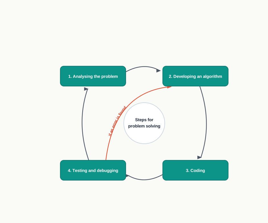
Fig. 4.2 – The four steps of problem-solving.
Notice the arrow that runs backwards, from testing to designing. In practice these stages are not walked through once and left behind. A fault found during testing sends you back to the method, and the loop is travelled again.
To keep the discussion concrete, one small problem will run through all four stages: a class teacher has the marks scored by every student of a class in one subject and wants to know the highest mark, and how many students scored it.
4.2.1 Analysing the Problem
Before anything else, you must be certain what is being asked. This sounds too obvious to state, but it is the stage most often hurried, and a solution built on a misread problem is wrong no matter how elegantly it is written.
Analysing a problem means reading the statement carefully and drawing out three things: what information the solution will be given, what it must produce, and what work has to happen in between. Everything else in the statement is background.
For the teacher’s problem:
- Input — the marks of all the students of the class in one subject.
- Process — find the largest of those marks, then count how many students have exactly that mark.
- Output — the highest mark, and the number of students who scored it.
Writing this down forces the vague parts into the open. Are the marks whole numbers or can they carry a half mark? What should happen if the class list is empty? Is a student who was absent recorded as zero, or not recorded at all? These questions have to be settled now, because each of them changes the method. Settling them later means rewriting work already done.
4.2.2 Developing an Algorithm
Once you know what the solution must do, you work out how it will do it — in ordinary language, not in any programming language. This step-by-step method is the algorithm, and it is the heart of the solution.
For the teacher’s problem the method might run like this: take the first student’s mark as the highest so far; look at each remaining mark in turn, and whenever a mark is larger than the highest so far, treat that one as the new highest; when every mark has been seen, go through the list once more and count how many marks equal the highest.
That is a solution, and you can convince yourself it works without owning a computer. You rarely arrive at it in one attempt, though. A first plan is usually rough — an early version of the above might have found the highest mark and forgotten to count, or might have counted while still updating the highest and produced a wrong count. You refine the plan until it covers everything the problem asks for.
It is also worth knowing that the method above is not the only one. You could sort the marks in descending order and read off the front of the list instead. For a given problem more than one algorithm is usually possible, and part of the work is choosing between them — a question taken up in section 4.7.
4.2.3 Coding
Only now does the computer enter. Coding means converting the finished algorithm into a programming language, following that language’s rules for how statements must be written.
Because the algorithm already fixes what happens and in what order, coding is largely a matter of expressing settled decisions correctly. This is exactly why the earlier stage matters: a programmer who starts typing without a method is trying to design and to express at the same time, and the two kinds of mistake then become impossible to tell apart.
Alongside the code itself, it is normal practice to record how the solution works — what each part does, what assumptions it makes, and why a particular approach was chosen. This record is called documentation. Its value shows up months later, when the program has to be changed by someone who has forgotten the details, or who never knew them. Coding is treated more fully in section 4.8.
4.2.4 Testing and Debugging
A program that has been typed in is not yet a solution. It must be tested — run on chosen inputs and checked against the results you already know to be correct.
Testing asks several things at once. Does the program meet what the user actually needed? Does it respond in a reasonable time? Does it give correct output for every legitimate input, not just the convenient one you tried first? For the teacher’s problem you would test a class where the highest mark is scored once, a class where three students share it, a class where every student has the same mark, and a class list with a single student in it.
Two quite different kinds of fault turn up. A syntax error breaks the rules of the language — a missing bracket, a misspelt keyword — and the program will not run at all, so no output appears. A logical error breaks nothing: the program runs cleanly and produces an answer that is wrong. If our method had compared marks with < where > was meant, it would have reported the lowest mark with complete confidence.
Table 4.1 – Syntax error vs logical error
| Feature | Syntax error | Logical error |
|---|---|---|
| What is wrong | The statement breaks the grammar of the language | The statement is legal but does the wrong thing |
| When it is noticed | Before the program runs | Only when the output is checked |
| Output produced | None — the program does not run | Output appears, and looks perfectly normal |
| How it is found | Reported by the language translator, with a location | By testing with inputs whose correct answer is known |
| Typical cause | A slip while typing | A mistake in the method, or a misread problem statement |
The logical error is the more dangerous of the two, precisely because nothing complains. The only defence against it is deliberate testing.
Correcting the faults found by testing is called debugging, and it is followed by testing again, since a correction can itself introduce a new fault. This continues until no known errors remain.
Large software is tested in stages rather than all at once. The standard stages are unit or component testing, integration testing, system testing, and acceptance testing — first each part on its own, then the parts working together, then the complete system, and finally a check that it does what the user asked for.
Even after delivery the work does not stop. Users report problems that appeared only in real use, ask questions, and request changes. Attending to all of this over the life of the software is called maintenance, and for a program that is used for years it accounts for far more effort than the original writing did.
4.3 Algorithm
Much of what you do in a day is a sequence of steps that you no longer notice. Making a cup of tea, tying a shoelace, filling in a form at a counter, getting ready for school — each is a fixed order of small actions, and doing them out of order does not work. You cannot strain the tea before you brew it.
The same is true of calculations. Suppose you are asked for the greatest common divisor of 24 and 36 — the largest number that divides both of them exactly. One way to find it is to list what divides each number, and then look for the largest number that appears in both lists.
The divisors of 24 are 1, 2, 3, 4, 6, 8, 12 and 24. The divisors of 36 are 1, 2, 3, 4, 6, 9, 12, 18 and 36. The numbers common to both lists are 1, 2, 3, 4, 6 and 12, and the largest of these is 12. So the greatest common divisor of 24 and 36 is 12. Fig. 4.3 shows the two lists side by side.
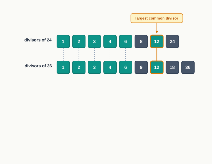
Fig. 4.3 – Finding the greatest common divisor of 24 and 36.
What matters here is not the answer but the shape of the method. It begins somewhere definite, it takes a limited number of steps, each step is something you can actually carry out, and it ends with the answer you wanted. A sequence of steps with those properties is an algorithm.
The method just used can be written out formally.
Notice that nothing in that box mentions Python, or any other language. An algorithm describes a method; it does not commit you to the tools you will use to carry it out.
4.3.1 Why an Algorithm is Needed
A programmer writing code is giving instructions to a machine that will follow them literally. Before those instructions can be written, they have to exist — someone has to know what the first instruction is, and the second, and where the work stops. The algorithm is that plan.
Working without one is possible, and it is a common temptation. What usually happens is that the program is built a statement at a time, each statement patching a problem the previous statement created, until it half works on the one input that was tried. The design was never made; it accumulated.
There is a practical reason to keep the plan separate from the code. A mistake in the plan can be spotted by reading it, and corrected by rewriting a line of English. The same mistake, once buried in a program, has to be hunted down through code that runs perfectly well and simply gives the wrong answer. Catching it early is far cheaper.
Table 4.2 – Algorithm vs program
| Feature | Algorithm | Program |
|---|---|---|
| What it is | The method of solving the problem | The method expressed in a programming language |
| Written in | Ordinary language, or pseudocode, or a flowchart | The exact grammar of a chosen language |
| Read by | People | People, and the computer after translation |
| Can be run directly | No | Yes |
| Depends on the language chosen | No — the same algorithm suits any language | Yes — a change of language means rewriting it |
Because the algorithm is language-independent, a single well-designed method can be turned into a program in Python today and in some other language years later, without the thinking being done again. That is the ordinary case in real software, not the exception.
Almost everything a computer does for you rests on an algorithm underneath: finding a word in a document, sorting a list of names, deciding the route a delivery van should take, matching a query against millions of stored records. In each case the speed is the machine’s contribution and the method is a person’s.
4.3.2 Characteristics of a Good Algorithm
Not every set of instructions deserves the name. “Add a little salt” is an instruction, but it is not a step in an algorithm — two people following it will do different things. A good algorithm has five characteristics.
- Precision — the steps are precisely stated or defined, leaving nothing to the judgement of whoever follows them.
- Uniqueness — the result of each step is uniquely defined, and depends only on the input and on the results of the preceding steps.
- Finiteness — the algorithm always stops after a finite number of steps.
- Input — the algorithm receives some input.
- Output — the algorithm produces some output.
Look back at the divisor method with these in mind. “If d divides a exactly” is precise — there is no room for interpretation. Each step’s result depends only on values already fixed, so two people running it on the same numbers must reach the same answer. The counter d increases every time and the repetition has an upper limit, so the work must end. Two numbers go in and one number comes out.
Finiteness deserves particular care, because it is the one characteristic a careless algorithm loses silently. Precision and uniqueness fail visibly — you notice at once that you cannot follow the step. An endless repetition looks perfectly reasonable on paper.
Alongside these five, there is one habit worth carrying from section 4.2: before writing any algorithm, state clearly what input is to be taken from the user, what processing has to be performed to get the desired result, and what output the user wants. The five characteristics judge an algorithm once it exists; those three questions are how you begin writing one.
4.4 Representation of Algorithms
An algorithm that exists only in your head is of no use to anyone else, and of surprisingly little use to you a week later. Once you have identified the logical steps that lead to a solution, you have to write them down — together with the input they need and the output they produce.
Ordinary sentences work for a short method, but they get clumsy quickly. Two standard ways of setting out an algorithm have come into common use: a flowchart and pseudocode. Either may be used, and both are judged by the same two requirements:
- it should show the logic of the solution and leave out implementation details — nothing about which language will be used, or how a value will be stored;
- it should make plain the order in which the steps are carried out, including where the path splits and where it repeats.
4.4.1 Flowchart — A Visual Representation
A flowchart is a picture of an algorithm. It is drawn using boxes, diamonds and other shapes joined by arrows: each shape stands for one step of the solution, and each arrow shows which step follows which.
The shapes are not decorative. Each one has a fixed meaning, so a reader can tell at a glance whether a step reads data, computes something, or asks a question. The standard symbols are listed in Table 4.3 and drawn in Fig. 4.4.
Table 4.3 – standard flowchart symbols, with the name of each shape and the kind of step it stands for
| Symbol | Function | Description |
|---|---|---|
| Rounded rectangle | Start/End | Also called the terminator symbol. It marks where the flow starts and where it ends. |
| Rectangle | Process | Also called the action symbol. It represents a process, an action, or a single step such as a calculation. |
| Diamond | Decision | A branching point. A yes/no or true/false question is asked, and the path splits into two branches depending on the answer. |
| Parallelogram | Input/Output | Also called the data symbol. It is used to take input or to display output. |
| Arrow | Arrow | A connector that shows the order of flow between the shapes. |
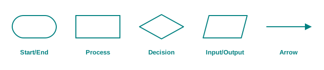
Fig. 4.4 – Standard flowchart symbols.
Consider a small problem: a quiz has a fixed number of marks for each correct answer; given how many answers a student got right, print the total marks scored.
The analysis is short. The input is the number of correct answers and the marks awarded per question. The process is a multiplication. The output is the total.
The same algorithm drawn as a flowchart is shown in Fig. 4.5. Read it downwards: the flow enters at the terminator, passes through a parallelogram where the two values are read, then through a rectangle where the multiplication happens, then through a second parallelogram that displays the result, and leaves at the closing terminator.
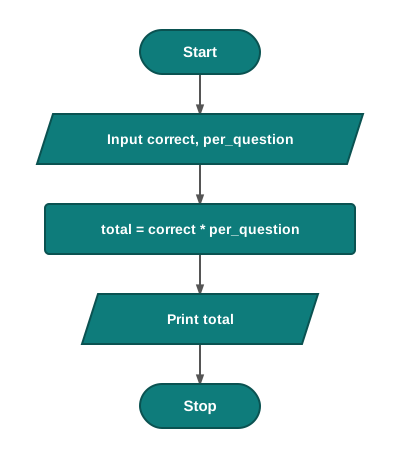
Fig. 4.5 – Flowchart for quiz marks calculation.
4.4.2 Pseudocode
Pseudocode (pronounced soo-doh-kohd) is the other common way of representing an algorithm. The word “pseudo” means “not real”, so pseudocode is literally “not real code”: it looks like a program, but no computer can run it. It is written for a human reader.
There is no official standard for writing pseudocode, and small differences between one book and another are normal. What matters is that each line states one action, unambiguously. A few keywords are used so often that they have become conventional:
INPUTCOMPUTEPRINTINCREMENTDECREMENTIF/ELSEWHILETRUE/FALSE
Take a second problem, from a shop counter: given the price of one item, the number of items bought and the amount the customer hands over, print the bill amount and the balance to be returned.
The same algorithm as a flowchart is shown in Fig. 4.6.
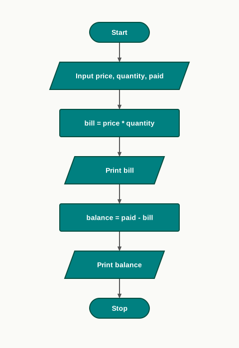
Fig. 4.6 – Flowchart for shop counter bill and balance.
Benefits of pseudocode
Writing the solution first in a human-readable form guards against leaving out an important step. It is easy to forget, while wrestling with the grammar of a language, that the balance must also be printed; it is hard to forget when the whole method is four lines of English in front of you.
Pseudocode is also readable by people who do not program. A shopkeeper cannot check a Python program, but can certainly read COMPUTE balance = paid - bill and confirm that this is what happens at the counter. Getting that confirmation before the program is written is far cheaper than getting it afterwards.
Table 4.4 – flowchart vs pseudocode
| Feature | Flowchart | Pseudocode |
|---|---|---|
| Form | A diagram of shapes joined by arrows | Lines of text in a program-like style |
| Reading the order of steps | Followed by tracing the arrows | Read down the page, line by line |
| Suits | Showing branching and repetition at a glance | Methods with many steps or detailed calculations |
| Effort to change | The diagram usually has to be redrawn | A line is edited or inserted |
| Distance from code | Farther — no statement-like syntax at all | Closer — lines often map one-to-one to statements |
Neither representation is superior. A branching method is usually clearer as a picture; a long sequential method is usually clearer as text. Many programmers sketch a flowchart to settle the shape of the solution and then write pseudocode before coding.
4.5 Flow of Control
Every algorithm you have seen so far has been read straight down the page: first step, second step, third step, stop. That is one possible shape, but it is not the only one. An algorithm may need to choose between two courses of action, or to do the same work several times over.
The order in which the steps of an algorithm are actually carried out is called the flow of control.
Those three possibilities — sequence, selection and repetition — are enough to build any algorithm you will meet in this course, and this section takes them one at a time.
4.5.1 Sequence
In a sequence, every step is executed once, in the order written, and control never turns aside. The quiz-marks method and the shop-counter method of section 4.4 are both sequences: read the values, compute, print, stop.
Sequence is so natural that it is easy to overlook, but two things about it are worth noticing. First, the order carries meaning — a value must be computed before it is printed, as the error box in section 4.4.2 showed. Second, a pure sequence does exactly the same work whatever the input is. Read three values and multiply two of them, and that is what happens for every customer, every time.
Most useful problems are not like that. The library fine depends on whether the book is late; the postage depends on how heavy the parcel is; adding up a week of readings means doing the same small step seven times. For these we need control to leave the straight line.
4.5.2 Selection
Think about the routes between your home and your school. There is usually more than one. In the morning you may take the shortest; in the afternoon, if that road is crowded, you take a longer but quieter one. The choice is not fixed in advance — it is made when you reach the turning, on the basis of what you find there.
That is selection: control checks a condition and, depending on whether the condition is true or false, takes one path or another. Conditions can only ever come out true or false, and such values are called binary values.
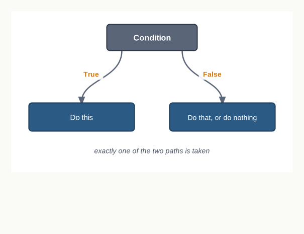
Fig. 4.7 – The branching paths of a selection step.
In pseudocode, the simpler form acts only when the condition holds:
IF <condition> THEN
    steps to be taken when the condition is true
Often, though, something has to happen in the other case as well. The word ELSE introduces it:
IF <condition> THEN
    steps to be taken when the condition is true
ELSE
    steps to be taken when the condition is false
Choosing between two paths
A school library charges a fine of two rupees for each day a book is kept beyond its due date. Books returned on time carry no fine.
The flowchart in Fig. 4.8 makes the split visible. The two branches leave the diamond, do different work, and join again before the result is printed.
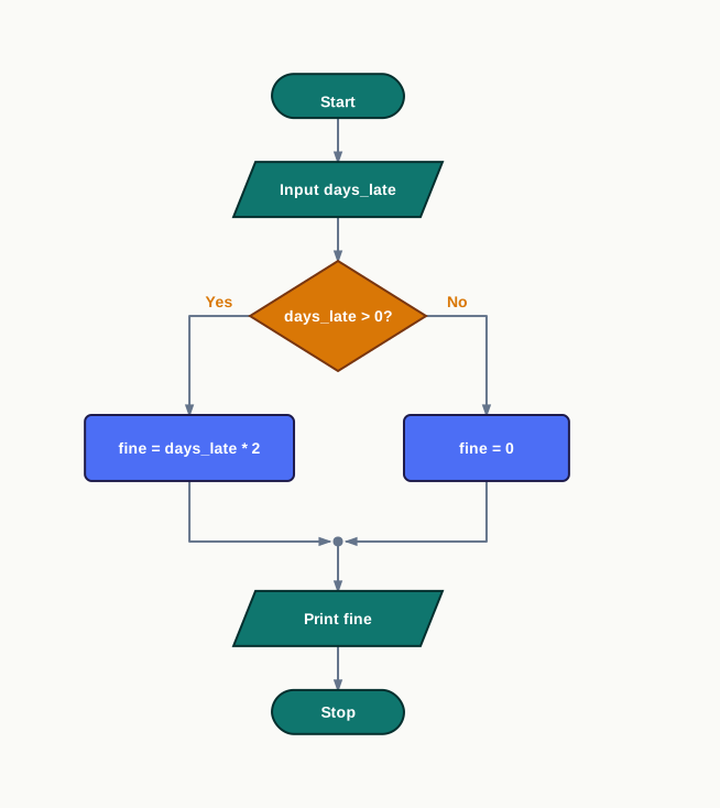
Fig. 4.8 – Flowchart for a library fine with two branches.
Choosing among several paths
Two paths are not always enough. A parcel counter charges by weight: up to 500 grams the charge is 40 rupees; above 500 grams and up to 2000 grams it is 70 rupees; anything heavier costs 120 rupees. Here three outcomes are possible, and they are tested one after another.
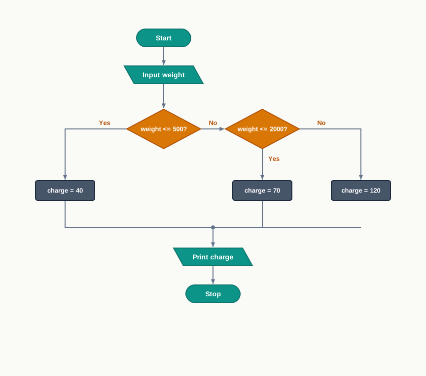
Fig. 4.9 – Flowchart for postal charges with multiple conditions.
4.5.3 Repetition
When you give someone directions you say “walk fifty steps and then turn right”, or “keep walking until you reach the crossing”. Both ask for the same action again and again — one for a stated number of times, the other until something becomes true. Clapping five times, filling a bucket until it overflows, checking each of forty answer scripts: all of these are repetitions.
In an algorithm, repetition — also called iteration, or a loop — means executing a set of steps over and over until a specified condition is satisfied.
Repeating a known number of times
A weather club records the rainfall on each of the seven days of a week and wants the weekly total and the daily average. The same two actions — read a reading, add it to the running total — happen seven times.
The variable day here is a counter: its only job is to keep track of how many times the loop has run. Fig. 4.10 shows the shape this gives the flowchart — an arrow that runs back upward, which is what makes it a loop.
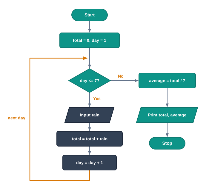
Fig. 4.10 – Flowchart for weekly rainfall showing a loop.
Repeating an unknown number of times
Sometimes you cannot say in advance how many passes are needed. A student is given a book of a certain length and reads a fixed number of pages every day; how many days will the book take? The answer depends on both numbers, and the algorithm must simply keep going until the book is finished.
Here the number of passes is not written anywhere in the algorithm. It emerges from the values supplied, which is exactly why the WHILE construct exists. Tracing it on a small case shows this clearly.
Table 4.5 – repetition with a counter vs repetition with a condition
| Feature | Counter-controlled repetition | Condition-controlled repetition |
|---|---|---|
| Number of passes | Known before the loop begins | Not known until the loop runs |
| What ends it | A counter reaching a fixed limit | A condition about the data becoming false |
| Typical use | Reading a fixed set of readings, marks or items | Working until a target is reached or the data runs out |
| Example in this section | The seven rainfall readings | Days needed to finish a book |
| Main risk | Running one pass too few or too many at the limit | Never stopping, if nothing in the body can make the condition false |
Both kinds are written with WHILE in pseudocode, and the difference lies in what the condition tests — a counter you control, or a value that depends on the input.
4.6 Verifying Algorithms
Think about what a bank’s software is trusted to do. If the module that transfers money credited only half the amount sent, or credited the sender instead of the receiver, the mistake would spread through thousands of accounts before anyone noticed. Software now runs hospital equipment, aircraft systems, examination results and payment counters, and in all of these an error is not an inconvenience but a serious failure. Every part of such a system has to be defined correctly and checked in every way one can think of.
Checking cannot begin at the end. If the method itself is wrong, no amount of careful coding will save it, so the algorithm has to be verified before it becomes a program.
Checking against what you already know
You have done this in mathematics without calling it verification. When you were told that the sum of the first \(N\) natural numbers is \(\frac{N(N+1)}{2}\), where \(N\) is a positive whole number, you could test it on a case small enough to add by hand. Take \(N = 8\): adding \(1 + 2 + 3 + 4 + 5 + 6 + 7 + 8\) gives 36, and the formula gives \(\frac{8 \times 9}{2} = 36\). Try two or three more values and confidence grows.
An algorithm is verified the same way. You choose input values, follow the steps of the algorithm exactly as written — not as you meant to write them — and compare the result with the answer you know to be correct. This is called a dry run.
A dry run helps in two ways: it identifies steps that are incorrect, and it brings to light details or specifics that the algorithm has left out altogether. The second is the one that catches people out, because a missing case does not look like a mistake — it looks like nothing at all.
A method that seems to work
A school wants to know how long a period lasts, given its start time and end time, each in hours and minutes on the same day. The obvious method is to subtract.
INPUT hh1, mm1
INPUT hh2, mm2
COMPUTE hh = hh2 - hh1
COMPUTE mm = mm2 - mm1
PRINT hh, mm
Try it on a period that starts at 9:15 and ends at 10:45. The hours give \(10 - 9 = 1\) and the minutes give \(45 - 15 = 30\), so the answer is 1 hour 30 minutes. That is right, and it is tempting to stop here.
Now take a period from 9:50 to 10:20.
The algorithm is not wrong in an obvious way. It is wrong only when mm2 is smaller than mm1, and the first test happened not to be such a case. This is the whole reason for choosing test inputs deliberately rather than taking the first that comes to mind.
Choosing the test values
A dry run is only as good as the inputs chosen for it. Three kinds are worth including, as suggested in Fig. 4.11: an ordinary value that the algorithm will meet most of the time, a value sitting exactly on a boundary, and a value at the edge of what the problem allows.
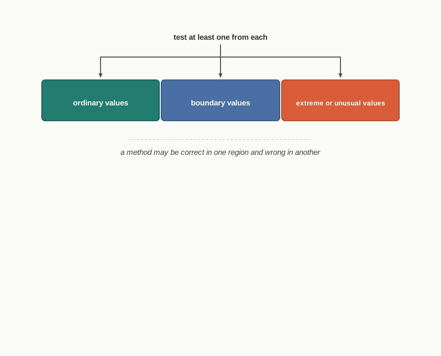
Fig. 4.11 – Choosing test values for a dry run.
For the period-duration problem, a sensible set of tests is shown in Table 4.6.
Table 4.6 – test cases for the period-duration method, with the correct answer and what the first version actually produces
| Start time | End time | Correct answer | First version gives |
|---|---|---|---|
| 9:15 | 10:45 | 1 hour 30 minutes | 1 hour 30 minutes |
| 9:50 | 10:20 | 0 hours 30 minutes | 1 hour −30 minutes |
| 11:30 | 11:30 | 0 hours 0 minutes | 0 hours 0 minutes |
| 8:00 | 14:00 | 6 hours 0 minutes | 6 hours 0 minutes |
Three of the four tests pass. Had only those three been tried, the method would have gone into a program and the fault would have surfaced months later, in a timetable that quietly reported negative minutes.
Correcting the method
The trace tells us what is missing. When the minutes come out negative, one hour of the difference has not yet been converted into minutes. Borrowing 60 minutes from the hours fixes it.
Verifying the corrected method matters as much as verifying the first one — a correction is itself a change that can be wrong.
INPUT held, attended
COMPUTE percent = attended * 100 / held
IF percent > 75 THEN
    PRINT "Allowed"
ELSE
    PRINT "Not allowed"
Dry run it for a student who attended 34 of 40 classes, and for one who attended 15 of 20. Say which case exposes a fault, name the fault, and rewrite the line that fixes it.
4.7 Comparison of Algorithms
A problem rarely has just one method. Section 4.2.2 mentioned two ways of finding the highest mark in a class, and section 4.3 solved the greatest common divisor by listing divisors when other methods exist. Once more than one algorithm solves the same problem, a new question appears: which one should be used?
“Whichever gives the right answer” is not an answer, because they all do. Correctness is the entry requirement, not the deciding factor.
Four ways to test a number for primeness
A prime number is one that has no divisor other than 1 and itself, and testing for primeness matters well beyond arithmetic — it appears in security, in compressing and decompressing files, and in storing and retrieving records. Suppose we want to know whether a given number is prime. There are at least four ways to go about it.
- Starting with the divisor 2, divide the given number and check whether there is any factor. Increase the divisor by one each time and repeat as long as the divisor is less than the given number. If any divisor divides it exactly, the number is not prime.
- As in (i), but instead of testing every number up to the given number, test only up to half of it, because no divisor of a number other than the number itself can be larger than half of it.
- As in (i), but test only up to the square root of the given number.
- Keep a list of prime numbers prepared in advance, and divide the given number only by the primes smaller than it. If none of them divides it exactly, the number is prime.
All four give the correct verdict on every input. The difference lies entirely in how much work each one does.
Counting the work
Take the number 97, which happens to be prime. A prime is the honest case to count, because a composite number stops the search as soon as its first factor turns up, while a prime forces every method to run to the end. Table 4.7 counts the divisions each method performs.
Table 4.7 – number of divisions each method performs while testing 97 for primeness, and the extra storage it needs
| Method | Divisors tested | Number of divisions | Extra memory needed |
|---|---|---|---|
| (i) up to the number | 2 to 96 | 95 | none |
| (ii) up to half the number | 2 to 48 | 47 | none |
| (iii) up to the square root | 2 to 9 | 8 | none |
| (iv) using a stored list of primes | the 24 primes below 97 | 24 | the list of primes must be stored |
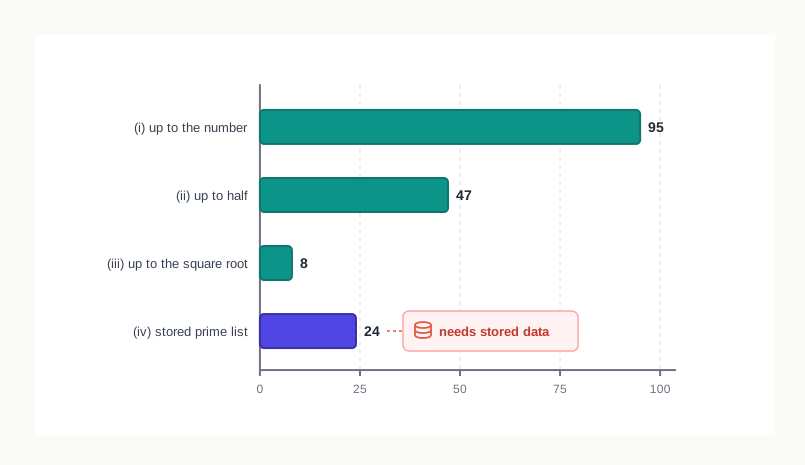
Fig. 4.12 – Work done by four primeness testing methods.
The pattern is easy to read. Method (i) does the most work, because it keeps dividing long after any factor could possibly appear. Method (ii) halves that, and method (iii) reduces it dramatically — from 95 divisions to 8. For a large number the gap widens sharply, and a method that is merely slow on 97 becomes unusable on a number of twelve digits.
Method (iv) is more interesting. It performs fewer divisions than (i) and (ii), because it skips every composite divisor: once 2 has failed, testing 4, 6 and 8 is pointless. But it can do this only because the list of primes is already available, and that list has to be stored somewhere. The saving in work is bought with memory.
Time and space
These two costs have names: time complexity and space complexity.
Comparing algorithms means weighing these two against each other.
Table 4.8 – time complexity vs space complexity
| Feature | Time complexity | Space complexity |
|---|---|---|
| What it measures | The processing time the algorithm needs | The memory the algorithm needs while it runs |
| What increases it | More comparisons, divisions or passes through the data | Storing extra lists, tables or copies of the data |
| Seen in this section | Method (i), which performs 95 divisions for 97 | Method (iv), which must keep a list of primes |
| How it is reduced | Doing less work per input, as method (iii) does | Recomputing values instead of storing them |
| Effect of the other | Saving memory often costs time | Saving time often costs memory |
The last row is the important one. The two costs usually pull in opposite directions: an algorithm that stores results to avoid recalculating them is trading space for time, and one that recalculates to avoid storing is trading the other way. There is no single winner, and the right choice depends on which resource is scarce. On a device with very little memory, method (iii) is the sensible pick even though method (iv) does fewer divisions.
4.8 Coding
Once the algorithm is finalised and verified, it is written out in a programming language chosen by the programmer. This is the third of the four steps of section 4.2, and it is the first point at which the computer becomes involved at all.
The work here is translation, and translation into an unforgiving language. Every programming language lays down rules about how its statements must be formed — which words are reserved, how names may be spelt, where brackets, colons and commas belong, how the end of one statement and the start of the next are marked. These rules are the language’s syntax.
A human listener will understand “school to going I am” without effort. A translator program will not. It compares what you wrote against the rules, and if a single comma is out of place it refuses the whole statement. This strictness feels hostile at first and is in fact protective: a rule that is checked mechanically is a whole class of mistakes that cannot reach the running program.
Why we do not write in the computer’s own language
The processor understands only patterns of 0s and 1s. A program written directly in those patterns — in machine language, also called a low-level language — needs no translation at all and is executed by the hardware exactly as written. In that narrow sense it is the ideal form for a program to take.
It is also close to unwritable. Long strings of binary digits are extremely difficult for people to produce, to read back and to correct, and a single misplaced digit is invisible to the eye. Worse, machine language is tied to the machine. A low-level program runs on one kind of computer only, and moving it to a different type of system means rewriting it.
This difficulty led to the invention of high-level languages, which are much closer to natural language and to ordinary mathematical notation. They are easier to read, to write and to maintain, and they are portable — the same program will run on different types of computer with little or no modification. What they are not is directly understood by the hardware. A wide variety of them exists, among them FORTRAN, C, C++, Java and Python.
Table 4.9 – Machine language vs high-level language
| Feature | Machine language | High-level language |
|---|---|---|
| Form | Binary patterns of 0s and 1s | Words and symbols close to English and to mathematics |
| Understood by the hardware | Directly | Not directly; it must be translated first |
| Ease for the programmer | Very difficult to write, read and correct | Comparatively easy to write, read and maintain |
| Portability | Runs on one kind of computer only; must be rewritten for another | Runs on different types of computer with little or no change |
| Used for | Work that must address the hardware directly | Almost all ordinary program development |
From what you wrote to what runs
A program written in a high-level language is called source code.
Source code cannot be executed as it stands. It has to be translated into machine language, and the translation is done by a compiler or by an interpreter — the two kinds of translator you met in Chapter 1, one translating the whole program before it runs, the other translating and carrying out the statements as it goes. Fig. 4.13 shows where this fits in the journey from algorithm to result.
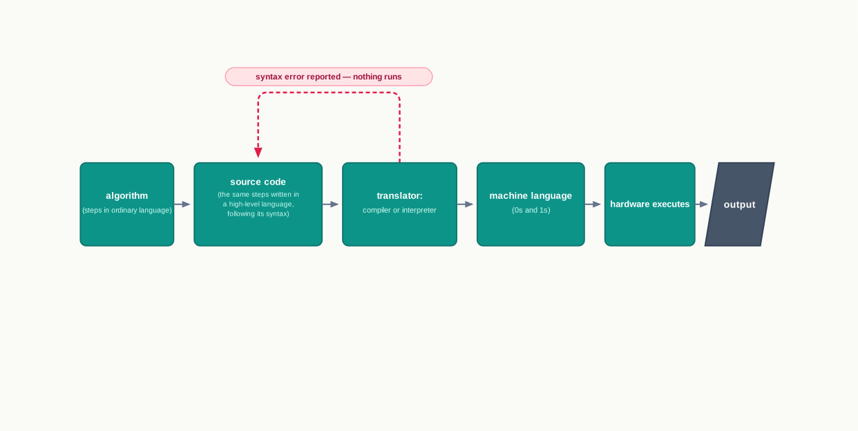
Fig. 4.13 – Translation of source code to machine language.
Notice the branch in the figure. If the source code breaks a rule of the language, the translator stops there and reports it, and no output whatever is produced. That is the syntax error of section 4.2.4, seen from the translator’s side.
Choosing a language, and writing readable code
Several languages could code any of the algorithms in this chapter, and choosing among them means weighing a few practical matters. It depends on the platform — the operating system on which the program will run. It depends on whether what is being built is a desktop application, a mobile application or a web application: desktop and mobile applications are generally developed for a particular operating system and for certain hardware, while web applications are reached from many different devices through a browser and may use resources available over the cloud.
Programs are also written for machines that are not computers in the everyday sense. Digital watches, mp3 players, traffic signals, vehicles, medical equipment and other smart devices all run software, and such embedded systems often call for specialised programming tools, or for programs written in assembly language, closer to the hardware than a high-level language goes.
Whatever the language, one habit belongs to this stage. Record the details of the coding procedure followed and document the solution — comments inside the program explaining what a section does, meaningful names for the quantities held, and a short note of every assumption the method makes. On the day you write it this feels like effort spent on nothing. It repays itself the first time you or anyone else opens the program six months later and has to change one line without breaking the rest.
4.9 Decomposition
Every problem in this chapter so far has been small enough to hold in your head at one time. Real problems often are not.
Consider the software a school would need for its annual sports meet. Six hundred students enter; each may enter more than one event; there are heats and finals; results have to be recorded as they happen, points awarded to houses, a scoreboard kept current, and certificates prepared before the closing ceremony. Sit down to write an algorithm for that, as a single sequence of steps, and you will not get past the first line — not because any part of it is difficult, but because there is no single thread to start pulling.
A problem of this kind is called complex: its solution is not directly derivable. What you do with it is break it up, and the technique of doing so is called decomposition.
Breaking the meet into parts
The sports meet system is not one problem. It is six, each of which is recognisable on its own, as Fig. 4.14 shows.
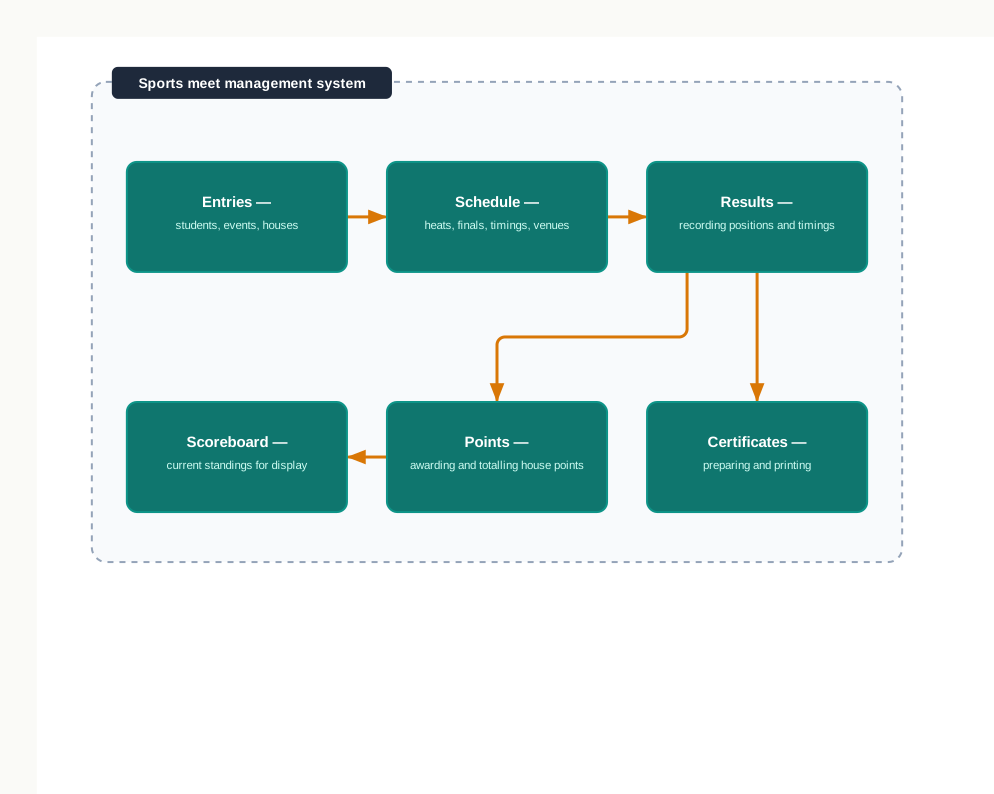
Fig. 4.14 – Decomposition of the sports meet management system.
Each of those boxes is a problem you could actually analyse. Take the fourth. Its input is the recorded positions in an event; its processing awards points by position and adds them to the house totals; its output is the updated totals. That is a problem with a clear input, a clear process and a clear output — precisely the shape section 4.2.1 asked for — and an algorithm for it can be designed, dry run and coded by one person in an afternoon.
Table 4.10 does the same for the rest.
Table 4.10 – the sub-problems of the sports meet system, with the input and output of each
| Sub-problem | Input it receives | Output it produces |
|---|---|---|
| Entries | Student details, chosen events, house | A list of entries per event |
| Schedule | Entries per event, number of tracks or lanes available | Heats and finals, with timings and venues |
| Results | Positions and timings recorded at each event | A stored result for every completed event |
| Points | Positions recorded for an event | Updated house point totals |
| Scoreboard | Current house point totals | The standings, in the form to be displayed |
| Certificates | Results of all events, with names and positions | A printable certificate for each winner |
Notice that the outputs of some boxes are the inputs of others. That is not an accident of this example; it is the usual shape of a decomposed problem, and it is what the arrows in Fig. 4.14 record.
What breaking up buys you
The basic idea is the old one of divide and conquer, and it pays in several ways at once.
- Each sub-problem is small enough to be examined in detail, which the whole problem never was.
- Each sub-problem can be solved independently, and by different people or different teams working at the same time.
- Specific sub-problems can be given to those who are expert at that kind of work — someone who is good at layout takes the certificates, someone comfortable with sorting takes the standings.
- Each part can be tested on its own, so a fault is located within one small piece rather than hunted through the whole system.
- A part that is well designed can often be used again. A module that awards points by position would serve a debate competition or a science quiz with hardly a change.
Decomposition is not confined to software. Problems in mathematics and science are attacked this way, and so are event management in a school, weather forecasting and delivery management systems. Any task large enough to need more than one person is, in effect, being decomposed by whoever assigns the work.
Splitting well, and splitting badly
Decomposition is a design decision, not a mechanical act, and it can be done badly. Two guides help.
Split by the job to be done, not by the order things happen in. “Everything that happens before lunch” is not a sub-problem; “awarding points” is, because it can be stated with an input and an output of its own.
And make the joins as narrow as you can. If two parts need to exchange one list, they are easy to build separately and easy to fit together. If they need to know each other’s inner workings, then splitting them has bought you nothing — you now have two tangled problems instead of one.
When the split is right, something rather satisfying happens: each sub-problem is handled by exactly the method this chapter has set out. You analyse it, design an algorithm, verify the algorithm by a dry run, choose between competing methods if there is a choice, and code it. The four steps of section 4.2 are applied to the parts, and the parts are then assembled into the whole.
4.10 Summary
A computer contributes speed and accuracy, not judgement. It carries out the instructions it is given, exactly as given, so every decision in a solution is made by the person who designs it. Putting a routine human task into software is called computerisation.
Problem solving is the process of understanding a problem clearly, designing a step-by-step method for it, and putting that method into a form the computer can execute. The design comes before the code, always.
Garbage in, garbage out: the correctness of a computer’s output depends on the correctness of the input supplied to it. A well-designed solution therefore checks its input rather than trusting it.
Solving a problem with a computer takes four steps, in order — analysing the problem, developing an algorithm, coding, and testing and debugging. Testing often sends the work back to the design stage, which is normal and not a failure.
Analysing a problem means fixing three things: the input the solution will receive, the processing it must perform, and the output it must produce. A problem that cannot be stated unambiguously has not yet been analysed.
An algorithm is a finite sequence of precisely stated steps which, when followed, solves a given problem or accomplishes a required task. It has a definite beginning, a definite end and a finite number of steps, and it belongs to no particular programming language.
Designing the algorithm first separates two kinds of mistake — a wrong method and a wrong statement — that are impossible to tell apart when code is written straight away. It also allows the method to be checked on paper, discussed with others, and coded in any language afterwards.
A good algorithm has five characteristics: precision, the steps are precisely stated; uniqueness, each step’s result is uniquely defined and depends only on the input and on the results of preceding steps; finiteness, it always stops after a finite number of steps; input, it receives some input; and output, it produces some output.
An algorithm is represented in two common ways, a flowchart and a pseudocode. Both must show the logic of the solution while leaving out implementational details, and both must reveal the flow of control clearly.
A flowchart is a diagram of standard symbols joined by arrows: a rounded rectangle for Start/End, a rectangle for a process, a diamond for a decision, a parallelogram for input or output, and an arrow for the flow between shapes. It shows the shape of a solution at a glance, but grows unwieldy for long or heavily nested methods.
A pseudocode represents an algorithm in a non-formal notation resembling a program. It is written for human reading and cannot be executed by a computer. No fixed standard exists for it; the keywords used by convention are
INPUT,COMPUTE,PRINT,INCREMENT,DECREMENT,IF/ELSE,WHILEandTRUE/FALSE.The order in which the steps of an algorithm are actually carried out is the flow of control, and it takes three forms. In sequence, every step runs once in the order written. In selection, a condition is tested and one branch is chosen while the other is skipped. In repetition, a set of steps is executed again and again until a specified condition is satisfied.
A condition is either true or false, and these two values are called binary values. A conditional with two outcomes is written with
IFandELSE; more than two outcomes are handled by testing conditions one after another, where a later test is reached only when every earlier one has failed. The order of the tests then matters to the result.Repetition, also called iteration or a loop, comes in two kinds. When the number of repetitions is known in advance, a counter tracks how many have been done. When it is not known, the loop tests a condition before each pass and ends when the condition becomes false. Whatever the condition depends on must change inside the loop, or the loop never ends.
An algorithm is verified before it is coded, by a dry run — taking a chosen input, going through the steps by hand, recording the value of every quantity, and comparing the result with the expected result. A dry run identifies incorrect steps and brings to light details the algorithm has left out.
Test values must be chosen deliberately, covering ordinary values, boundary values and extreme or unusual values. A dry run can show that an algorithm is wrong; no number of successful tests can prove it right, and a correction must always be re-checked against the cases that already worked.
A problem usually has more than one correct algorithm. Once correctness is established, algorithms are compared on the processing time they need, called time complexity, and the memory they need, called space complexity. The two often pull against each other: storing results to avoid recalculating them saves time and costs memory, and the reverse is equally true.
After the algorithm is finalised it is coded in a high-level programming language, following that language’s syntax — the rules of spelling, word order and punctuation that govern how statements must be formed.
Machine language, made of 0s and 1s, is understood by the hardware directly but is very difficult for people to write and runs on only one kind of computer. High-level languages are close to natural language, easier to read, write and maintain, and portable across different types of computer, but they are not understood by the hardware directly.
A program written in a high-level language is called source code, and it is translated into machine language by a compiler or an interpreter. If the source code breaks a rule of the language, the translator reports the error and nothing runs at all.
Choosing a language depends on the platform, on whether the application is a desktop, mobile or web application, and on the hardware involved; embedded systems such as digital watches, traffic signals and vehicle controls may need specialised tools or assembly language.
A complex problem is one whose solution is not directly derivable. Decomposition breaks such a problem into smaller sub-problems, each with a clear input and output, which are solved separately — often by different people or teams — and then combined logically to solve the whole.
Decomposition lets each part be examined in detail, assigned to those expert in that kind of work, tested on its own and often reused. The parts must still be tested for correctness and integrated, because faults appear in the joins even when every part is right on its own.
4.11 Key Terms
Algorithm — a finite sequence of precisely stated steps which, when followed, solves a given problem or accomplishes a required task.
Compiler — a translator that converts the whole of a high-level program into machine language before it is run.
Computerisation — the use of a computer, through software, to carry out a routine human task faster and more accurately.
Condition — a test in an algorithm whose outcome is either true or false, and on which a choice or the continuation of a loop depends.
Counter — a quantity kept in an algorithm to record how many times a loop has been repeated.
Debugging — finding the errors in a program, identifying their cause and correcting them, after which the program is tested again.
Decomposition — breaking a complex problem into smaller sub-problems, solving each separately, and combining the solutions logically to solve the whole.
Documentation — the record kept alongside a program of what it does, how it was written and what it assumes, so that it can be understood and changed later.
Dry run — verifying an algorithm by taking a chosen input and going through its steps by hand, recording every value, and comparing the result with the expected result.
Flow of control — the order in which the steps of an algorithm are actually carried out when it runs.
Flowchart — a diagram that represents an algorithm using standard shapes joined by arrows, each shape standing for a step and each arrow showing the order of the steps.
GIGO — garbage in, garbage out — the principle that the correctness of a computer’s output depends on the correctness of the input supplied to it.
High-level language — a programming language close to natural language, easy to read, write and maintain, and portable, but not understood by the hardware directly.
Interpreter — a translator that converts and carries out the statements of a high-level program one at a time as it runs.
Iteration — another name for repetition; one pass through the steps of a loop.
Logical error — a fault in which the statements are legal but the method they express is wrong, so the program runs cleanly and gives an incorrect result.
Loop — a set of steps in an algorithm that is executed repeatedly until a specified condition is satisfied.
Machine language — the low-level language of 0s and 1s that the hardware understands directly, difficult for people to write and tied to one kind of computer.
Maintenance — the work of fixing problems, answering queries and adding features after software has been delivered and is in use.
Portable — able to run on different types of computer with little or no modification.
Problem solving — understanding a problem clearly, designing a step-by-step method that solves it, and putting that method into a form the computer can execute.
Program — a set of instructions written in a programming language for a computer to carry out.
Pseudocode — a representation of an algorithm in a non-formal notation resembling a program, written for human reading and not executable by a computer.
Repetition — a flow of control in which a set of steps is executed again and again while a condition holds.
Selection — a flow of control in which a condition is tested and one branch of the algorithm is carried out while the other is skipped.
Sequence — a flow of control in which every step is executed once, in the order in which the steps are written.
Source code — a program as written by the programmer in a high-level language, before translation into machine language.
Space complexity — a measure of the amount of memory an algorithm needs in order to execute.
Syntax — the set of rules, or grammar, governing how the statements of a programming language must be formed.
Syntax error — a fault in which a statement breaks a rule of the language, so the translator refuses it and the program does not run at all.
Time complexity — a measure of the amount of processing time an algorithm needs in order to run.
4.12 Points to Ponder
A dry run can prove that an algorithm is wrong but never that it is right, since there is always another input you did not try. On what grounds, then, does anyone ever decide that a method is ready to be coded?
Flowcharts and pseudocode both leave out implementational details on purpose. If those details have to be supplied eventually anyway, what exactly is gained by keeping them out at the design stage?
Storing values to avoid recalculating them saves processing time and costs memory; recalculating them saves memory and costs time. Is there any way to tell, before a program is ever run, which of the two a particular problem should trade away?
A method whose steps are precise and unique will give the same result to every person who follows it faithfully. Does that make an algorithm a kind of proof, or is a correct answer on every tested input something weaker than a proof?
Decomposition lets several teams build parts of a system at the same time, yet the faults that are hardest to find turn up in the joins between those parts. Does breaking a problem up genuinely reduce its difficulty, or does it move the difficulty somewhere else?
High-level languages were invented because machine language was too hard for people, and each new generation of languages has moved further from the hardware and closer to how we describe problems in words. Is there a point beyond which a language cannot usefully move, and what would be lost if it did?
4.13 Objective Questions
A step in an algorithm reads “add a suitable amount to the total”. Which characteristic of a good algorithm does this step fail? [1 mark]
- Finiteness
- Precision
- Input
- Output
In a flowchart, a point at which the path splits into two branches is drawn as a [1 mark]
- rectangle
- parallelogram
- diamond
- rounded rectangle
A program prints a total for every student without any error message, but each total is short by one subject. This is an example of [1 mark]
- a syntax error
- a logical error
- a translation error
- no error at all
Which of the following is true of a pseudocode? [1 mark]
- It is executed directly by the computer
- It must follow a standard laid down for all programmers
- It is intended for human reading and cannot be executed directly
- It can be written only after the program has been coded
Fill in the blank: The order in which the steps of an algorithm are actually carried out when it runs is called its ____________. [1 mark]
State whether true or false: A loop in which nothing inside the loop changes the quantity being tested will still stop, because every algorithm must be finite. [1 mark]
Give the full form of GIGO, and state in one line what it warns against. [1 mark]
Assertion (A): A program written in a high-level language cannot be run by the hardware as it stands. Reason (R): The hardware understands only patterns of 0s and 1s. [1 mark]
- Both A and R are true, and R is the correct explanation of A
- Both A and R are true, but R is not the correct explanation of A
- A is true but R is false
- A is false but R is true
Assertion (A): An algorithm should be verified by a dry run before it is coded. Reason (R): A dry run proves that the algorithm will give the correct output for every possible input. [1 mark]
- Both A and R are true, and R is the correct explanation of A
- Both A and R are true, but R is not the correct explanation of A
- A is true but R is false
- A is false but R is true
Match each flowchart symbol in Column I with its function in Column II. [1 mark]
| Column I | Column II |
|---|---|
| a. Rounded rectangle | i. Taking in data or giving out a result |
| b. Parallelogram | ii. A computation or a single step of work |
| c. Rectangle | iii. Showing the order of flow between shapes |
| d. Arrow | iv. Marking where the flow begins and ends |
- Read the fragment and state exactly what it prints. [1 mark]
SET x = 7
IF x > 10 THEN
    PRINT "Large"
ELSE IF x > 5 THEN
    PRINT "Medium"
ELSE
    PRINT "Small"
4.14 Check Your Concepts
Define an algorithm, and state any two characteristics that a good algorithm must have. [2 marks]
Differentiate between a syntax error and a logical error on any two points. [2 marks]
A classmate says that writing the algorithm first is a waste of time, since the program has to be typed anyway. Give three reasons why the algorithm is designed before the code. [3 marks]
Explain what is meant by the time complexity and the space complexity of an algorithm, and give one example of a design choice that reduces one of them at the cost of the other. [3 marks]
Differentiate between a flowchart and a pseudocode on any four points, and state one situation in which each of the two is the better choice. [4 marks]
Name the three ways in which control can flow through an algorithm. Explain each in one line, give a one-line example of each, and state one thing that can go wrong in the third. [4 marks]
A school wishes to have software built for processing its examination results. Explain what is meant by decomposition, list four sub-problems this system could reasonably be broken into with the input and output of each, and give two reasons why the parts must still be tested together after each has been tested on its own. [5 marks]
4.15 Output & Debugging
- Study the fragment below. [2 marks]
SET count = 1, total = 0
WHILE count <= 4, REPEAT the following steps
    COMPUTE total = total + count * count
    INCREMENT count
PRINT total
a. State how many times the steps inside the loop are carried out.
b. State the value printed.- The fragment below is meant to compute the factorial of 5.
SET n = 5, fact = 1
WHILE n > 0, REPEAT the following steps
    COMPUTE fact = fact * n
PRINT fact
State what happens when this fragment is carried out, name the fault, and rewrite the loop correctly. [3 marks]
- A result clerk writes the fragment below to print a remark, where 75 and above earns a distinction and 33 and above is a pass. [3 marks]
INPUT marks
IF marks >= 33 THEN
    PRINT "Pass"
ELSE IF marks >= 75 THEN
    PRINT "Distinction"
ELSE
    PRINT "Fail"
a. State what is printed when the input is 80.
b. Explain why the fragment cannot ever print "Distinction".
c. Rewrite the fragment so that it works as intended.- A depot clerk enters the number of passengers carried on each trip of a route, and enters −1 after the last trip. [3 marks]
SET total = 0, count = 0
INPUT value
WHILE value is not equal to -1, REPEAT the following steps
    COMPUTE total = total + value
    INCREMENT count
    INPUT value
PRINT count, total
The entries made are 12, 8, 20 and then −1. a. Draw a trace table showing value, total and count after every pass of the loop. b. State the two values printed. c. State what the fragment prints if the very first entry is −1.
4.16 Case-Based Questions
- A bus depot charges a monthly pass according to the distance travelled by a student: ₹300 for a distance up to 5 km, ₹500 for a distance above 5 km and up to 10 km, and ₹700 for any distance above 10 km. A clerk enters the distance and the pass amount is to be displayed. [4 marks]
- State the input, the processing and the output for this problem. [1 mark]
- Write the pseudocode for the solution. [2 marks]
- Name one boundary value you would dry run it with, and state why that value is worth testing. [1 mark]
- At a stationery counter, the clerk enters the price and the quantity of one item at a time. Entering a quantity of 0 means there are no more items. The bill is the total of price × quantity for all items, and a discount of 10 per cent is allowed if that total is more than ₹500. [5 marks]
- Name the flow-of-control structures the solution needs, and state what each is needed for. [1 mark]
- Write the pseudocode for the solution. [3 marks]
- Dry run your pseudocode for the entries (₹40, 2), (₹150, 1), (₹60, 5) and then a quantity of 0, and state the amount finally printed. [1 mark]
- A science laboratory wants software to manage the apparatus it issues to classes — recording what exists in the store, issuing items to a class, taking them back, and reporting what is missing at the end of a term. [4 marks]
- Break this problem into four sub-problems, stating the input and the output of each. [2 marks]
- Give two advantages the laboratory gains by having the problem decomposed in this way. [1 mark]
- Describe one kind of fault that would remain hidden while each part is tested on its own, and appear only when the parts are joined. [1 mark]
4.17 Programming Practice
A photocopy shop charges ₹2 per copy for the first 50 copies, ₹1.50 per copy for the next 100 copies, and ₹1 per copy beyond 150 copies, with a fixed handling charge of ₹10 added to every bill. Design the solution that reads the number of copies and prints the amount payable. Submit: the pseudocode, and the three test values you would dry run it with, together with the amount you expect for each. [3 marks]
The marks of a class are entered one after another, and a value of −1 is entered after the last mark. The number of students scoring 75 or more is to be printed, along with the number of students whose marks were entered altogether. Submit: the pseudocode, the matching flowchart, and a dry run on the entries 82, 41, 75, 90, −1 showing every quantity after each pass. [4 marks]
A number is divisible by 3 if the remainder on dividing it by 3 is zero. It is also divisible by 3 if the sum of its digits is divisible by 3. These are two different methods for the same test. Submit: pseudocode for both methods; a count of the steps each performs for the number 987654; a statement of which method has the lower time complexity for large numbers and why; and one honest limitation of the second method. [5 marks]