Chapter 5: Sorting
In 1880 the United States began counting its population, and the counting went badly. Clerks worked through stacks of handwritten returns, copying, grouping and re-grouping them by hand. The results took roughly seven years to compile — so long that the figures were stale before they were published, and the next census was already close.
A young engineer named Herman Hollerith proposed a different approach. Each person’s details would be punched as holes into a card, and machines would read the cards electrically. The important part is what sat beside his tabulating machine: a sorting box. Cards were fed through, and the machine directed each one into the compartment where it belonged. Only after the cards had been brought into order could they be counted meaningfully — all the cards for one state together, all the cards for one age group together.
The 1890 count was completed in a fraction of the earlier time. What made that possible was not faster counting. It was ordering.
The same lesson holds inside a computer today. A list of ten numbers can be arranged in almost any way you like and nobody notices. A list of ten lakh cannot. How you put those elements in order decides whether an answer arrives in a moment or never arrives at all.
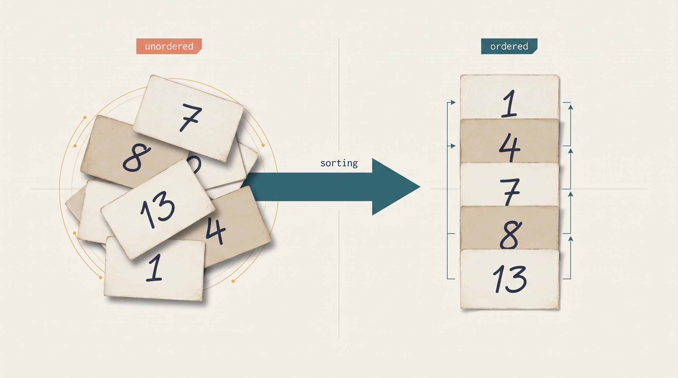
Fig. 5.0 – Sorting transforms unordered data into an ordered arrangement.
Keep these five questions in mind as you read. Each one is answered somewhere in this chapter.
5.1 Introduction
Open any dictionary and you will find the words running from a towards z. Walk into an examination hall and the seats are laid out by roll number. Look at a shop’s rate list and the items are grouped so that a price can be found without reading every line. None of these arrangements happened by accident. Somebody decided the order first, and everything that follows became easier because of it.
A computer works with the same advantage. Data stored in a jumble is still data — every value is there, nothing is lost — but almost every useful question asked about it becomes slower to answer. Putting the values into a chosen order before the questions arrive is one of the oldest and most useful ideas in computing, and it has a name.
5.1.1 What It Means to Sort a Collection
Sorting is the process of arranging the elements of a collection into a definite order decided in advance. The elements themselves do not change; only their positions do. A list holding the numbers 8, 7, 13, 1 and 4 still holds exactly those five numbers after sorting — but now they sit as 1, 4, 7, 8 and 13.
For numbers, two orders are used constantly. In ascending order each element is smaller than or equal to the one after it, so the list runs from the smallest value to the largest. In descending order the arrangement is reversed, and the list runs from the largest value down to the smallest. Nothing in the idea of sorting forces one choice over the other; the problem being solved decides it. A merit list of marks is usually wanted in descending order, while a list of bus departure times is wanted in ascending order.
Strings can be ordered too. A list of names can be arranged alphabetically from a to z, or from z to a, or — if the problem calls for it — by the length of each name. Notice that these are three different orders on the same collection, which tells you something important: sorting is never fully described until you say what “in order” is going to mean.
Sorting Happens Inside the List
In this chapter the collection is a Python list, and the sorting is done inside that same list. Lists are mutable, which means an element can be replaced by assigning to its index — numbers[2] = 40 changes the third element in place, and no new list is created. Every technique you are about to study relies on this. Elements are moved about within the original list by assignment and by exchanging values, and when the work finishes it is the original list that has come into order.
Exchanging two elements is used so often that it has a name of its own. To swap two elements means to make each of them take the other’s position. Python allows this in a single statement, without a helper variable:
numbers = [8, 7, 13, 1, 4]
numbers[0], numbers[1] = numbers[1], numbers[0]
print(numbers)
[7, 8, 13, 1, 4]The right-hand side is evaluated first and packed into a tuple, so both original values are safely captured before either assignment takes place. Written the other way round, as two separate assignment statements, the first assignment would overwrite one of the values and both positions would end up holding the same element.
5.1.2 Why Ordered Data Is Easier to Work With
Sorting is rarely the goal in itself. It is done because the operations that come afterwards become cheaper. Consider looking up the meaning of a word in a dictionary whose pages carry words in no particular order. There would be no clever way to proceed — you would read entry after entry until the word appeared, and a word that is absent would be discovered only after reading everything. Because dictionaries are ordered, you can open a page in the middle, decide from a single glance whether the word lies before or after, and discard half the book without looking at it.
Fig. 5.1 shows the same contrast for a list of numbers held in a computer.
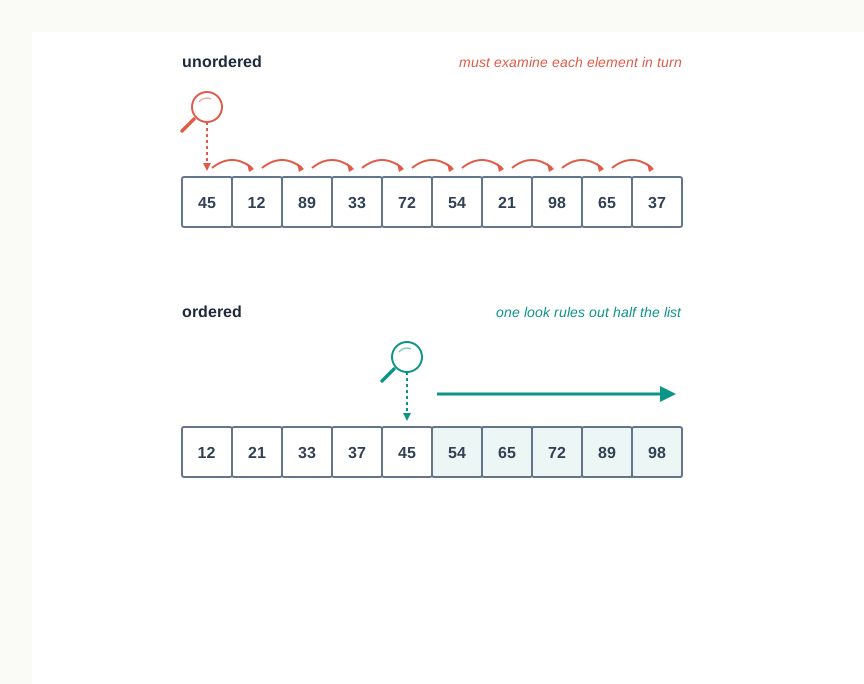
Fig. 5.1 – Searching ordered versus unordered data.
Ordering helps far beyond searching. Once a list is sorted, the smallest and the largest elements are simply the first and the last, and no scanning is needed to find them. Equal values come to lie next to each other, so duplicates can be detected by comparing neighbours. The median sits at the middle position. Two sorted lists can be merged into one sorted list in a single sweep. Printed output — a rank list, a fee-defaulters list, a stock report — is readable in a way that unordered output never is.
5.1.3 The Sort Key and the Order of Sorting
When a collection holds plain numbers, there is nothing to choose: the value of the element decides its position. Real data is rarely so simple. A record for a student carries a name, a roll number, a height and a set of marks, and any of these could decide the order. The field on whose value the ordering is decided is called the sort key.
Table 5.1 holds five records from a school sports register, printed in order of name.
The same five records ordered by height instead would run Ravi, Bhavna, Aarav, Meera, Ishaan. Nothing was added or removed — only the sort key changed, and with it the entire arrangement. This is why a specification such as “sort the list” is incomplete. A usable specification says what the key is and whether the order is ascending or descending.
Comparing Strings
Ordering names alphabetically works because Python can compare strings with the same operators used for numbers. Comparison proceeds character by character from the left; at the first position where the two strings differ, the character with the smaller underlying code decides the result. If one string runs out first and everything matched up to that point, the shorter string is treated as the smaller.
>>> "Anita" < "Bhavna"
True
>>> "anita" < "Bhavna"
False
The second result surprises most students. It is correct: in the character codes Python uses, every capital letter comes before every small letter, so "B" is smaller than "a" and the comparison is decided at the very first character. Alphabetical ordering in the everyday sense is recovered by comparing the strings in one consistent case.
Everything the three techniques in this chapter do rests on one comparison of the form “is this element greater than that one?” Change what that comparison means, and the same technique sorts by a different key or in the opposite order, without a single change to its structure.
5.1.4 Sorting as an Overhead Worth Paying
Sorting is not free. Elements must be compared with one another, and many of them must be moved, and for a large collection this takes a substantial amount of time. Time spent on work that is not the final answer, but that makes the final answer cheaper to obtain, is called overhead.
The question is whether the overhead is worth paying, and the honest answer is: it depends on how the sorted data will be used. Sorting a list to answer one question about it is usually wasteful, as the sidebar above showed. Sorting a list that will be searched a thousand times, printed as a report, checked for duplicates and merged with another list is an obvious bargain — the cost is paid once and recovered again and again.
This is exactly the calculation a school makes when it maintains its library register in order of accession number, or a shop makes when it keeps its stock ledger in order of item code. Somebody spends effort keeping the order; everybody who consults it afterwards spends less.
What This Chapter Covers
Because sorting is needed so widely, many different methods of doing it have been designed and studied, and computer scientists compare them by how their running time grows as the collection grows. A method for sorting, expressed as a definite sequence of steps, is called a sorting algorithm.
This chapter takes up three of them. Section 5.2 introduces bubble sort, which repeatedly compares neighbouring elements and exchanges them when they are out of order. Section 5.3 takes up selection sort, which finds the smallest remaining element and puts it directly where it belongs. Section 5.4 takes up insertion sort, which takes elements one at a time and slides each into its correct place among those already arranged. Each is stated first as an algorithm, then implemented in Python, then traced by hand on a small list so that you can see exactly what it does. Section 5.5 then asks the question that separates the three: how does the work grow when the list grows?
5.2 Bubble Sort
The first technique takes the simplest possible view of the problem. If a list is out of order, then somewhere in it there must be two neighbouring elements standing the wrong way round. Find such a pair, exchange them, and the list has become a little less disordered than it was. Keep doing that until no such pair is left, and the list must be sorted.
That single observation is the whole of bubble sort. Everything else is bookkeeping — deciding which pairs to check, in what order, and how to know when to stop.
5.2.1 Comparing Adjacent Elements and Swapping
Bubble sort never compares two elements that are far apart. It looks only at adjacent elements, that is, at a pair sitting in consecutive positions — the element at index j and the element at index j+1. If the first of the two is greater than the second, the two are swapped; otherwise nothing is done and the technique moves one step to the right.
Take the list [42, 17, 63, 9, 28], holding the marks of five students out of 70, and start at the left end. The elements at indices 0 and 1 are 42 and 17. Since \(42 > 17\), they are the wrong way round for ascending order, and they are exchanged, giving [17, 42, 63, 9, 28].
The comparison now moves one position right, to indices 1 and 2, which hold 42 and 63. These are already in order, so nothing happens. Then indices 2 and 3 hold 63 and 9, which are exchanged; then indices 3 and 4 hold 63 and 28, which are exchanged as well. The list has become [17, 42, 9, 28, 63].
Fig. 5.2 shows this sequence of comparisons step by step.
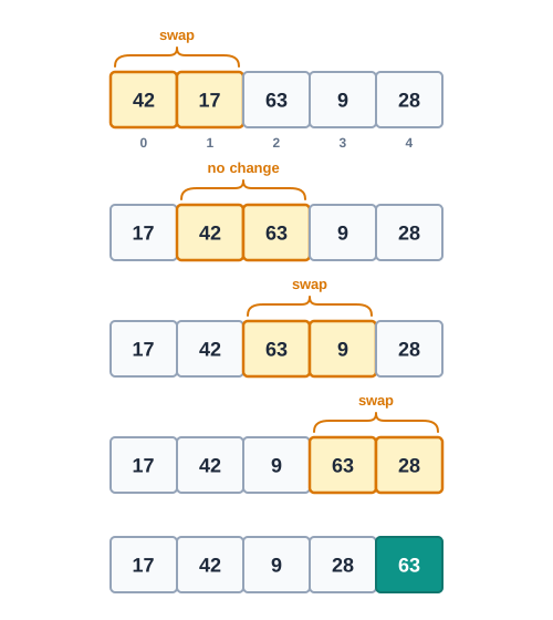
Fig. 5.2 – Step-by-step trace of the first pass of bubble sort.
Notice what happened to 63. It was compared at indices 2 and 3, won that comparison and moved right; it was compared again at indices 3 and 4, won again and moved right again. A large element, once met, is carried along to the right until something larger stops it — or until the end of the list is reached.
5.2.2 The Idea of a Pass
One complete sweep from the left end of the list to the point where the comparisons stop is called a pass. The four comparisons just made — at index pairs (0,1), (1,2), (2,3) and (3,4) — form the first pass over a five-element list.
A single pass does not sort the list, and it is not meant to. What it guarantees is much narrower and much more useful: at the end of the first pass, the largest element of the list is standing in the last position. In the example above, 63 finished at index 4, and that is where it belongs in the final answer.
Because that position is now correct and will never need to change, the next pass need not look at it. The second pass therefore examines only the first four elements, the third pass only the first three, and so on. The region still being worked on shrinks by one element after every pass.
5.2.3 How the Largest Element Bubbles Up
The reason a pass always deposits the largest element at the end is worth stating carefully, because it is the correctness argument for the whole method. Consider the largest element of the list, wherever it happens to be. The moment the sweep reaches it, that element is compared with its right-hand neighbour. Being the largest, it is greater than that neighbour, so a swap occurs and it moves one place right. The sweep also moves one place right, so the very next comparison involves the same element again. It therefore keeps winning and keeps moving until the sweep runs off the end of the list — and there is nowhere for it to stop except the last position.
This steady rise of the largest value to the top of the list is the image that gives the technique its name: the value behaves like a bubble rising through water. The remaining elements are not left untouched in the meantime. Every out-of-order neighbouring pair the sweep happens to meet is corrected on the way, so the list ends each pass in better shape than it began.
Continuing the example, the second pass works on [17, 42, 9, 28, 63] but ignores the settled 63. It compares 17 with 42 and leaves them; swaps 42 and 9; swaps 42 and 28. The list becomes [17, 9, 28, 42, 63], and 42 has settled into the second-last position.
The third pass works on the first three elements. It swaps 17 and 9, then leaves 17 and 28 alone, giving [9, 17, 28, 42, 63]. The list is now sorted, although the technique as stated does not yet know that. Fig. 5.3 shows the state of the list at the end of each pass, with the settled tail growing from the right.
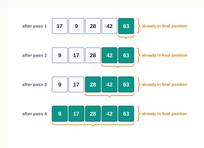
Fig. 5.3 – The list at the end of each pass of bubble sort.
5.2.4 Algorithm for Bubble Sort
The method can now be written as a definite sequence of steps. Two counters are needed: one, i, to count the passes, and another, j, to walk across the list within a pass. The inner walk must stop before the settled tail, which after i completed passes holds i elements — hence the limit \(n-i-1\).
Only \(n-1\) passes are needed, not \(n\). Each pass settles one element, so after \(n-1\) of them exactly one element remains unsettled, and a single element compared with nothing is already in order. A list of five elements is therefore sorted in four passes.
5.2.5 Implementing Bubble Sort in Python
Translating the algorithm into Python is direct. The two WHILE loops become for loops over ranges, because in both cases the number of repetitions is known in advance. range(n - 1) produces the pass numbers \(0, 1, \dots, n-2\), and range(n - 1 - i) produces the index positions examined during pass i.
5.2.6 Counting the Passes and the Comparisons
How much work has been done? The first pass over a list of \(n\) elements makes \(n-1\) comparisons, the second makes \(n-2\), and so on down to the last pass, which makes a single comparison. Table 5.3 sets this out for the five-element list traced above.
Adding the column gives the total number of comparisons for any list of \(n\) elements:
\[(n-1) + (n-2) + \cdots + 2 + 1 = \frac{n(n-1)}{2}\]
For \(n = 5\) this is \(\frac{5 \times 4}{2} = 10\), which matches the trace exactly. The important feature of this expression is not its precise value but how it grows: doubling the number of elements multiplies the comparisons by roughly four. Section 5.5 returns to this point.
The number of comparisons is fixed — it does not depend on the data at all. The number of swaps does. A list that is already in ascending order needs no swaps whatsoever; this is the best case. A list arranged in exactly descending order needs a swap at every single comparison, giving \(\frac{n(n-1)}{2}\) swaps; this is the worst case. Ordinary unsorted data falls somewhere between the two.
5.2.7 Detecting a List That Is Already Sorted
The dry run exposed an obvious waste. The list was fully sorted at the end of pass 2, yet pass 3 ran anyway, because the loop was told to make \(n-1\) passes and it obediently made them.
There is a clean signal available. If an entire pass completes without performing a single swap, then no adjacent pair was out of order — and a list in which no adjacent pair is out of order is, by definition, sorted. The moment such a pass occurs, the remaining passes can only repeat the same finding, so the work can stop.
The signal is recorded in an ordinary variable used as a flag: a variable whose value stands for a yes-or-no fact about what has happened. It is set to False at the start of each pass and turned to True the instant a swap takes place. After the pass, its value answers the question “did anything move?”
5.2.8 Sorting in Descending Order
Nothing in bubble sort assumes that smaller elements belong on the left. That assumption lives in exactly one place — the condition inside the if statement — and reversing it reverses the sorted order.
To sort in descending order, an element should move right when it is smaller than its neighbour. The comparison data[j] > data[j + 1] therefore becomes data[j] < data[j + 1], and now it is the smallest element that is carried to the end of the list in each pass.
def bubble_sort_desc(data):
    n = len(data)
    for i in range(n - 1):
        for j in range(n - 1 - i):
            if data[j] < data[j + 1]:
                data[j], data[j + 1] = data[j + 1], data[j]

scores = [55, 12, 70, 33]
bubble_sort_desc(scores)
print(scores)
[70, 55, 33, 12]The structure of the loops, the number of passes and the number of comparisons are all unchanged. This is a general point about sorting techniques, and it is worth carrying forward to the next two sections: the technique decides how elements are moved about, while a single comparison decides what counts as being in order. Change the comparison and you change the ordering; change nothing else.
5.3 Selection Sort
Bubble sort works by correcting local mistakes: it keeps fixing neighbouring pairs and trusts that the list will come into order as a result. It reaches the right answer, but it moves elements about a great deal on the way — a single element may be picked up and put down again in pass after pass.
The next technique takes the opposite view. Instead of nudging elements towards their positions, it decides a position outright and fills it once, correctly, and never touches it again. This is selection sort, so called because each pass selects the element that belongs in the next position.
5.3.1 Dividing the List into a Sorted and an Unsorted Part
Think of the list as being split into two regions by an imaginary line. Everything to the left of the line is finished: those elements are in their final positions and in the correct order. Everything to the right is still unexamined. Initially the line sits at the very beginning, so the finished region is empty and the unfinished region is the whole list.
Each pass moves the line one position to the right. To do that, the pass must work out which of the remaining elements deserves the position immediately to the right of the line — and for ascending order, that is the smallest element of the unfinished region.
Fig. 5.4 shows the first pass on the list [35, 12, 48, 20, 27], holding five bus fares in rupees.
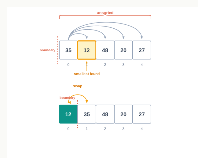
Fig. 5.4 – The first pass of selection sort.
Notice how differently this behaves from bubble sort. There, an element crept one position at a time. Here, 12 travelled from index 1 to index 0 in a single move, and it could just as easily have travelled from index 4 to index 0 in the same single move. Selection sort does not care how far an element has to go.
5.3.2 Selecting the Smallest Element in Each Pass
Finding the smallest element of the unfinished region is a small task in its own right, and it is worth stating on its own because it is used constantly in programming. You cannot know the smallest value without looking at every candidate, so the region is scanned from left to right while a record is kept of the best value seen so far.
In practice it is the position of the smallest element that is recorded, not the value. The position is what the swap will need, and from the position the value can always be recovered by indexing.
So the pass proceeds like this. Assume, to begin with, that the leftmost unfinished element is the smallest, and remember its index. Compare each later element with the element at the remembered index; whenever a smaller one appears, forget the old index and remember the new one. When the scan reaches the end of the list, the remembered index is certainly the position of the smallest element, because every element was compared against the best candidate available at the time.
Then one swap puts that element where it belongs, and whatever was occupying that position is displaced into the gap left behind. It is still in the unfinished region, so it will be considered again later.
Continuing the fares example, the second pass scans indices 1 to 4 of [12, 35, 48, 20, 27] and finds 20 to be the smallest, so 20 and 35 are exchanged, giving [12, 20, 48, 35, 27]. The third pass scans indices 2 to 4, finds 27, and exchanges it with 48, giving [12, 20, 27, 35, 48]. The fourth pass scans indices 3 to 4, finds that 35 is already the smaller of the two, and does nothing at all. Fig. 5.5 shows the boundary advancing across the list.
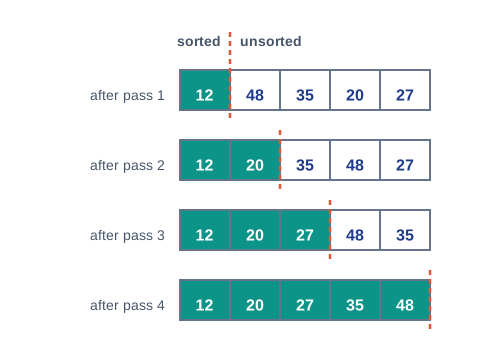
Fig. 5.5 – The list at the end of each pass of selection sort.
5.3.3 Algorithm for Selection Sort
Two counters are needed again. The outer counter i marks the boundary — it is the position being filled in this pass. The inner counter j scans the unfinished region, which runs from i+1 to the end of the list. A third variable holds the index of the smallest element found so far.
Only \(n-1\) passes are needed here as well, and for the same reason as before: once \(n-1\) positions have been filled correctly, the single element left over has no other place to be.
5.3.4 Implementing Selection Sort in Python
The inner scan is written as range(i + 1, n), which is Python’s way of saying “from the position just after the boundary up to the end of the list”. Both loop limits change from pass to pass, and both depend on i.
5.3.5 Comparisons and Swaps in Selection Sort
The first pass compares the leftmost unfinished element with \(n-1\) others, the second with \(n-2\) others, and so on, down to a single comparison in the last pass. The total is therefore
\[(n-1) + (n-2) + \cdots + 1 = \frac{n(n-1)}{2}\]
which for the five fares gives \(\frac{5 \times 4}{2} = 10\) — exactly the number of rows in the dry run above, and exactly the same count that bubble sort needed for a list of five.
What is striking is that this count is completely fixed. Selection sort has no idea whether the list handed to it is already sorted, badly jumbled or perfectly reversed, and it performs the same ten comparisons in every case. There is no best case and no worst case to speak of, and no flag can rescue it, because a pass that finds nothing to move has still had to look at everything to be sure.
The exchanges tell a different story. Each pass performs at most one, so a list of \(n\) elements needs at most \(n-1\) exchanges however disordered it is — and often fewer, as the trace showed with three. Compare that with bubble sort, which on a reversed list performs \(\frac{n(n-1)}{2}\) exchanges. For a list of 100 elements, that is at most 99 exchanges against as many as 4,950.
5.3.6 Bubble Sort and Selection Sort Contrasted
The two techniques are close relatives. Both work in place, both need no second list, both make the same number of comparisons, and both settle one element per pass. The differences lie in which element gets settled, and in how much data has to move to settle it.
Read the fifth row carefully, because it is the practical difference between the two. Comparing two values is cheap. Moving data can be expensive — if each element were a long record rather than a number, every exchange would mean copying a great deal of memory. Selection sort was designed for exactly that situation: it spends comparisons freely in order to keep exchanges to a minimum.
5.4 Insertion Sort
Watch somebody arrange a hand of playing cards. They do not scan the whole hand looking for the smallest card, and they do not repeatedly swap neighbouring cards. They pick up one card at a time, look along the cards already held, and push it into the gap where it belongs — sliding the others aside to make room.
That is insertion sort, and of the three techniques in this chapter it is the one closest to how people actually order things by hand.
5.4.1 Placing Each Element Where It Belongs
Like selection sort, insertion sort keeps the list divided into a finished region on the left and an unfinished region on the right. The resemblance ends there, and the difference matters.
In selection sort, the left region held elements that were in their final positions — an element placed there was never moved again. In insertion sort the left region holds elements that are in order among themselves, but not necessarily in their final positions. An element sitting comfortably at index 0 may well be pushed to index 1 later, when something smaller turns up.
The technique starts with a finished region of exactly one element. A single element, having nothing to be out of order with, is trivially in order. Every pass then takes the first element of the unfinished region and inserts it into its correct place among the elements on the left, which enlarges the ordered region by one.
Take the list [46, 15, 39, 8, 22], holding the runs scored by five players in a match. The ordered region begins as [46] and the first element to be placed is 15. Since \(15 < 46\), it belongs before 46, so 46 moves one position right and 15 takes its place: [15, 46, 39, 8, 22].
5.4.2 Shifting Elements to Make Space
Making room is where insertion sort does its real work, and it is done by shifting rather than swapping. To shift an element is to copy it into the position immediately to its right, one element at a time, so that a gap opens up where the new element can be written.
The order of operations here needs care. Before anything is shifted, the element being placed must be copied into a separate variable — conventionally called temp — because the very first shift will overwrite the position it was occupying. With the value safely held, the scan can walk leftwards through the ordered region, shifting each element that is larger than temp one place right, and stopping the moment it meets an element that is not larger, or runs off the left end of the list. Whatever position the scan has vacated is then where temp is written.
Fig. 5.6 shows this happening for the value 8, the fourth element of the example list.
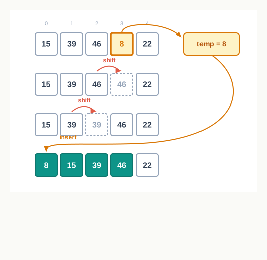
Fig. 5.6 – Shifting elements to insert a value into the ordered region.
Three elements moved right, and then 8 was written into the vacated position at index 0. Notice that only one value entered the list from outside — the one held in temp — while everything else simply slid along. A swap-based method would have needed three separate exchanges to achieve the same thing, each involving two writes instead of one.
Continuing to the last element, 22 is held in temp; 46 and 39 are both larger and shift right; 15 is not larger, so the scan stops there and 22 is written into the gap at index 2, giving [8, 15, 22, 39, 46]. Fig. 5.7 shows the ordered region growing across the four passes.
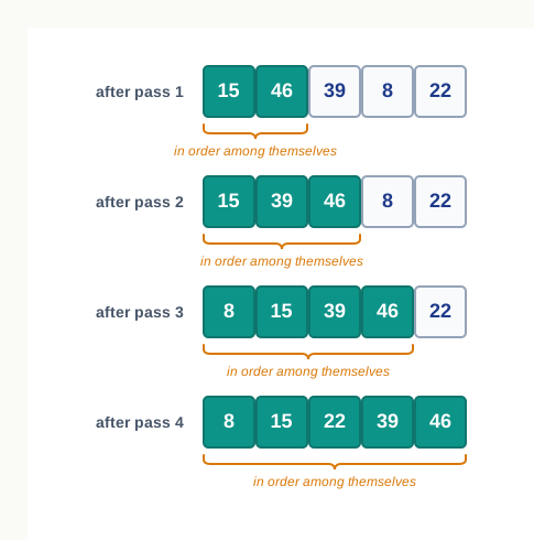
Fig. 5.7 – The list at the end of each pass of insertion sort.
5.4.3 Algorithm for Insertion Sort
The outer counter i marks the element currently being placed, and it starts at 1 rather than 0, because the element at index 0 already forms the initial ordered region. The inner counter j walks leftwards from i-1, and it must stop for either of two reasons — running past the left end of the list, or meeting an element that is not larger than the value being inserted.
The condition in Step 5 has two parts joined by AND, and the order in which they are written is not arbitrary. j >= 0 must be tested first, because the second test reads numList[j] and that reading is only meaningful while j is a valid index.
5.4.4 Implementing Insertion Sort in Python
The inner loop is written as a while rather than a for, because the number of repetitions is not known in advance — it depends entirely on how far leftwards the value has to travel. This is the first of the three techniques whose inner loop can finish early.
The duplicated values that appear in the middle rows of the trace are not errors. During a shift the same value genuinely occupies two positions for a moment, and the copy left behind is overwritten either by the next shift or by the final write of temp.
5.4.5 Behaviour on Nearly Sorted and Reversed Lists
Insertion sort is the first technique in this chapter whose work depends heavily on the data it is given, and the dependence is worth understanding because it decides when the technique should be chosen.
Suppose the list is already in ascending order. Every pass makes exactly one comparison, finds the value already larger than its left neighbour, shifts nothing, and ends. For \(n\) elements that is \(n-1\) comparisons and no shifting whatever — the best case, and it is remarkably cheap. Selection sort on the same list would still grind through all \(\frac{n(n-1)}{2}\) comparisons.
Now suppose the list is in exactly reverse order. Every element being inserted is smaller than everything to its left, so every pass scans the entire ordered region and shifts every element in it. The \(i\)-th pass then makes \(i\) comparisons, and the total climbs to \(\frac{n(n-1)}{2}\) — the worst case, and no better than the other two techniques.
Between these extremes lies the case that matters in practice. Data is often nearly sorted: a fresh set of marks appended to a sorted list, a register with a few late entries, a file that was sorted last week and has since had a handful of additions. In such a list each element has only a short distance to travel, so each pass stops after a couple of comparisons, and insertion sort finishes far faster than its worst case suggests.
5.4.6 Sorting Data as It Arrives
There is one situation the other two techniques cannot handle gracefully at all, and insertion sort handles naturally. Suppose the data does not exist as a complete list to begin with. Names are entered at an admission counter one at a time, readings arrive from an instrument through the day, entries are added to a register as visitors sign in — and the collection must be in order after every addition, not only at the end.
Bubble sort and selection sort both assume the whole list is present before they begin. Insertion sort makes no such assumption. Its every pass is already an “insert one more element into an ordered list” operation, so a single pass, run once per arrival, keeps the list permanently in order.
5.5 Time Complexity of Algorithms
Three techniques have now been studied, and all three do the job. On a list of five elements they finish in a fraction of a second and there is nothing to choose between them. The chapter opened with a warning that this comfort does not last: what is invisible at five elements can decide everything at ten lakh.
This section supplies the tool for saying so precisely. It is a way of describing how the work an algorithm does grows as the amount of data grows — and it is the reason computer scientists design new sorting techniques even though the old ones are perfectly correct.
5.5.1 Why the Same Task Has Faster and Slower Solutions
You have met this idea before. In Class XI, several different algorithms were compared for deciding whether a number is prime: testing every divisor from 2 up to \(n-1\), stopping at \(n/2\), stopping at \(\sqrt{n}\). All of them give the same verdict on every number. They differ only in how much work they do to reach it, and on a large number the difference is glaring.
Sorting is the same story with higher stakes, because sorting is applied to whole collections rather than to single values. A problem can always be solved in more than one way, and the ways are not equally cheap.
The obvious way to compare two solutions would be to run both and time them with a clock. That measurement is almost useless, because it describes the machine as much as the algorithm. Run the same program on a newer computer and every timing improves; run it while other programs are busy and every timing worsens. What is needed is a measure that belongs to the algorithm itself.
The measure used is the number of basic operations performed, counted as a function of the amount of data. For a sorting technique the basic operation is the comparison of two elements, and the amount of data is the number of elements, written \(n\). That count does not change when the computer changes, and it is exactly what was being worked out in Table 5.3 and in section 5.3.5.
5.5.2 What Time Complexity Measures
The amount of time an algorithm takes to process the data given to it is called its time complexity, and it is expressed not as a number of seconds but as an expression in \(n\).
Read the definition carefully, because it is easy to want more from it than it offers. Time complexity does not tell you how long a program will take. It tells you what happens to the running time when the input grows — whether doubling the data doubles the work, or quadruples it, or leaves it untouched. That is a coarse statement, and it is deliberately coarse, because the coarse statement is the one that survives a change of machine.
For small collections the distinction hardly registers. Every technique in this chapter sorted five elements instantly, and so would a considerably worse one. It is when a program built for ten records meets ten lakh records that the shape of the growth decides whether an answer arrives in a moment, arrives after lunch, or never arrives at all.
Working out complexity exactly involves mathematics beyond this book. What can be done here — and what is genuinely useful — is to estimate it by looking at the structure of the loops in the code.
5.5.3 Estimating Complexity by Reading the Loops
The estimate rests on a simple observation: statements that are executed once contribute almost nothing, while statements inside a loop contribute once for every repetition of that loop. So the complexity of a piece of code is decided by its loops, and by how they are arranged.
Four guidelines cover everything in this chapter.
- Code with no loop at all performs a fixed number of steps, whatever the size of the data. Its time complexity is constant.
- A single loop that runs from beginning to end of the data performs its body \(n\) times, so its complexity is \(n\).
- A loop inside another loop performs its body up to \(n\) times for each of \(n\) repetitions of the outer loop, so its complexity is \(n^2\).
- When code contains a nested loop and also a separate single loop, the nested loop decides the estimate. For large \(n\) the term \(n^2\) dwarfs the term \(n\), so adding the smaller term changes nothing worth recording.
5.5.4 Constant, Linear and Quadratic Time
Three names cover the algorithms met in this chapter, and each deserves a concrete example.
Constant time
def midpoint_of_range(data):
    return (data[0] + data[-1]) / 2
This function does the same three or four operations whether data holds five elements or five lakh, because it never looks at anything except the two ends. Its running time does not grow with \(n\) at all, and such an algorithm is called a constant time algorithm.
Linear time
def count_above(data, limit):
    count = 0
    for value in data:
        if value > limit:
            count = count + 1
    return count
Here the body of the loop runs once per element, so the work is proportional to \(n\). Doubling the number of elements doubles the work. This is a linear time algorithm, and finding the largest value, adding up a list and searching an unordered list for a value are all of this kind.
Quadratic time
def count_pairs(data, total):
    n = len(data)
    pairs = 0
    for i in range(n):
        for j in range(i + 1, n):
            if data[i] + data[j] == total:
                pairs = pairs + 1
    return pairs
This function counts the pairs of elements that add up to a given total — on the list [10, 20, 30, 40] with a total of 50 it returns 2, since 10 with 40 and 20 with 30 both qualify. Every element is combined with every later element, so the comparison runs about \(\frac{n^2}{2}\) times. Doubling the data multiplies the work by roughly four, and such an algorithm is called a quadratic time algorithm.
Fig. 5.8 shows what these three growth patterns look like when drawn side by side.
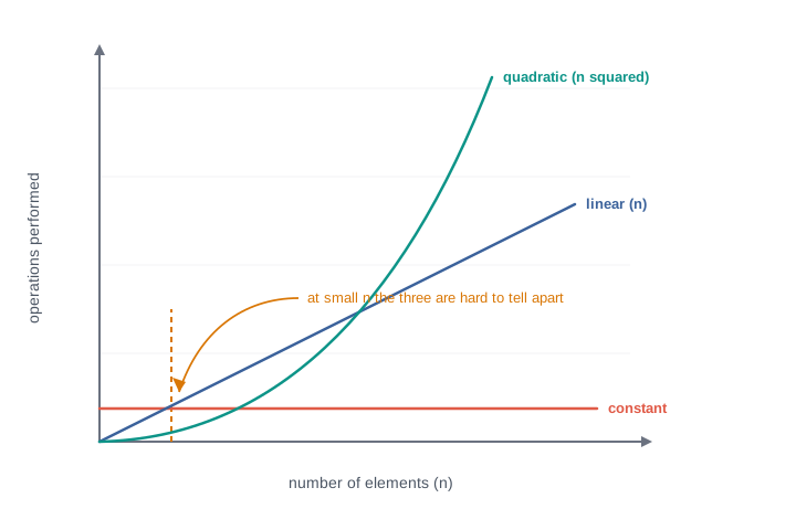
Fig. 5.8 – Growth rates of constant, linear, and quadratic time algorithms.
The dashed line in the figure carries the practical lesson. Near the left edge the three curves are almost on top of one another, which is exactly why a badly chosen algorithm behaves perfectly well in testing on ten records. Move right and they separate without limit.
5.5.5 Complexity of the Three Sorting Techniques
Now look back at the three programs written in this chapter. In bubble_sort, a for loop over j sits inside a for loop over i. In selection_sort, a for loop over j sits inside a for loop over i. In insertion_sort, a while loop over j sits inside a for loop over i. All three have a loop within a loop, so by the third guideline all three are quadratic time algorithms, with a time complexity of \(n^2\).
This agrees exactly with the counts worked out earlier by hand. Both bubble sort and selection sort make \(\frac{n(n-1)}{2}\) comparisons, and multiplying that out gives \(\frac{n^2 - n}{2}\) — an expression whose largest term is \(n^2\).
The estimate is deliberately blunt. It ignores the division by 2, and it ignores the \(-n\), because neither changes what happens as \(n\) grows large. Two algorithms that both take about \(n^2\) steps may still differ by a constant factor, and that factor is worth having; but it is a smaller matter than the shape of the curve, and it is the shape that the complexity records.
Table 5.10 makes the consequence concrete for \(\frac{n(n-1)}{2}\) comparisons. The last column assumes a machine that performs \(10^8\) comparisons per second, which is the right order of magnitude for an ordinary computer.
Read the table downwards. Each row multiplies the number of elements by ten, and each row multiplies the work by roughly a hundred. That is the signature of quadratic growth, and it is why a program that sorts a class list of forty names in no time at all can be entirely unusable on a list of ten lakh.
One qualification belongs here. Insertion sort’s inner while loop does not always run to completion — on a list already in order it stops after a single comparison, giving \(n-1\) comparisons in all, which is linear. Its quadratic label describes its worst case, not every case. Selection sort has no such escape: its inner loop is a for over a fixed range and runs fully every time, whatever the data.
5.5.6 Choosing a Technique for a Given Situation
Since all three techniques are quadratic, complexity alone cannot separate them. The separation comes from how each behaves on particular kinds of data, and from whether comparing or moving is the expensive operation in the situation at hand.
Three readings of this table are worth carrying away. If the data is likely to be already ordered or nearly so, insertion sort — or bubble sort with the early stop — does very little work, while selection sort does all of it regardless. If each element is a bulky record and copying it is expensive, selection sort’s promise of at most \(n-1\) exchanges is valuable. And if the elements arrive one at a time rather than all at once, insertion sort is the only one of the three that fits at all.
The final reading is the widest one. All three are quadratic, so for genuinely large collections none of them is the right answer, and Python’s own sorting facilities — built on techniques beyond this book — should be used instead. What these three teach is not a toolkit for large data. It is the habit of asking, of any program you write, how its work grows when its input does.
5.6 Summary
Sorting and Why It Is Done
Sorting is the process of rearranging the elements of a collection so that they appear in a specified order. No element is added, removed or altered; only positions change.
Numbers may be arranged in ascending order, running from the smallest value to the largest, or in descending order, running from the largest down to the smallest. Strings may be ordered alphabetically or by length.
The value on which the ordering is decided is called the sort key. The same collection produces entirely different arrangements under different keys, so an instruction to sort is incomplete until the key and the direction are stated.
Ordered data makes later work cheaper: searching becomes faster, the smallest and largest elements sit at the two ends, duplicates come to lie next to each other, and two ordered lists can be merged in a single sweep.
Sorting itself costs time, and time spent making later work cheaper is called overhead. It is worth paying when the ordered collection will be used repeatedly, and wasteful when a single fact is wanted once.
Because a list is mutable, all three techniques in this chapter rearrange the original list in place rather than building a second one. Exchanging two elements is done in a single statement so that neither value is overwritten before it is read.
Bubble Sort
Bubble sort compares adjacent elements only, and swaps a pair whenever the left element is greater than the right one.
One complete traversal of the region under consideration is called a pass. A pass guarantees that the largest element of that region finishes at its right end, because the sweep keeps pushing that element rightwards.
Each pass settles one element, so the region examined shrinks by one after every pass, and \(n-1\) passes are enough for a list of \(n\) elements.
A small element moves left by only one position per pass, which is why many passes are needed even though a large element can travel a long way in one.
The technique makes \(\frac{n(n-1)}{2}\) comparisons. The number of swaps depends on the data: none in the best case, when the list is already ordered, and one at every comparison in the worst case, when the list is exactly reversed.
A pass that performs no swap proves that the list is already sorted. Recording that fact in a flag variable, reset at the start of every pass, allows the remaining passes to be abandoned.
Reversing the comparison inside the decision reverses the sorted order. The structure of the loops and the number of comparisons do not change.
Selection Sort
Selection sort keeps the list divided by a boundary: everything to the left is in its final position, everything to the right is still unexamined.
Each pass scans the unsorted region for the smallest element, remembering its position rather than its value, and then exchanges that element with the leftmost element of the region. The boundary advances by one position.
The decision is taken first and the data is moved once, at the end of the pass, so an element travels any distance in a single exchange.
The number of comparisons is \(\frac{n(n-1)}{2}\) regardless of the data, so the technique cannot recognise a list that is already ordered and cannot stop early.
At most \(n-1\) exchanges are performed, which makes selection sort attractive when moving an element is expensive.
Insertion Sort
Insertion sort treats the first element as an ordered region of one, then takes each remaining element in turn and inserts it into that region at its correct place.
The elements in the ordered region are in order among themselves, but not necessarily in their final positions; an element already placed may be pushed rightwards later.
Space is made by shifting rather than swapping: each element greater than the value being inserted is copied one position right, and the value is then written into the vacated position.
The value being inserted must be copied into a temporary variable before any shifting begins, because the first shift overwrites the position it occupied.
The inner scan stops for either of two reasons — reaching the left end of the list, or meeting an element that is not greater than the value being inserted. The index must be checked before the element at that index is read.
On an already ordered list the technique makes only \(n-1\) comparisons and shifts nothing; on a reversed list it makes \(\frac{n(n-1)}{2}\) comparisons and shifts at every one.
Because each pass is itself an insertion into an ordered list, the technique can keep a collection in order while data is still arriving, one insertion per new element. The other two techniques require the whole collection to be present before they begin.
Time Complexity of Algorithms
The time complexity of an algorithm describes how the number of operations it performs grows with the size of the input, expressed in terms of that size. It is not a measurement in seconds, and it does not change when the machine changes.
Complexity is estimated from the structure of the loops. Code with no loop is constant time; a single loop over the data is linear time, written \(n\); a loop within a loop is quadratic time, written \(n^2\).
Where a nested loop and a separate single loop both occur, the nested loop decides the estimate, since for large inputs the larger term dominates.
All three sorting techniques in this chapter contain a loop within a loop, so all three are quadratic time algorithms with a time complexity of \(n^2\).
Quadratic growth means that multiplying the number of elements by ten multiplies the work by about a hundred. This is why the choice of technique is invisible on a few dozen records and decisive on several lakh.
The quadratic label describes the worst case. Insertion sort behaves linearly on data that is already nearly in order, whereas selection sort performs the same comparisons whatever it is given.
Since all three grow quadratically, none of them is the right choice for very large collections. What they teach is the habit of asking how a program’s work grows when its input does.
5.7 Key Terms
Adjacent elements — two elements of a list occupying consecutive positions, such as the elements at index
jand indexj+1.Ascending order — an arrangement in which each element is smaller than or equal to the one after it, so the collection runs from the smallest value to the largest.
Best case — the arrangement of input data on which an algorithm does the least work; for bubble sort and insertion sort, a list already in the required order.
Bubble sort — a sorting technique that repeatedly compares adjacent elements and swaps them when they are out of order, so that the largest element of the unsorted region reaches its right end in each pass.
Constant time — the behaviour of an algorithm whose number of operations does not grow at all as the input grows, because it contains no loop over the data.
Descending order — an arrangement in which each element is greater than or equal to the one after it, so the collection runs from the largest value to the smallest.
Flag — a variable whose value records a yes-or-no fact about what has happened, such as whether any swap occurred during a pass.
Insertion sort — a sorting technique that takes each element in turn and inserts it into its correct place among the elements already in order, shifting larger elements one position right to make room.
Linear time — the behaviour of an algorithm whose number of operations grows in proportion to the size of the input, produced by a single loop over the data.
Mutable — the property of a list that allows an element to be replaced by assigning to its index, so that the list changes without a new list being created.
Overhead — time spent on work that is not the final answer but that makes the final answer cheaper to obtain, such as the time spent sorting before searching.
Pass — one complete traversal of the region of a list under consideration, during which every required pair of elements is examined once.
Quadratic time — the behaviour of an algorithm whose number of operations grows as the square of the input size, produced by a loop nested within another loop.
Selection sort — a sorting technique that scans the unsorted region for its smallest element and exchanges that element with the leftmost element of the region, advancing the boundary by one position each pass.
Shifting — copying an element one position to the right within the same list so as to vacate a position for another element; it moves one element, unlike a swap, which exchanges two.
Sort key — the value, drawn from each element, that is used to decide that element’s position in the sorted order.
Sorting — the process of rearranging the elements of a collection so that they appear in a specified order, without adding, removing or altering any element.
Sorting algorithm — a definite sequence of steps that arranges the elements of a collection into the required order.
Swap — to exchange two elements so that each takes the other’s position, done in Python in a single assignment statement.
Time complexity — a description of how the number of operations an algorithm performs grows with the size of its input, expressed in terms of that size rather than in seconds.
Worst case — the arrangement of input data on which an algorithm does the most work; for all three techniques of this chapter, a list arranged in exactly the reverse of the required order.
5.8 Points to Ponder
Bubble sort with a flag can discover in a single pass that a list is already in order, while selection sort scans every element every time and can never make that discovery. Yet selection sort is the one recommended when each element is a bulky record. What does this suggest about calling one algorithm “more efficient” than another without saying what is being counted?
Bubble sort and selection sort make exactly the same number of comparisons for a list of \(n\) elements. If the comparison count is identical, what did the second technique actually contribute, and would you call it a genuinely different idea or the same idea rearranged?
In selection sort an element placed in the sorted region never moves again; in insertion sort an element already placed may be pushed rightwards many times before the work ends. Insertion sort nevertheless finishes with the same correct list. Which of the two guarantees is worth more, and to whom — the person writing the program, or the machine running it?
Time complexity deliberately discards the division by 2 and the \(-n\) in \(\frac{n(n-1)}{2}\), keeping only \(n^2\). Something true is being thrown away on purpose. What is gained by the discarding, and can you describe a situation in which the discarded detail would have mattered?
A quadratic technique sorting ten lakh records takes over an hour on an ordinary machine. Suppose a computer ten times faster were available. Would that be a fair solution to the problem, and what would happen the following year when the data grew to a crore?
Sorting a list is expensive; searching a sorted list is cheap. For a collection that will be searched some number of times, there must be a point at which sorting first begins to pay for itself. How would you go about estimating where that point lies, and what would you need to know about the data to do it?
5.9 Objective Questions
A list of 12 elements is to be sorted using bubble sort, written without any early termination. How many passes will be made over the list?
- 10
- 11
- 12
- 13 [1 mark]
Which of the following techniques performs at most
n - 1exchanges on a list ofnelements, whatever the starting arrangement?- Bubble sort
- Selection sort
- Insertion sort
- All three perform at most
n - 1exchanges [1 mark]
An algorithm contains a loop written inside another loop, each running over the whole data. Its time complexity is estimated as
- constant
- \(n\)
- \(2n\)
- \(n^2\) [1 mark]
In the following question, an Assertion (A) is followed by a Reason (R). Choose the correct option. Assertion (A): In insertion sort, the element being inserted is copied into a temporary variable before any shifting begins. Reason (R): The first shift writes into the position that the element was occupying.
- Both A and R are true, and R is the correct explanation of A.
- Both A and R are true, but R is not the correct explanation of A.
- A is true but R is false.
- A is false but R is true. [1 mark]
In the following question, an Assertion (A) is followed by a Reason (R). Choose the correct option. Assertion (A): Selection sort makes fewer comparisons when the list handed to it is already in ascending order. Reason (R): The inner loop of selection sort runs over a fixed range and is completed in every pass.
- Both A and R are true, and R is the correct explanation of A.
- Both A and R are true, but R is not the correct explanation of A.
- A is true but R is false.
- A is false but R is true. [1 mark]
Fill in the blank: In bubble sort, one complete traversal of the region of the list under consideration is called a ____________. [1 mark]
State whether true or false: In insertion sort, an element that has been placed in the ordered region never changes its index again. [1 mark]
Match each item in Column A with the correct item in Column B.
| Column A | Column B |
|---|---|
| a. Code containing no loop over the data | i. Linear time |
| b. A single loop running over the whole data | ii. Selection sort |
| c. A loop written within another loop | iii. Constant time |
| d. An element moving any distance in one exchange | iv. Quadratic time |
[1 mark]
5.10 Check Your Concepts
Define sorting. State one reason why a collection that will be searched many times is sorted first. [2 marks]
Differentiate between shifting and swapping as used in this chapter, in two points. [2 marks]
Using the list
[30, 10, 20], show what one complete pass of bubble sort produces, and explain why the largest element of a region must finish at the right end of that region. [3 marks]For a list of 6 elements, state the number of comparisons made by each of the following, and justify each answer in one line:
- selection sort, on any arrangement of the data
- insertion sort, on a list already in ascending order
- bubble sort written without early termination [3 marks]
Write a user-defined function that arranges a list of integers in descending order using bubble sort, abandoning the remaining passes as soon as a pass performs no swap. Explain in two lines why the flag must be set to
Falseat the start of every pass rather than once before the outer loop. [4 marks]Readings from an instrument arrive one at a time through the day, and the list of readings must be in ascending order after every arrival.
- Name the sorting technique this situation corresponds to, and justify the choice in one line.
- Write a user-defined function that inserts one new reading into an already ascending list.
- Give the reasoning that shows your function leaves the list in ascending order.
- State one kind of input on which this technique performs badly. [5 marks]
5.11 Output & Debugging
- Predict the output of the following code, and state how many swaps take place.
data = [5, 2, 9, 1]
n = len(data)
for j in range(n - 1):
    if data[j] > data[j + 1]:
        data[j], data[j + 1] = data[j + 1], data[j]
print(data)
[2 marks]
- The following program is meant to sort the list in ascending order using selection sort, but it does not.
def sort_list(data):
    n = len(data)
    for i in range(n - 1):
        min_pos = i
        for j in range(i + 1, n):
            if data[j] < data[min_pos]:
                min_pos = j
                data[i], data[min_pos] = data[min_pos], data[i]

values = [4, 1, 3]
sort_list(values)
print(values)
State the output the program actually produces, identify the single error, and write the corrected program. [3 marks]
- State the value printed by the following code, and say in one line what the printed value represents for a list of six elements.
data = [12, 7, 25, 3, 18, 6]
count = 0
n = len(data)
for i in range(n - 1):
    for j in range(n - 1 - i):
        count = count + 1
print(count)
[2 marks]
- Give the output of the following code. Also state the value held by
jat the moment thewhileloop stops during the last repetition of the outer loop.
data = [20, 35, 15, 40, 10]
for i in range(1, 3):
    temp = data[i]
    j = i - 1
    while j >= 0 and data[j] > temp:
        data[j + 1] = data[j]
        j = j - 1
    data[j + 1] = temp
print(data)
[3 marks]
5.12 Case-Based Questions
- A school library records how many times each of six books was issued during a month. The counts are held in a list, in the order in which the books appear on the shelf:
issues = [14, 3, 27, 9, 21, 6]The librarian wants the list rearranged in descending order, so that the most frequently issued books can be identified at a glance, and has decided to use bubble sort. a. State the single change that must be made to an ascending bubble sort function to obtain descending order. [1 mark] b. Show the contents of the list at the end of the first complete pass, and mark the element that has reached its final position. [2 marks] c. State how many comparisons the second pass will make on this list. [1 mark] [4 marks]
- At a bus depot, departure times are recorded as the number of minutes past midnight. The times are entered one at a time as each service is scheduled, in this order: 420, 375, 500, 400. The clerk needs the list to be in ascending order after every entry, not only after the last one.
- Identify the sorting technique that this situation is really using, and state in one line why the other two techniques of this chapter do not fit. [2 marks]
- Write a user-defined function
add_time(times, new_time)that insertsnew_timeinto the already ascending listtimes, keeps the list ascending, and returns the number of shifts it performed. [3 marks] - State what your function does when
timesis empty. [1 mark] [5 marks]
5.13 Programming Practice
Write a complete program that reads a count
nfrom the user, readsninteger marks into a list, and passes the list to a user-defined function that arranges it in ascending order using selection sort. The function must also count the exchanges it performs and return that count. The program should display the list before sorting, the list after sorting, and the number of exchanges. Submit: the complete program and an identifier description table for the function. Sample input:5followed by48 12 35 7 26. The output should show the sorted list and a single exchange count. [4 marks]A shop keeps the prices of its items in a list and needs to display the
kcheapest items. Write a program that accepts a list of prices and a valuek, sorts the list in ascending order using a user-defined insertion sort function, and displays the firstkprices of the sorted list. The program must reject a value ofkthat is larger than the number of prices, with a suitable message. Submit: the user-defined function, the complete program, and one line stating what your program prints for the input[45, 12, 78, 30, 25]withkequal to 3. [5 marks]Write a user-defined function
count_comparisons(data)that sorts the listdatain ascending order using bubble sort with early termination, and returns the number of comparisons it made. Write a program that calls the function twice — once on[10, 20, 30, 40, 50]and once on[50, 40, 30, 20, 10]— and prints both counts. Submit: the function, the complete program, and a two-line note explaining why the two counts differ. [3 marks]