Chapter 6: Searching
The instruction “look in the middle, then throw away half” is simple enough to explain to a child. It appeared in print as a computing method in the 1940s, when John Mauchly described it in a series of lectures on machine computation at the Moore School. And yet the published versions that followed kept going wrong. Some worked only when the number of items was a power of two. Some looped forever on a list of one item. Some missed the item sitting at the very first position. A version correct for a collection of any size took more than a decade to appear in print, and Donald Knuth recorded that long gap in his account of the history of the method.
The story did not end there. Years later, Jon Bentley set the same task to working programmers: given as much time as they wanted, write this search and be sure it is right. Fewer than one in ten produced a correct program.
None of these people misunderstood the idea. What defeated them was the arithmetic at the edges — which half to keep, whether the boundary moves past the middle or stops on it, and when to give up and say the item is not there. That is the real content of this chapter. You will meet three ways of finding something in a collection, and for each one the question is not only “does it work?” but “does it still work on the last element, on a single element, and on an item that is not there at all?”
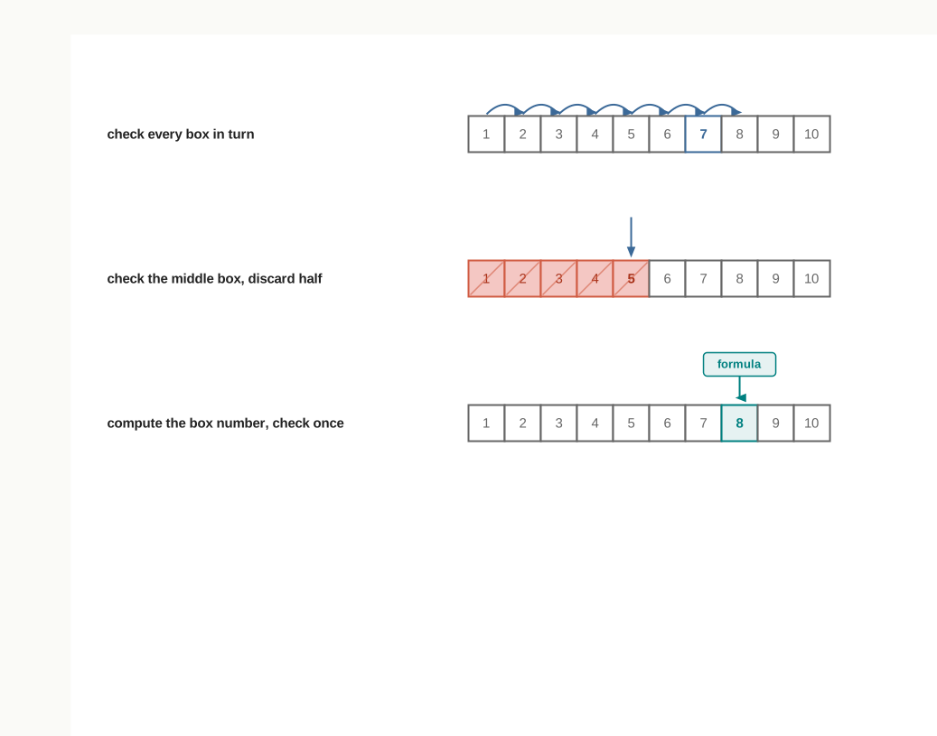
Fig. 6.0 – Three approaches to searching a collection.
The four sections that follow answer each of these questions in turn.
6.1 Introduction
A school library keeps a few thousand books. When you ask for one by name, the librarian does not walk along every shelf reading every spine. The books are arranged by subject and then by author, and that arrangement is what makes the request answerable in half a minute rather than half an afternoon. Now think of the same library with its books piled in no order at all. The book is still there, and it can still be found — but only by looking at one book after another until it turns up.
Both situations occur inside a computer, constantly. A program stores data so that it can be brought back later, and bringing it back means locating it first. Every time a result is looked up by roll number, a word is checked against a spell-list, or a bank record is fetched by account number, some collection is being examined for one particular item.
The interesting question is not whether the item can be found. Given enough time, any collection can be examined completely. The question is how much work the finding costs, and what property of the collection can be exploited to make that work smaller.
6.1.1 What It Means to Search a Collection
Searching means locating a particular element in a collection of elements. The result of a search tells you first whether that element is present in the collection at all, and if it is present, where it is.
The element you are looking for is called the key. The key is not part of the collection; it is the value you carry to the collection and hold up against the elements there. In a list of marks the key might be 72; in a list of words the key might be "Amazing".
Two possible outcomes
A search that finds the key is called a successful search, and it can report the position at which the key was found. A search that examines all the possibilities and does not find the key is an unsuccessful search, and it reports only that the key is absent.
Both outcomes are useful answers. A program that checks whether a roll number has already been entered wants the search to fail — an unsuccessful search is exactly the confirmation it needs before adding the record.
The collection in this chapter is a Python list, and a list keeps its elements in fixed positions. You met this in Class XI: the first element of a list sits at index 0, the second at index 1, and the last at index len(numbers) - 1. Any element can be reached directly by its index, without stepping through the ones before it.
That last property is worth pausing on, because the whole chapter rests on it. Reaching numbers[6] costs a computer no more than reaching numbers[0]. If a list could only be read from the front, the way a cassette tape had to be wound through, binary search would not be possible at all.
We refer to the figure below throughout the rest of this section. Fig. 6.1 shows a list, a key held beside it, and the two ways a search can end.
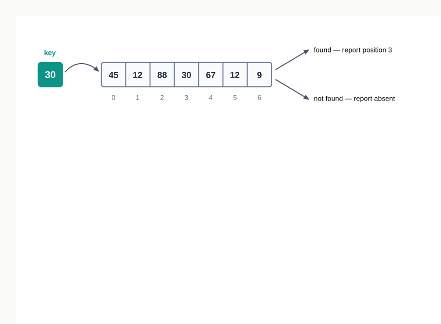
Fig. 6.1 – A list, a search key, and two possible outcomes.
Position or index?
Fig. 6.1 raises a small trap. The value 30 sits at index 3, but a person counting the boxes aloud would call it the fourth item. Both statements are correct; they use different conventions.
Python indexes from 0, while people count from 1. A search program must therefore decide which of the two it reports, and say so plainly. If a program returns the position as index + 1, then position 1 means the first element, and a returned value of 0 cannot mean anything at all.
Notice too that 12 appears twice in Fig. 6.1, at index 1 and at index 5. A collection may hold duplicate values, and a search that stops at the first match will never report the second. That is a design decision, not an error, but it must be a decision you have made knowingly.
6.1.2 Measuring the Work a Search Does
To say that one search method is better than another, we need a way of measuring the work each does. Timing them with a stopwatch is the obvious idea, and the wrong one. The same program timed on a newer machine, or on a machine running fewer other tasks, gives a different answer, and the comparison tells you about the machines rather than about the methods.
So we count instead of timing. In searching, almost all the work is one repeated action: taking the key and testing it against an element of the collection. That single test is called a key comparison.
Counting comparisons is machine-independent. A method that needs 500 comparisons where another needs 9 will be slower on every computer, and will still be slower next year.
The same method, different amounts of work
Here is the point that makes the measurement interesting. Run the same search method on the same collection twice, with two different keys, and the count changes. Looking for the element that happens to sit at the front is quick; looking for the one at the far end is not.
A single number therefore cannot describe a method. We describe it by its extremes instead. The best case is the arrangement of key and collection that makes the method do the least work. The worst case is the arrangement that makes it do the most.
Of the two, the worst case matters more. It is the promise a method can actually keep. Knowing that a search “is usually fast” is of little use when designing a system that must respond in time on every request, including the awkward ones.
For each of the three methods in this chapter, then, we shall ask the same four questions: what does the method require of the collection, how does it work, how many key comparisons does it make in the best and worst cases, and where does it fail. Table 6.1 previews the answers to the first of those questions.
Read the middle column carefully, because it carries the argument of the whole chapter. The methods get faster as you go down the table, but they also demand more of the collection before they will work. Speed here is not free; it is bought with preparation done earlier.
6.2 Linear Search
Suppose a games teacher is holding a bundle of eight score slips from a house match, in the order the students handed them in. She wants to know whether anyone scored exactly 12. There is nothing clever she can do. She has to look at the first slip, then the second, and keep going until she either finds a 12 or reaches the bottom of the bundle.
That is the whole of linear search. It is the method you fall back on when the collection offers you no help at all.
6.2.1 The Method of Linear Search
Linear search compares the key with every element of the collection, one after another, beginning at the first element and moving towards the last. If an element matches the key, the search stops there and reports success. If the end of the collection is reached with no match, the search reports that the key is absent.
Because the elements are examined in sequence, this method is also called sequential search or serial search. The three names describe the same method.
Two features of linear search follow from that definition and are worth naming at once.
It makes no demand on the collection. The elements may be sorted, reverse sorted or in complete disorder; the method behaves the same way. Nothing needs to be prepared before the search begins.
It is exhaustive. To declare a key absent, linear search must have compared it with every element, because any element it skipped might have been the one.
A list to work with
Table 6.2 shows the eight scores in the order they were collected, with the index of each.
Searching for the key 12 in this list means asking eight questions in the worst case, and stopping early if one of them is answered yes. Fig. 6.2 shows the first few of those questions.
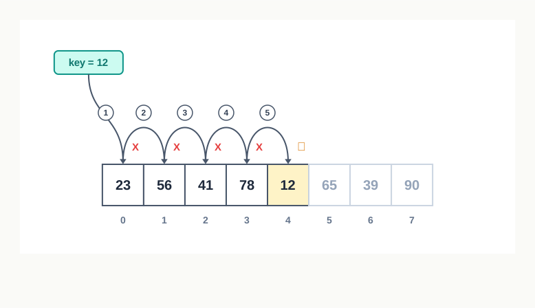
Fig. 6.2 – Linear search for the key 12.
Notice in Fig. 6.2 that the last three boxes are never looked at. The search stopped as soon as it succeeded, which is the only saving linear search ever makes.
6.2.2 The Linear Search Algorithm
Before writing any code, state the method as a sequence of steps. Two things have to be got right: the position must move forward by exactly one each time, and the “not found” answer must be given only after the last element has been tested.
6.2.3 Linear Search in Python
The algorithm translates into Python almost line for line. A for loop over range(len(numbers)) supplies the indices 0 to n-1 in order, so the counter of step 4 is managed for us.
Writing the search as a function keeps it reusable and keeps the searching separate from the printing. The function returns a value; deciding what to display with that value is the caller’s business.
6.2.4 Best Case, Worst Case and an Unsuccessful Search
Run the same program with different keys and the number of key comparisons changes, although nothing about the list or the method has changed. Table 6.4 records what happens for five different keys on the list of Table 6.2.
Read the first and last rows together. The best case for linear search is a key sitting at the very front: one comparison, whatever the length of the list. A list of a hundred elements and a list of a lakh of elements both answer in a single step if the key happens to be first.
The worst case is two situations that cost the same. A key sitting at the last position is found only after all \(n\) elements have been tested. A key that is absent altogether is also reported only after all \(n\) elements have been tested. Both take exactly \(n\) key comparisons, where \(n\) is the number of elements in the list.
Why absence costs the most
The absent key is the case worth thinking about hardest, because it exposes what the method does and does not know as it goes.
After comparing the key with scores[0] and failing, the search has learnt one fact: the key is not at index 0. It has learnt nothing whatsoever about indices 1 to 7. The elements are in no order, so a failure at one position says nothing about the positions ahead. Every comparison discards exactly one candidate and leaves the rest untouched.
To conclude that a key is absent, all \(n\) candidates must be discarded, and that requires all \(n\) comparisons. Stopping earlier would mean declaring an answer about elements never looked at.
This also explains something practical. If a program searches the same unsorted list again and again, the failures are as expensive as the successes, and they are what will dominate the running time in an application such as checking whether an entry is new.
6.2.5 Where Linear Search Is the Right Choice
It is tempting to treat linear search as merely the slow method, to be abandoned as soon as a faster one is learnt. That is not right, and the reason it is not right is worth understanding.
Linear search asks nothing of the data. That freedom is its advantage. It works on a list straight from the user, on records read from a file in the order they were written, and on a collection being added to while the program runs. Every faster method in this chapter first requires the collection to be put into a particular condition, and putting it into that condition costs work.
So linear search is the sensible choice when the collection is small, when its elements are in no order and are not worth ordering, or when the search will be done only once or twice. Sorting a list of twenty entries to search it a single time spends more effort on the preparation than the search could ever save.
Its honest limitation is equally clear. The work grows in direct proportion to the size of the collection. Doubling the number of elements doubles the worst-case cost. A method that needs ten comparisons on ten elements needs ten lakh on ten lakh elements, and no amount of careful coding changes that — the growth is in the method, not in the program.
That limitation is what the next section sets out to remove, by demanding something of the collection in return.
6.3 Binary Search
A class teacher holding a mark sheet of sixty students, arranged by roll number, is asked for the marks of roll number 47. She does not begin at roll number 1. She opens the sheet somewhere near the lower half, sees roll number 41, and knows instantly that 47 lies below that line — every entry above it can be ignored.
She has done something linear search can never do. From a single glance she has eliminated forty entries at once, without reading any of them. What made this possible was not cleverness but arrangement: the sheet is in order, and order lets one comparison speak about many elements.
6.3.1 Why Order Makes Searching Faster
Recall what a failed comparison achieves in linear search. Comparing the key with one element of an unordered list and finding no match rules out that element and nothing else. Each comparison buys you exactly one discarded candidate, which is why \(n\) elements cost \(n\) comparisons.
Now put the same elements in increasing order and compare the key with the element in the middle. Suppose the key is smaller. Every element after the middle is at least as large as the middle element, so every one of them is larger than the key too. The entire second half is eliminated by that one comparison.
This is the whole gain, and it is worth stating plainly: in an ordered collection, a comparison that fails still tells you which side the key must be on. The failure is informative. In an unordered collection it is not.
A sorted list is a list whose elements are arranged in order of their values — increasing or decreasing for numbers, alphabetical for text. Everything in this section assumes the list is sorted in increasing order, which is the usual arrangement.
6.3.2 The Method of Binary Search
Binary search compares the key with the element in the middle of a sorted list. Exactly one of three things happens.
If the middle element equals the key, the search succeeds and ends there.
If the middle element is greater than the key, then the key — if it is present at all — must lie before the middle. The second half, including the middle element itself, is discarded and the search continues in the first half.
If the middle element is less than the key, the key must lie after the middle. The first half, including the middle element, is discarded and the search continues in the second half.
The search area and its three markers
To carry this out, the method has to keep track of the part of the list still under consideration. That part is called the search area, and three index values describe it: first, the index of its leftmost element; last, the index of its rightmost element; and mid, the index of the element halfway between them, computed as (first + last) // 2.
At the start, first is 0 and last is n - 1, so the search area is the whole list. Table 6.5 shows a sorted list of eleven bus fares, and Fig. 6.3 marks these three positions on it.
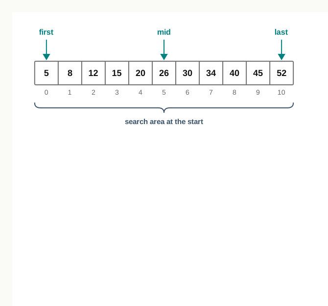
Fig. 6.3 – Initial search area and markers for binary search.
Notice in Fig. 6.3 that mid is (0 + 10) // 2, which is 5, so the middle element is 26. With eleven elements the middle is exact — five elements lie on either side of it.
When the number of elements is even there is no exact middle, and floor division settles the matter. For a search area running from index 0 to index 9, mid is (0 + 9) // 2, that is 4. The two halves then have four and five elements. The method does not require the halves to be equal; it only requires that each step throws one of them away.
How the search area shrinks
After the comparison at mid, the discarded half is dropped by moving one marker. If the key is smaller than the middle element, the new search area ends just before the middle, so last becomes mid - 1. If the key is larger, the new search area begins just after the middle, so first becomes mid + 1.
The - 1 and the + 1 are not decoration. The middle element has already been compared and does not match, so it belongs in neither half. Leaving it in — writing last = mid instead of last = mid - 1 — means a search area that stops shrinking once it reaches one element, and the method never terminates.
Eventually one of two things happens. Either an element at mid matches the key, or the search area shrinks away to nothing. It is empty when first becomes greater than last, and at that moment the key is known to be absent.
We use the word iteration rather than comparison for one pass of binary search, because a pass does more than compare: it also redefines the search area by moving first or last before the next comparison is made.
6.3.3 The Binary Search Algorithm
Written out as steps, the method looks like this. Read step 3 carefully — mid is recomputed at the start of every pass, from the current first and last. Computing it once before the loop is the single most common way of getting this algorithm wrong.
6.3.4 Binary Search in Python
The algorithm becomes a while loop with three branches inside it. As before, the search is written as a function that returns an index or None.
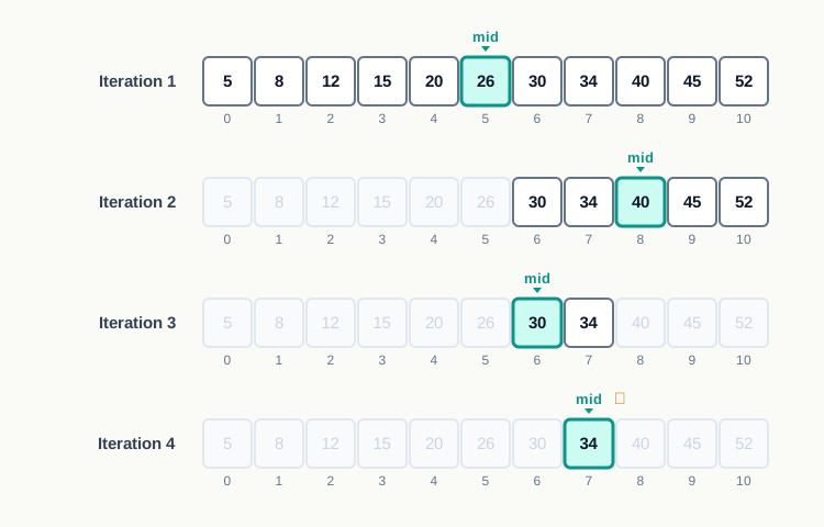
Fig. 6.4 – Binary search iterations for the key 34.
Fig. 6.4 makes the important point visible. The list is untouched throughout. What changes from row to row is only which part of it is still worth looking at.
When the key is absent
The same function, given a key that is not in the list, ends when the markers cross. Trace it for the fare 25, which no bus on this route charges.
That is a sharp difference from the previous section, where an absent key was the most expensive case of all.
6.3.5 Best Case and Worst Case
The best case for binary search is a key sitting exactly at the middle of the list. It is found in the first iteration, with one key comparison, whatever the size of the list. This is the least work binary search can do to confirm that a key is present.
The worst case is a key that forces the search area to be halved until only one element is left — or that is absent, so the halving continues until the search area is empty. Both cost the same, as the two dry runs above showed.
To count that worst case, ask how many times a collection of \(n\) elements can be halved before nothing is left. Eleven elements become five, then two, then one, then none: four steps. A hundred elements become fifty, twenty-five, twelve, six, three, one, none: seven steps. The number of halvings needed for \(n\) elements is \(\lfloor \log_2 n \rfloor + 1\), where \(\log_2 n\) is the power to which 2 must be raised to give \(n\), and \(\lfloor\ \rfloor\) means the whole-number part.
Table 6.7 puts that formula beside the count for linear search.
Read down the two columns and the difference is not one of degree. Multiplying the list size by ten multiplies the linear search count by ten, but adds only about three to the binary search count. Going from a thousand elements to ten lakh — a thousandfold increase — takes binary search from ten iterations to twenty.
The trade is now explicit. Binary search is dramatically faster, but it will only work on a sorted list, and keeping a list sorted has its own cost whenever new elements are added.
6.3.6 Applications of Binary Search
Binary search appears wherever data is kept in order and looked up repeatedly.
A dictionary, a telephone directory and a library catalogue are all sorted collections, and looking something up in any of them is binary search performed by hand. You open near the middle, decide which way to go, and repeat.
Inside a database, an index is a sorted structure built over a column precisely so that a lookup does not have to read every record. Searching that index uses the halving idea, extended to work on data held on disk rather than in memory.
A router keeps a table of destinations that must be consulted for every packet it forwards, and keeping that table ordered allows the lookup to be done by repeated halving rather than by scanning.
The idea also solves problems that are not obviously searches. If a fault first appeared somewhere in a long, ordered sequence of software revisions, testing the middle revision tells you which half contains the first bad one, and about twenty tests are enough to pinpoint it among ten lakh revisions. Finding the position at which a new value should be inserted into an already sorted list is the same method too — the search runs until the markers cross, and the crossing point is exactly where the new value belongs.
6.3.7 Linear Search and Binary Search Compared
The two methods answer the same question and are not otherwise alike. The distinction that matters is not which is faster, but what each demands before it can be used.
The last two rows carry the practical advice. For a list of twenty entries searched once, sorting first is wasted effort and linear search is the right answer. For a list of a lakh of entries searched all day, the sorting pays for itself many times over.
There is one situation where linear search wins outright regardless of size: when the collection changes constantly. Every insertion into a sorted list must be placed correctly, and if the data arrives faster than it is searched, the effort of maintaining order exceeds anything binary search returns.
6.4 Search by Hashing
Both methods so far have one thing in common: they look. Linear search looks at every element, binary search looks at fewer and fewer, but each of them examines elements until it can decide.
Now think about how a cloakroom at a railway station works. You hand over a bag and receive a token numbered 47. When you come back, nobody searches through the racks. The attendant walks straight to slot 47, because the number on the token is the location. The bag was not put down wherever there was room; it was put down where its number said it should go.
That is the idea this section develops. If an element’s value decides where it is stored, then finding it later needs no searching at all — only a calculation.
6.4.1 The Idea Behind Hashing
Hashing is a technique in which the position of an element in a table is computed from the element’s own value, using a fixed formula. To look for a key, the same formula is applied to the key, and only the one position it names is examined.
Read that last sentence again, because it is doing something the earlier methods could not. The search does not narrow down a region and then examine it. It calculates a single index and checks that index. The size of the collection never enters the calculation.
Because exactly one position is examined, a hash-based search makes exactly one key comparison — and it makes that one comparison whether the table holds ten elements or ten lakh.
6.4.2 Hash Function and Hash Table
Two things are needed: the formula, and the table it fills.
The formula is called a hash function. It takes an element and produces an integer index. That index is called the hash value of the element.
The table filled by the hash function is called a hash table. It is an ordinary list, with positions indexed from 0, in which each position holds either one element or nothing at all. Positions that hold nothing are marked None.
Note two things about the table’s size. It is fixed before any element is stored, because the hash function needs it. And it may be larger than the number of elements to be stored — usually it is, because a table packed to the last position leaves the hash function no room to place anything without a clash.
The remainder method
The simplest hash function for whole numbers is the remainder method. It divides the element by the size of the hash table and takes the remainder:
\[h(\text{element}) = \text{element} \bmod \text{size of the hash table}\]
In Python the remainder operator is %, so this is written element % size. The remainder on dividing by 10 is always one of \(0, 1, 2, \ldots, 9\), so a table of size 10 is exactly the right length — every hash value it can produce is a valid index, and no index is unreachable.
That is the property the method relies on. Taking the remainder by the table size guarantees an index inside the table, whatever the element’s value. The number 45 and the number 4,50,005 both land somewhere in the ten slots.
Consider seven book codes recorded by a school library, in the order the books were catalogued:
45, 61, 23, 88, 17, 39, 74
Applying element % 10 to each gives the hash values in Table 6.9.
For this particular set of codes the last digit of each is different, so the seven hash values are all different and each element gets a position of its own. Table 6.10 shows the table after all seven have been placed.
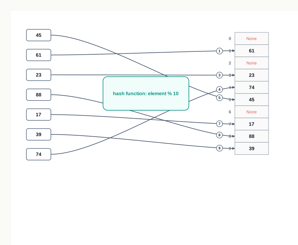
Fig. 6.5 – Storing elements in a hash table using the remainder method.
Notice in Fig. 6.5 that the original order is completely lost. In Table 6.10, 74 sits before 45 although it came later in the catalogue, and three slots are empty. A hash table is not a rearrangement of the list; it is a different structure built from it.
6.4.3 Building and Searching a Hash Table
The table is built first, once, and searched afterwards, as often as needed.
To build it, start with a list of the chosen size filled with None, then take each element in turn, compute its hash value, and store it at that index.
To search it, compute the hash value of the key and look at that one index. If the element stored there equals the key, the key is present. If not — whether the slot holds None or holds some other value — the key is absent, because if it had been stored at all it would have been stored precisely there.
Three ways a search can end
Run hash_find with three different keys on this table and three different things happen, all of them in one comparison.
For the key 39, the computed index is 9 and slot 9 holds 39. The key is present.
For the key 50, the computed index is 0 and slot 0 holds None. The key is absent, and the empty slot proves it — had 50 ever been stored, it would have been stored at index 0.
For the key 27, the computed index is 7 and slot 7 holds 17. The key is absent again, and this case is the interesting one. Two different values can share a hash value; 17 and 27 both end in 7. Finding a different element in the slot does not mean the key is elsewhere, it means the key was never stored — because if it had been, it would have been in that very slot.
6.4.4 Collision and Collision Resolution
Everything above rested on a quiet assumption: that the seven codes produced seven different hash values. Nothing guarantees that.
Suppose the library catalogues one more book with the code 35. Its hash value is 35 % 10, which is 5 — and slot 5 already holds 45. Both values end in the digit 5, and the remainder method sees only that digit.
When two elements have the same hash value, they are directed to the same position in the hash table. This situation is called a collision.
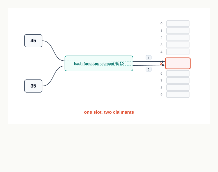
Fig. 6.6 – A collision in a hash table.
A collision is a genuine problem, not a nuisance to be waved away. A position in the hash table can hold exactly one element. In the program of the previous subsection the line hash_table[item % size] = item would simply overwrite 45 with 35, and 45 would vanish from the table without any warning. A later search for 45 would look in slot 5, find 35, and report the book as absent although it is on the shelf.
So a hash table needs a rule that says where to put the second and later elements that claim an occupied slot. The process of finding such a place is called collision resolution.
Several methods of collision resolution exist. Their details lie beyond this course; what matters here is that no hash table is usable in practice without one, and that every one of them costs something — the search may then have to examine more than a single position, and hashing loses a little of the guarantee that made it attractive.
6.4.5 Perfect Hash Functions and the Cost of Hashing
A hash function that maps every element of a given collection to a distinct index is called a perfect hash function. If a hash function is perfect for the data it is used on, collisions never occur and every search really does take one comparison.
The word “perfect” is easily misread. It does not describe a formula that is good in general; it describes a formula that happens to fit one particular set of elements. The remainder method with size 10 was perfect for the seven codes of Table 6.9, and stopped being perfect the moment the code 35 arrived. Perfection is a relation between a function and the data it is given, and new data can destroy it.
Besides the remainder method, hash functions can be built in other ways — by folding a long number into parts and adding them, by squaring the element and taking the middle digits, and by several other techniques. All of them aim at the same target: spreading the elements as evenly as possible over the available slots.
What hashing costs
The time a hash function takes does not depend on how many elements are stored. Computing 45 % 10 costs the same whether the table holds seven elements or seven thousand. That constancy is the whole advantage of hashing, and it is what neither linear nor binary search can offer.
But the calculation must be cheap. A hash function so elaborate that computing it takes longer than a handful of comparisons would defeat the purpose entirely — you would have replaced a short search with a long sum.
Hashing has three further costs that must be stated honestly. It uses memory for slots that stay empty; Table 6.10 reserved ten positions to hold seven elements. It loses the order of the data completely, so a hash table cannot be read out in increasing order, and it cannot answer a question such as “which codes lie between 20 and 50” — for that, binary search on a sorted list is the right tool. And it needs a collision resolution rule before it can be trusted with real data.
Read the first and last rows together, and the chapter’s argument closes where it began. Each method buys its speed by demanding something of the data beforehand — nothing, order, or a computed arrangement — and each pays for that speed in a different currency.
6.5 Summary
Searching means locating a particular element, called the key, in a collection of elements. The result of a search says whether the key is present, and if it is present, at what position.
A search that finds the key is a successful search; one that examines all the possibilities without finding it is an unsuccessful search. Both are useful answers, and an absent key is often exactly what a program needs to confirm.
Python indexes a list from 0, while people count positions from 1. A search must state which of the two it reports, and its failure value must be something that could never be mistaken for a valid index.
The work a search method does is measured by counting key comparisons, not by timing the program. A count is independent of the machine, so it compares the methods rather than the computers they run on.
The same method does different amounts of work on different keys, so it is described by its extremes. The best case is the situation needing the fewest key comparisons, the worst case the situation needing the most; the worst case matters more, because it is the promise the method can keep.
This chapter covers three methods: linear search, binary search and search by hashing. Each is faster than the one before it, and each demands more of the collection before it will work at all.
Linear search compares the key with each element in turn, from the first towards the last, stopping at a match. Because the elements are examined in sequence, it is also called sequential search or serial search.
Linear search makes no demand on the arrangement of the collection, which is its real advantage. It works on sorted data, reverse-sorted data and data in complete disorder, with no preparation.
In an unordered collection a failed comparison rules out only the one element it tested, and says nothing about the elements not yet examined. This is why an unsuccessful linear search must compare the key with every element before it can report absence.
For a list of \(n\) elements, linear search needs 1 key comparison in the best case, when the key is the first element, and \(n\) key comparisons in the worst case, when the key is the last element or is absent. Doubling the size of the list doubles the worst-case work.
Binary search requires the list to be sorted. It compares the key with the middle element of the current search area, and one of three things follows: the middle element equals the key and the search ends, or it is greater than the key and the second half is discarded, or it is less than the key and the first half is discarded.
Order is what makes this discarding legitimate. In a sorted list, a comparison that fails also reveals which side of the middle the key must lie on, so a single failed comparison eliminates an entire half.
The search area is described by three indices: the first element, the last element, and the middle computed by floor division of their sum by two. The middle must be recomputed at the start of every pass, because the middle of a search area is meaningless once the search area has moved.
The discarded middle element is excluded from the half that remains, so the marker moves to one position beyond it. Leaving the middle element inside the surviving half stops the search area from shrinking, and the method then never ends.
Binary search ends either at a match or when the two markers cross, which means the search area has become empty and the key is absent. It never changes the list; only the indices of the search area change.
For a list of \(n\) elements, binary search needs 1 key comparison in the best case, when the key is the middle element, and about \(\lfloor \log_2 n \rfloor + 1\) iterations in the worst case. An unsuccessful binary search costs the same as the worst successful one, which is a sharp contrast with linear search.
Because the growth is by halving, multiplying the size of the list by a thousand adds only about ten iterations. Ten lakh sorted elements can be searched in about twenty iterations.
Used on an unsorted list, binary search does not fail loudly. It runs, ends and may report a present element as absent, because a discard is only justified when order guarantees that the discarded half cannot hold the key.
Binary search is worth its preparation when a collection is large and searched often; sorting a small collection to search it once costs more than it saves. Where data changes constantly, maintaining the order can outweigh the benefit altogether.
Hashing computes the position of an element from the element’s own value, using a formula called the hash function; the index it produces is the hash value, and the list that holds the elements at those indices is the hash table.
Each position of a hash table holds at most one element, and unused positions hold the value none. The table size is fixed before storing begins, and is usually larger than the number of elements to be stored.
The remainder method is the simplest hash function for whole numbers: the hash value of an element is the remainder left on dividing it by the size of the hash table. Taking the remainder by the table size guarantees an index that lies inside the table.
Searching applies the same hash function to the key and examines only the computed position. If that position holds the key, the key is present; if it holds anything else, including nothing at all, the key is absent, because it could only ever have been stored there.
A hash-based search therefore takes one key comparison, and takes it regardless of how many elements the table holds. The time to compute a hash value does not depend on the size of the collection, which is what neither linear nor binary search can offer.
The storing rule and the searching rule must use the same hash function and the same table size. If they differ, the search looks in a slot the element was never placed in, and reports a wrong answer without raising any error.
A collision occurs when the hash function gives the same hash value to two or more different elements, directing them to the same position. Since a position can hold only one element, an unguarded collision silently overwrites the element already there.
Collision resolution is the process of deciding where to store an element whose position is already occupied. Every method of resolving collisions costs something, and once collisions occur, the promise of a single key comparison weakens.
A perfect hash function gives a different hash value to every element of a given collection, so no collision can occur. Perfection is a relation between a formula and one particular set of data, and new data can destroy it.
Hashing is paid for in memory, in lost order and in the need for a collision rule. A hash table reserves slots that stay empty, cannot be read out in order of value, and cannot answer questions about a range of values — for those, a sorted list and binary search remain the right tools.
6.6 Key Terms
Best case — the situation in which a search method performs the fewest key comparisons for a collection of a given size.
Binary search — a search method for a sorted list that compares the key with the middle element of the current search area and discards the half that cannot contain the key.
Collision — the situation in which a hash function gives the same hash value to two or more different elements, directing them to the same position in the hash table.
Collision resolution — the process of deciding where to store an element whose hash value names a position that is already occupied.
Hash function — a formula that takes an element and produces an integer index at which that element is to be stored.
Hash table — a list in which each element is stored at the position given by its hash value, each position holding at most one element.
Hash value — the integer index produced for an element by the hash function.
Hashing — a searching technique in which an element’s storage position is computed from the element itself, so that a key can be located by calculation rather than by examining elements one after another.
Iteration — one complete pass of binary search, in which the middle element is compared with the key and the search area is then redefined.
Key — the value being searched for, supplied to the search and compared against the elements of the collection.
Key comparison — one test of the key against one element of the collection, used as the unit for measuring the work a search method does.
Linear search — a search method that compares the key with the elements of a collection one by one, in the order in which they occur, until a match is found or the collection is exhausted.
Perfect hash function — a hash function that gives a different hash value to every element of a given collection, so that no collision can occur.
Remainder method — a simple hash function for whole numbers, in which the hash value of an element is the remainder left on dividing it by the size of the hash table.
Searching — the process of locating a given element in a collection, so as to determine whether it is present and, if so, at what position.
Sequential search — another name for linear search, describing the fact that the elements are examined in sequence.
Serial search — another name for linear search.
Sorted list — a list whose elements are arranged in order of their values, increasing or decreasing for numbers and alphabetical for text.
Successful search — a search that finds the key in the collection and can report its position.
Unsuccessful search — a search that examines all the possibilities and reports that the key is not present in the collection.
Worst case — the situation in which a search method performs the most key comparisons for a collection of a given size.
6.7 Points to Ponder
Linear search demands nothing of the collection, and that is exactly why it is the slowest method here. Is “requires no preparation” a weakness or a strength, and what would you need to know about an application before deciding which it is?
Binary search throws away half a list on the evidence of one comparison. What precisely does sortedness guarantee that makes so large a conclusion safe from so small a piece of evidence — and what is the smallest change to the list that would destroy that guarantee?
A hash table answers “is it there?” in one comparison but cannot list its contents in order, or say which values lie between 20 and 50. If a structure is faster at one question and incapable of another, is “faster” still the right word to compare the two?
The idea of binary search can be explained in a sentence, yet correct programs for it took years to appear in print. Why are the boundary cases of an algorithm so much harder than its central idea, and how would you convince someone your search is correct without running it?
Sorting a list to search it once is wasteful; sorting it to search it a thousand times is essential. How would you work out, for a particular collection, the number of searches at which the sorting begins to pay for itself?
A hash function is called perfect only in relation to the data it is actually given, and new data can end that perfection. Can any storage arrangement be designed to be perfect for data that has not yet arrived, or is every such design a bet on what is coming?
6.8 Objective Questions
Which of the following is another name for linear search? [1 mark]
- Binary search
- Sequential search
- Hash search
- Ordered search
A sorted list contains 15 elements. The maximum number of iterations binary search can need on it is [1 mark]
- 3
- 4
- 8
- 15
During binary search, the element at the middle position is found to be greater than the key. The next step is to set [1 mark]
first = mid + 1last = mid - 1first = midlast = mid
A hash table has 13 positions and the hash function is
element % 13. The element 96 will be stored at index [1 mark]- 5
- 6
- 7
- 9
Fill in the blank: an unsuccessful linear search on a list of \(n\) elements makes ______ key comparisons. [1 mark]
State whether the following is true or false: on the same sorted list, an unsuccessful binary search needs fewer iterations than the worst successful one. [1 mark]
Match each item in Column A with the correct description in Column B. [1 mark]
| Column A | Column B |
|---|---|
| a. Linear search | i. Two different elements are directed to the same position |
| b. Binary search | ii. The position of an element is computed from its own value |
| c. Hashing | iii. Makes no demand on the arrangement of the elements |
| d. Collision | iv. Requires the elements to be in order of value |
- Assertion (A): A hash table is usually created with more positions than the number of elements to be stored. [1 mark] Reason (R): Increasing the size of a hash table makes collisions impossible.
- Both A and R are true, and R is the correct explanation of A.
- Both A and R are true, but R is not the correct explanation of A.
- A is true but R is false.
- A is false but R is true.
- Assertion (A): In linear search on an unordered list, finding the last element and failing to find the key cost the same number of key comparisons. [1 mark] Reason (R): In an unordered list, a comparison that fails rules out only the single element it tested.
- Both A and R are true, and R is the correct explanation of A.
- Both A and R are true, but R is not the correct explanation of A.
- A is true but R is false.
- A is false but R is true.
- Write the output of the following fragment. [1 mark]
data = [4, 11, 19, 26, 33]
print((0 + len(data) - 1) // 2)
6.9 Check Your Concepts
Define searching. State the two things the result of a search can tell you about the key. [2 marks]
What is a key comparison? Give one reason why the work of a search method is measured by counting key comparisons rather than by timing the program with a clock. [2 marks]
For a list of \(n\) elements, state the best case and the worst case of linear search, naming in each case where the key lies. [2 marks]
Differentiate between linear search and binary search on any three points. For each method, name one situation in which it would be the better choice. [3 marks]
Explain, using a short list of your own of at most six elements, how binary search can report a present element as absent when the list is not sorted. [3 marks]
What is a collision in hashing? Give one example using the hash function
element % 10, and explain why a collision cannot simply be ignored. [3 marks]Explain the working of binary search on a sorted list. Your answer should state which three index values describe the search area, how the middle is computed, how the search area changes after an unsuccessful comparison, and when the search stops. [4 marks]
A classmate says that hashing should always be preferred to binary search, because it settles a search in one key comparison. Give three reasons why this claim is not correct. [4 marks]
Write a Python function that takes a sorted list and a key and returns the index of the key by binary search, or
Noneif the key is absent. Then explain, in two or three sentences, why the middle position must be recomputed in every pass and why the marker moves one position beyond the middle rather than onto it. [5 marks]A collection of 20,000 records is to be searched. Work out the worst-case number of key comparisons for linear search and the worst-case number of iterations for binary search, showing your reasoning. State what preparation binary search requires, and describe one situation in which that preparation would not be worth doing on this collection. [5 marks]
6.10 Output & Debugging
- Study the fragment and answer both parts. [2 marks]
values = [7, 12, 19, 25, 31, 40]
key = 19
count = 0
for i in range(len(values)):
    count = count + 1
    if values[i] == key:
        break
print(count)
a. Write the output of the fragment.
b. State in one line what the variable `count` measures.- Study the program and answer both parts. [3 marks]
def search(numbers, key):
    first = 0
    last = len(numbers) - 1
    while first <= last:
        mid = (first + last) // 2
        if numbers[mid] == key:
            return mid
        elif numbers[mid] < key:
            first = mid + 1
        else:
            last = mid - 1
    return -1

marks = [12, 25, 33, 41, 56, 68, 79]
print(search(marks, 68), search(marks, 30))
a. Write the output of the program.
b. For the second call only, write the values of `first`, `last` and `mid` in each pass of the loop.- The following function contains one error. [3 marks]
def linear_search(numbers, key):
    index = 0
    while index < len(numbers):
        if numbers[index] == key:
            return index
    return None

print(linear_search([9, 14, 21], 21))
a. State what happens when this program is run.
b. Identify the error and rewrite the corrected function.- Study the fragment and answer both parts. [3 marks]
table = [None] * 7
for item in [15, 22, 9, 30]:
    table[item % 7] = item
print(table)
a. Write the output of the fragment.
b. Two of the four numbers do not appear in the printed table. Name them and explain why they are missing.6.11 Case-Based Questions
- A school library records the code of every book issued during the day, in the order in which the books were issued. At the end of one day the record is:
[318, 145, 902, 267, 145, 573, 88, 410]a. The librarian wants to know whether the book with code 573 was issued that day. Which of the three search methods of this chapter can be used on this record as it stands, and why can the other two not be used directly? [1 mark]
b. How many key comparisons will that method make to answer for the code 573, and how many for the code 200? Give a reason for the second figure. [2 marks]
c. The code 145 appears twice. State what a search function that returns at the first match will report, and describe one change that would make it report every position at which 145 occurs. [1 mark]- A bus depot maintains the length in kilometres of each of its routes, arranged in increasing order:
[6, 11, 17, 24, 30, 38, 45, 52, 60, 71, 85]a. Apply binary search to look for the key 45. Write the values of `first`, `last` and `mid` in each iteration, and state how many iterations are needed. [3 marks]
b. State the maximum number of iterations binary search can need on this list, and name one key for which that maximum actually occurs. [1 mark]
c. The depot decides instead to store these lengths in a hash table of 11 positions, using the hash function `length % 11`. State the index at which 45 would be stored, and give one question about the routes that the hash table cannot answer but the sorted list can. [1 mark]6.12 Programming Practice
Write a function
count_key(numbers, key)that uses linear search to return the number of timeskeyoccurs in the listnumbers. The function must examine every element and must not use any built-in counting method. Submit the function and one sample call with the output it produces, using a list that contains the key more than once. [3 marks]Write a complete program that reads 12 integers from the user into a list, arranges the list in increasing order, then reads a key and uses binary search to report the position of that key counting from 1, or a suitable message if the key is absent. The searching must be done by a function of your own, not by any built-in method. Submit the full program together with an identifier description table, and record the output for one key that is present and one that is not. [4 marks]
A sorted list must remain sorted when a new value is added to it. Write a function
find_place(numbers, value)that uses the binary search idea to return the index at whichvalueshould be inserted so that the list stays in increasing order. The function must not insert anything; it only returns the index. Submit the function, and the index it returns for the value 29 and for the value 90 when given the list[8, 15, 22, 34, 41, 57, 66]. [4 marks]A class has eight practice roll numbers, each of two digits, that are to be stored in a hash table of 13 positions using the hash function
roll % 13. Write a complete program that builds the table, but that prints a warning line naming both values whenever a roll number is directed to a position already occupied, instead of overwriting the entry silently. The program must then display the finished table and, for a roll number typed by the user, report whether it is present and at which index. Submit the full program, an identifier description table, and a note listing which of your eight values collided. [5 marks]