Chapter 7: Understanding Data
Once every ten years, India counts itself. Enumerators walk from house to house across cities, villages and hamlets, knocking on doors and filling in a schedule for each household — how many people live here, of what ages, who can read and write, what the house is built of, whether there is a source of drinking water nearby. The Census of India has been carried out in this decennial fashion since the nineteenth century, and it remains one of the largest peacetime data collection exercises anywhere in the world.
Now think about what the enumerator actually carries back. A stack of filled schedules is not, by itself, an answer to a single useful question. Nobody can read a few crore forms and announce how the country is changing. The forms have to be brought together, stored safely, arranged into rows and columns, and then reduced — averaged, counted, compared, ranked — until a page of a few numbers can stand in for millions of entries. Only at that point does a planner learn that one district needs more schools and another needs more water supply.
That gap between what is collected and what is finally understood is the subject of this chapter. Raw data are not information. Something has to happen in between, and that something is worth learning properly.
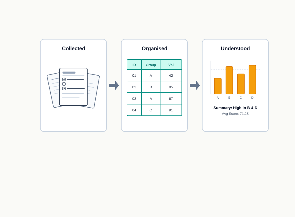
Fig. 7.0 – The transformation of data into information.
Keep these five questions in mind as you read. Each one is answered somewhere in this chapter, at the point where the idea behind it is explained.
7.1 Introduction to Data
Look at almost any decision that is made carefully rather than casually, and you will find something written down behind it. A student choosing a college looks at how many students were placed from it in earlier years, what the fees are, and how far the hostel is from the campus. A cricket coach preparing for a match studies how the opposing batters scored in their last few innings. A bank, before it releases money at a counter, checks what the account already holds. None of these people are guessing. Each of them is reading something that was recorded earlier.
Whatever is recorded in this way — the placement figures, the innings scores, the account balance — is data. Data are the raw facts and figures gathered from some situation, before anyone has interpreted them. A word of caution about the word itself: data is a plural form, and its singular is datum, so a careful writer says “the data are stored” rather than “the data is stored”. You will see both in everyday use, but the book keeps to the plural.
Data are not only numbers. A name is data, so is a date of birth, so is a photograph, an audio recording, a sensor reading and a comment typed under a video. The following are all things a computer is routinely asked to store as data:
- Personal particulars such as a name, an age, a class or a contact address
- Transaction records generated at a billing counter, a ticket window or an online payment
- Images, graphics, animations, audio and video
- Documents and web pages
- Posts, comments and messages on a social platform
- Signals produced continuously by sensors
- Satellite data, including meteorological readings and earth observation data
Data are not yet information
Here is the point on which the whole chapter turns. Suppose a college placement cell holds the records of every student placed over the last three years — the company, the role and the package for each one. That set of records, taken as it is, tells you almost nothing. You cannot read two thousand rows and form a judgement. What the brochure eventually prints is one line: the average package, the highest package, and the number of companies that visited. Those few numbers were not collected from anyone. They were produced from the collected records.
So data and information are not two words for the same thing. Information is what data become after they have been organised, summarised and interpreted for a purpose. Data are the input; information is the output.
Two further ideas run through this chapter and should be named now. Storing data in electronic form rather than in registers makes processing enormously faster, because a computer can sum, sort and count without tiring. And the information and communication technology (ICT) revolution — computers, mobile phones and the Internet together — has meant that data are now generated in far greater volume, and far faster, than any manual system was ever designed to handle.
7.1.1 Importance of Data
Human beings have always used data to decide. What is new is scale. When a large volume of data is processed by a computer, patterns emerge that no person could have noticed by reading the records one at a time — and it is those hidden patterns that make data valuable.
Consider some ordinary settings.
A bank must keep an accurate record of every account and update it the moment money is withdrawn at a counter or an automated teller machine (ATM); if the data were not maintained and updated, the very next withdrawal would be made against a wrong balance. A meteorological office watches satellite readings continuously, and it is the movement in those readings over hours — not any single reading — that produces a cyclone warning. A shop that records what each customer buys may discover that two unrelated items are very often bought together, and may then place them near each other so that both sell more.
The same reasoning explains why data are collected in settings that have nothing to do with business:
- Electronic voting machines record the votes cast, and the counts from all the machines are then accumulated, which is why a result that once took days of manual counting now takes hours.
- Scientists record readings during an experiment so that results can be compared across trials rather than trusted from memory.
- A hospital records patient details so that a later visit can be read against an earlier one.
- A library maintains data about its books and its members, so that it can tell at any moment which book is with whom.
- A search engine returns results by analysing an enormous volume of page data gathered from across the World Wide Web (WWW).
Notice what these have in common. In each case the value does not lie in any one record. It lies in the ability to compare, count and combine records — which is possible only because they were recorded in the first place, and recorded consistently.
7.1.2 Types of Data
Data arrive from many different sources, and they do not all have same shape. An image is a grid of pixels. A video is a sequence of frames. A fee slip is a handful of labelled entries, some numeric and some not. A chat message mixes text, icons and pictures. If you intend to process data with a computer, this difference in shape matters more than the difference in subject, because it decides what the computer can do with the data automatically.
On the basis of format, then, data fall into two broad categories: structured data and unstructured data. The contrast between the two is drawn in Fig. 7.1, and the sections that follow take each in turn.
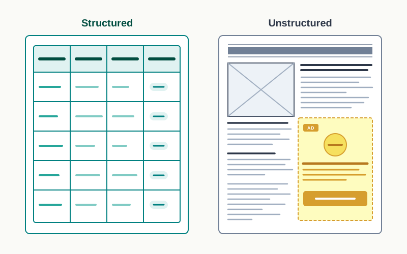
Fig. 7.1 – Structured and unstructured data.
7.1.2.1 Structured Data
Data that are organised and can be recorded in a well defined format are called structured data. In a computer, structured data are usually held in tabular form — in rows and columns. Each column holds one particular kind of fact, and that kind of fact is called an attribute (it is also called a characteristic or a variable). Each row holds the collection of attribute values belonging to one observation.
Table 7.1 shows structured data of the kind a school library keeps about the books it holds.
Read the table for a moment as the librarian would. The five entries in the CopiesAvailable column can simply be added, giving \(4 + 6 + 3 + 5 + 2 = 20\) copies on the shelves altogether. The total value of the stock needs a little more work: each price is multiplied by the number of copies of that title, and the five products are added, giving \(960 + 1080 + 960 + 750 + 520 = 4270\) rupees.
Neither calculation required anyone to understand what a book is. That is the whole point of structure. Because the price of every title sits in the same column, a spreadsheet or a program can be told “add this column” or “multiply this column by that one” and it will be right every time. The meaning has been built into the arrangement.
A second consequence of structure is that the attributes have to be decided before the data are collected. Table 7.2 lists some familiar activities together with the attributes that would have to be recorded for each.
Look down the middle row. If the person designing that booking system forgets to include TravelDate, then no amount of clever processing afterwards can recover it — the fact was never captured. Deciding the attributes is therefore a design decision, and a permanent one.
7.1.2.2 Unstructured Data
Now think about a newspaper. It is full of data — reports, photographs, notices, advertisements. But there is no fixed pattern to how they are placed. One day a page may carry three photographs of different sizes with five reports around them; the next day it may carry one large photograph and three reports. Nothing sits in the same place twice.
An email behaves the same way. There is no rule about how many paragraphs it contains, in what order the points appear, or how many files are attached. Data of this kind, which do not fall into the traditional row-and-column structure, are called unstructured data.
Web pages are unstructured, and so are text documents, business reports, books, audio and video files, and messages on social platforms. A photograph is unstructured data too: it is a large grid of pixel values, and there is no column in it labelled “who is in this picture”.
This does not mean unstructured data are useless or that nothing can be done with them — a great deal can, and specialised techniques exist for it. It does mean that the simple, reliable operations you saw on Table 7.1 are not available. You cannot ask a newspaper to add up its third column, because it does not have one. For this reason, the rest of this book works with structured data.
7.1.3 Metadata
Unstructured data are not left completely undescribed. Around almost every unstructured item there is a small amount of orderly, structured description attached to it, and this description is called metadata — which is simply data about data.
Take an email again. The message body has no fixed shape, but the subject line, the sender, the recipients, the date sent and the list of attachments certainly do. Those are the metadata of that email, and they are what let a mail program sort your inbox by date or search it by sender without ever reading a word of any message.
An image file works the same way, as Fig. 7.2 shows. The picture itself is a mass of pixel values, but stored alongside it are the file size in kilobytes or megabytes, the image type such as JPEG or PNG, and the resolution in pixels. These items are few, fixed and named — in other words, structured — and they are enough to let you arrange a folder of a thousand photographs by size or filter it by format.
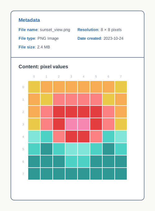
Fig. 7.2 – Unstructured data and its structured metadata.
7.2 Data Collection
Nothing can be processed that has not first been gathered. Before any of the techniques in this chapter can be applied, somebody has to decide what facts are needed, find or record them, and get them into a form a computer can read. That first step is called data collection.
It is worth being precise about what the step involves, because students often assume it always means going out and asking people. Frequently it does not. Much of the data an organisation needs has already been recorded by somebody, for some other purpose, and the real work is finding it and putting it into usable shape. Collection therefore covers two rather different activities: identifying data that already exist, and gathering fresh data from an appropriate source.
Start from the question, not from the data
The order matters here, and it is easy to get backwards. You do not begin by collecting whatever is available and then wonder what it might tell you. You begin with the question you intend to answer, work out which attributes that question depends on, and only then decide where those attributes will come from.
Suppose a school wants to know whether its morning bus routes are running to time. The question fixes the attributes at once: the route number, the scheduled arrival time, the actual arrival time, and the date. Nothing else needs recording. Had the question instead been about how crowded the buses are, the attributes would have been different — route number, date and number of passengers boarding. The same buses, the same mornings, but a different collection.
This is why the sequence in Fig. 7.3 is worth fixing in your mind. Each step in it is decided by the step before it, and a mistake at the front cannot be repaired at the back.

Fig. 7.3 – The data collection sequence.
Three situations you will actually meet
Take a neighbourhood stationery shop whose owner wants to know which items sell best in the weeks before a new school session. The sales data may be in one of three states, and each state calls for something different.
- The data exist, but only on paper. The owner has been writing every day’s sales in a register. The facts are all there, but a register cannot be sorted or totalled by a machine. Here the collection work is data entry — reading the register and typing its contents into a digital form, most simply a spreadsheet.
- The data already exist in digital form. Perhaps the billing counter software already writes out each day’s sales as a comma separated values (CSV) file — a plain text file in which the values of one record are written on one line, separated by commas. Here almost no collection work remains; the file is read as it stands.
- The data do not exist at all. Nothing has been recorded in either form, and the owner wants a system that will record sales from now on. Here collection has to be built into a piece of software, written in a language such as Python, which stores each sale as it happens — into a CSV file, or into a database, which is taken up in the next section.
Notice that the third situation is the only one in which you control the format from the start, and it is therefore the only one in which the data will be clean by design rather than by repair.
Modes of collecting fresh data
Where data must be gathered rather than found, the method has to suit what is being measured. Table 7.4 sets out the common modes.
The last row is quietly the most important one today. A toll plaza barrier records every vehicle that passes; a metro gate records every card that is tapped; an online learning platform records every lesson a student opens. Nobody is conducting a survey in any of these cases, yet enormous volumes of data are being generated all the time, simply as a by-product of the system doing its ordinary work. This is a large part of why the quantity of stored data has grown so steeply.
The data are only as good as the collection
A computer will process whatever it is given, and it will do so confidently. It has no way of telling that a temperature was written down as \(34\) when the instrument read \(43\). So the correctness of every result in the rest of this chapter rests entirely on the quality of the collection step, and four things are worth checking before the data go anywhere.
- Relevance — every attribute collected relates to the question being asked, and every attribute the question needs has been collected.
- Accuracy — the recorded value is the value that actually occurred, not a mistyped or mis-copied one.
- Completeness — records are not missing, and fields within a record are not left blank in a way that will later be mistaken for a zero.
- Consistency — the same fact is recorded the same way everywhere: one date format throughout, one spelling of each route name, one unit for every quantity.
The fourth is the one most often neglected, and it fails silently. If half the entries in a column read Delhi and the other half read New Delhi, a program counting entries by city will report two cities where there is one, and it will not warn you.
7.3 Data Storage
Once data have been gathered and processed, the obvious temptation is to keep the result and throw away the rest. Almost no organisation does this. The register of last year’s sales, the readings from last month’s experiment, the attendance of the term just finished — all of it is kept, because the questions that will be asked next year have not been asked yet, and only the original records can answer them.
Keeping data for that purpose is data storage: the process of holding data on a storage device so that they can be retrieved and used again later.
Memory and storage are not the same thing
Two words are used loosely in ordinary speech and must be kept apart here. When a program runs, the values it is working with are held in primary memory — the random access memory (RAM) of the machine. This memory is fast, and the processor reaches it directly, but it is volatile: switch the machine off and its contents are gone.
Secondary storage is different in every one of these respects. It is slower, the processor cannot work on it directly, and it is non-volatile — what is written there survives a power cut and a shutdown. Storage of this kind is described as persistent storage, meaning simply that the data persist after the program that created them has ended.
This is the whole reason a program that computes something must deliberately write it out. The calculation happened in memory; unless it was saved to storage, nothing of it remains the moment the program stops.
Devices on which data are stored
The cost of digital storage has fallen steadily over the years, which is fortunate, because the volume of data being generated has risen just as steadily. A great many storage devices are available, and Table 7.6 lists the commonly used ones.
Two things in that table are worth pausing on. A tape is read strictly from one end towards the other, so finding a single record on it means passing over everything before it — which is why tapes are excellent for backing up a whole year’s data and hopeless for answering one query. And the difference between an HDD and an SSD is not merely one of speed: a device with moving parts and a device with none fail in quite different ways, and are chosen for different jobs.
Measuring how much is stored
Storage capacity is measured in bytes. A bit is a single binary digit, \(0\) or \(1\); a byte is a group of \(8\) bits, historically enough to hold one character of ordinary text. Larger amounts are named in the usual way, where each step is a multiple of \(1024\):
\[1\ \text{KB} = 1024\ \text{bytes},\quad 1\ \text{MB} = 1024\ \text{KB},\quad 1\ \text{GB} = 1024\ \text{MB},\quad 1\ \text{TB} = 1024\ \text{GB}\]
Here KB stands for kilobyte, MB for megabyte, GB for gigabyte and TB for terabyte. You should be aware that storage device manufacturers often quote capacity in powers of ten instead, taking \(1\ \text{GB}\) to mean \(10^9\) bytes, which is why a drive sold as \(500\) GB is reported by the operating system as somewhat less. Neither figure is wrong; they are counting in different bases.
Files, and where files fall short
Data on a storage device are organised as files. Photographs, documents and audio recordings are stored as files, and so are the data of a school or an office. A program can add records to a file, modify them, delete them, or read the whole file to produce a result. This arrangement is called file processing, and for a single small task it works perfectly well.
It begins to fail as soon as several parts of an organisation keep their own files. Picture a school in which the office maintains one file of student details, the examination cell maintains its own file with the same names and classes plus marks, and the transport section maintains a third with the same names again plus bus routes. The arrangement is shown in Fig. 7.4.
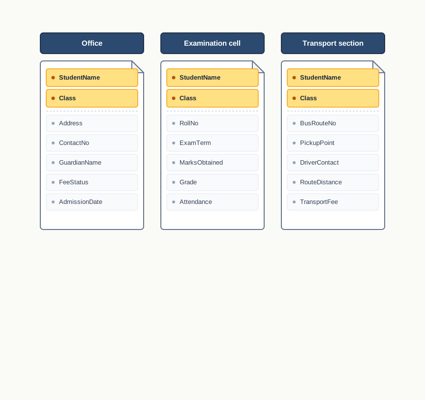
Fig. 7.4 – Data redundancy across separate files.
The same student’s name and class are now stored three times over. Storing the same fact repeatedly in this way is data redundancy, and it wastes space — which is the least of its problems. The real damage comes when a student changes section and only two of the three files are corrected. The files now disagree with one another, and there is no way to tell from the data which of them is right. Data that contradict themselves in this way are said to show data inconsistency.
File processing has other limitations of the same family. Each program has to know the exact layout of the file it reads, so a change in that layout means changing every program. Sharing the same file between several users working at once is difficult to manage safely. And a rule such as “no two students may have the same roll number” cannot be enforced by the file itself; it can only be enforced by every program that writes to it, which means it will eventually not be enforced at all.
These limitations can be overcome by a database management system (DBMS) — software that stores data centrally, controls how they are accessed, and enforces rules about what may be stored. That is a subject in its own right, and later chapters take it up properly. For now it is enough to see why it was needed: not because files are a bad idea, but because files scale badly once more than one program depends on them.
7.4 Data Processing
Data are collected because they hold facts worth knowing. But the facts are not visible in the raw records, and no amount of staring at a large file will make them appear. A term’s attendance register for a whole school runs to thousands of marks; the question “which class attended least regularly this term?” is answered by none of them individually and by all of them together. Something has to be done to the records to bring the answer out, and that something is data processing.
The shape of the whole activity is simple enough to state in one line, and Fig. 7.5 states it: raw data go in, processing happens, information comes out. The raw data may be numbers, text or images; the information that emerges is normally a table, a chart or a short piece of text that a person can actually read.
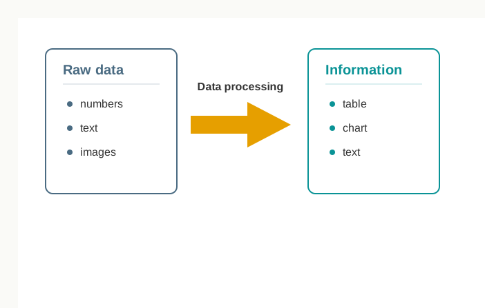
Fig. 7.5 – The data processing transformation.
7.4.1 The Data Processing Cycle
The middle arrow of Fig. 7.5 hides a good deal. Opened up, data processing has three stages — input, processing and output — and the whole arrangement is called the data processing cycle. Fig. 7.6 shows the stages with the activities that belong to each.
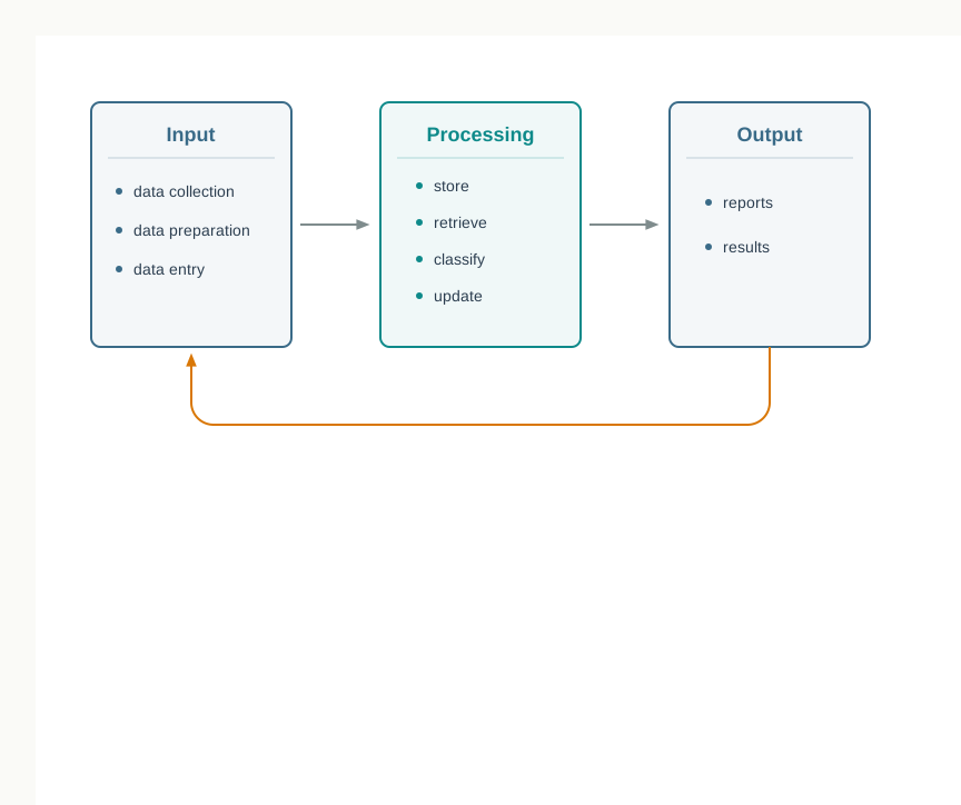
Fig. 7.6 – The data processing cycle.
Input
The input stage covers everything that has to happen before the machine can begin to compute. It has three parts.
The first is data collection, which section 7.2 has already dealt with. The second is data preparation, and it is the part most often skipped and most often regretted. Collected data are rarely fit to use as they arrive: a few records are duplicated, a few fields are blank, dates have been written in two different formats, a quantity has been entered in grams in one place and kilograms in another. Preparation means finding and fixing all of this before any calculation is run on it. The third part is data entry, in which the prepared data are actually put into the system — typed in, read from an existing file, or captured automatically by the equipment that generated them.
The reason preparation matters is worth stating plainly. A program cannot tell a wrong value from a right one; it will calculate an average across a column that contains one figure recorded in the wrong unit and report the result with the same confidence as any other. The correctness of the output is decided at the input stage, not at the processing stage.
Processing
At this stage the data are worked on. The activities involved are storing them, retrieving them when a calculation needs them, classifying them into groups, and updating them when a value changes. Between them these four cover most of what any data-handling system spends its time doing.
Classification deserves a word, because it is the operation that turns a heap into a structure. Sorting a set of records by class, grouping them by section, or separating those that satisfy a condition from those that do not — each of these arranges the data so that a summary becomes possible. You cannot report the best-performing section until the records have been grouped by section.
Updating deserves a word too, for the opposite reason: it is the operation that keeps stored data honest. A stored figure that is never updated slowly stops describing reality, and a system whose data have drifted out of date produces output that is precisely formatted and quietly wrong.
Output
The output stage presents what the processing produced — as results, as reports, or as a display on a screen. The essential test of this stage is not how much it shows but how readable it is. A page of nine hundred numbers is technically output; a table of six numbers with a chart beside it is information.
The arrangement is called a cycle, and not a chain, for a reason. Today’s output is normally stored, and it then forms part of tomorrow’s input. This term’s result becomes an input to next year’s comparison of results across terms.
7.4.2 Data Processing in Everyday Systems
Processing done by hand is slow and, over large volumes, unreliable. Automated data processing, in which a computer carries out the whole cycle, is now the ordinary case — you meet it whenever a bill is paid online, a complaint is registered, or a booking is confirmed within seconds of being requested.
The useful exercise, whenever you meet such a system, is to ask three questions of it: what is being taken in, what is being done, and what is being produced. Table 7.7 does exactly this for three familiar systems.
Read the third row closely, because it shows how little of a system is calculation. The one genuinely arithmetical step is subtracting the previous reading from the present one and applying a rate. Everything around it — knowing which tariff applies, remembering what was left unpaid last month, producing a bill in a form the consumer can read — is classification, retrieval and presentation. That balance is typical.
The first row is worth a second look for a different reason. The step “verify that marks exist for every subject” belongs to preparation, not to computation, and it appears here because a missing mark treated as a zero would quietly turn into a wrong percentage, a wrong grade and a wrong report card. The check costs almost nothing; leaving it out costs the trust of everyone who reads the output.
7.5 Statistical Techniques for Data Processing
Suppose a class test has been marked and the marks of every student are in front of you. You now want to answer questions of the kind that people actually ask: how did the class do on the whole, was the class evenly matched or widely split, what was the commonest performance. None of these questions is about a particular student. Each is about the set as a whole, and each is answered by replacing the whole set with a small number of carefully chosen values.
Techniques that do this are statistical techniques, and the act of replacing many values by a few representative ones is called summarisation. Summarisation is applied to structured, tabular data, and it is the most common form of data processing you will meet.
Two families of technique matter at this level. The first asks where the data sit — what single value best stands for the whole set. The second asks how far the data spread — how tightly the values cluster around that single value. Neither family answers the other’s question, and using one where the other is needed is the commonest mistake in this part of the subject.
The examples throughout this section use one data set, given in Table 7.8: the marks obtained by nine students of a class in a test carried out of \(50\).
7.5.1 Measures of Central Tendency
A measure of central tendency is a single value that gives an idea of where the bulk of the data lies. Three such measures are in common use — the mean, the median and the mode — and they answer three subtly different questions: what is the average value, what is the middle value, and what is the most frequent value. Which of them is the right choice depends on the character of the data, and that judgement is the real content of this subsection.
7.5.1.1 Mean
The mean is simply the average of the numeric values of an attribute. It is obtained by adding all the values and dividing by how many there are. It is also called the average, and it is written \(\bar{x}\), read “x bar”.
Here \(x_i\) stands for the \(i\)-th value in the set, \(n\) for the count of values, and \(\sum\) for “the sum of”.
For the marks in Table 7.8:
\[\bar{x} = \frac{32 + 45 + 28 + 45 + 38 + 45 + 30 + 41 + 38}{9} = \frac{342}{9} = 38\]
So the mean mark is \(38\) out of \(50\). One value now stands in for nine, and it is a fair stand-in here because every mark in the set is reasonably close to it.
When the mean stops describing anybody
That last clause is a condition, not a decoration. Consider a very different set — the monthly pocket money, in rupees, of nine students:
\[200,\ 250,\ 200,\ 300,\ 250,\ 200,\ 300,\ 320,\ 2500\]
The mean here is \(\dfrac{4520}{9} = 502.22\) rupees. Look back at the nine values: eight of them are below \(\text{₹}330\), and not one student receives anything close to \(\text{₹}502\). The mean has been dragged upward by the single value \(2500\), and the result describes nobody in the set.
A value like \(2500\), lying far away from the rest, is called an outlier.
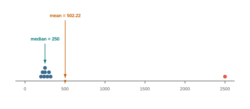
Fig. 7.7 – The effect of an outlier on the mean and median.
The right response to an outlier is to look at it, not to delete it on sight. Ask first whether it is a recording error — a mark of \(450\) in a test out of \(50\) almost certainly is, and should be corrected at the data preparation stage. But if the value is genuine, removing it means throwing away a true observation, and the honest course is to keep it and report a measure that is not distorted by it. That measure is the median, which the next subsection takes up.
7.5.1.2 Median
The median is the middle value of the data once the values have been arranged in order. Like the mean, it is computed for one attribute at a time.
To find it, sort the values in ascending or descending order. If the count is odd, the median is the value standing at the middle position. If the count is even, there is no single middle value, and the median is taken as the average of the two middle values.
Take the marks of Table 7.8 and sort them:
\[28,\ 30,\ 32,\ 38,\ 38,\ 41,\ 45,\ 45,\ 45\]
There are nine values, an odd count, so the median is the value at the fifth position, which is \(38\) — and it is the fifth value counted from either end. Four marks lie below it and four above it.
Now drop the lowest mark and consider the remaining eight:
\[30,\ 32,\ 38,\ 38,\ 41,\ 45,\ 45,\ 45\]
With an even count there is no fifth-of-nine to point at. The two middle values are the fourth and the fifth, \(38\) and \(41\), so the median is \(\dfrac{38 + 41}{2} = 39.5\). Notice that the median need not be a value that occurs in the data at all.
7.5.1.3 Mode
The mode is the value that appears the greatest number of times in the data of an attribute. It is computed from the frequency of occurrence of each distinct value.
In Table 7.8 the mark \(45\) occurs three times, \(38\) occurs twice, and each of \(28\), \(30\), \(32\) and \(41\) occurs once. The mode is therefore \(45\).
Two properties of the mode set it apart from the other two measures. First, it may not be unique: if the marks \(38\) and \(45\) had each occurred three times, the data would have had two modes. A set in which every value is distinct has no mode at all. Second, and more useful, the mode can be found for non-numeric data. You cannot compute the mean of a set of colours or the median of a set of bus routes, but you can certainly ask which colour or which route occurred most often — and for questions of that kind the mode is the only measure of central tendency available.
7.5.2 Measures of Variability
A single central value can be badly misleading on its own, because two quite different sets of data can share it. Suppose two sections of Class XII sit the same test and both return a mean of \(38\). In one section every student scored between \(35\) and \(41\); in the other, half the students scored around \(20\) and half around \(56\). The mean is honest in both cases and useless as a description of the second.
What is missing is a statement of how far the values are spread out around the centre. Measures of variability supply exactly that. They are also called measures of dispersion, since they indicate the degree of diversity within a data set, and the two commonly used ones are the range and the standard deviation.
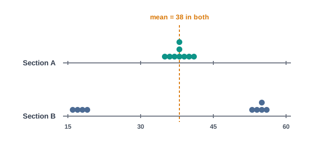
Fig. 7.8 – Two datasets with identical means but different variability.
7.5.2.1 Range
The range is the simplest measure of spread: the difference between the maximum and the minimum value in the data.
For the marks of Table 7.8, the largest value is \(45\) and the smallest is \(28\), so the range is \(45 - 28 = 17\) marks.
The range is quick to compute and easy to explain, and it tells you the total width the data cover — useful when you want to know, say, the gap between the highest and lowest fare on a route. Its weakness is the direct consequence of its definition: it is calculated from two values only, and the two it uses are the two most extreme. A single outlier therefore changes the range completely, while the behaviour of every value in between leaves it untouched. Both sections in Fig. 7.8 could be given the same range by moving one dot.
7.5.2.2 Standard Deviation
The standard deviation measures spread using every value in the data rather than just two. The idea behind it is worth following step by step, because the formula is otherwise hard to remember and easy to misapply.
Begin with the natural question: how far is each value from the mean? Compute \(x_i - \bar{x}\) for every value and you have a set of deviations. Adding them up, however, gives nothing — the positive and negative deviations cancel exactly, and the total is always zero. Squaring each deviation first removes the sign, so nothing cancels, and large deviations are weighted more heavily than small ones. Take the average of those squares, and you have a measure of spread; take its positive square root, and the measure is back in the original units of the data — marks, rupees, centimetres — rather than in squared units.
That sequence is the definition.
A small value of \(\sigma\) means the values are packed closely around the mean; a large value means they are widely spread.
Table 7.10 works it out for the marks of Table 7.8, whose mean is \(38\).
The middle column sums to zero, as it must — that is the cancellation described above, and it is a useful arithmetic check that the mean was computed correctly. The right-hand column gives what is actually needed:
\[\sigma = \sqrt{\frac{356}{9}} = \sqrt{39.5556} = 6.29\ \text{marks (to two decimal places)}\]
So the marks are spread, on average, about \(6.29\) marks either side of \(38\). For Section B of Fig. 7.8, with the same mean, the standard deviation would be far larger — which is precisely the information the mean alone could not carry.
Computing the measures in Python
Every one of these quantities is a short calculation, and writing it as a program is a useful way of checking that you have understood the method rather than memorised the formula. The algorithm below sets out the standard deviation as a sequence of steps; the program that follows computes four of the measures for the marks of Table 7.8, using nothing beyond the constructs of Class XI.
The dry run below follows the second loop, the one that accumulates the squared deviations, on the marks in their original order with mean equal to 38.0.
7.5.3 Choosing a Suitable Technique
Knowing how to compute five measures is the smaller half of the skill. The larger half is reading a situation and deciding which measure actually answers the question that was asked. The question almost always contains the clue, as Table 7.12 shows.
Three habits will get you through most such questions. Ask first whether the question is about a centre or about a spread. If it is about a centre, ask next whether the data contain extreme values, and prefer the median when they do. If the attribute is not numeric, the mode is your only option.
There is a fourth habit, harder to state as a rule but more valuable than the other three: report a measure of centre and a measure of spread together wherever you can. “The mean is \(38\) with a standard deviation of \(6.29\)” describes the class; “the mean is \(38\)” does not.
Statistical techniques of this kind are the basis of nearly all data analysis, and Python is one of the tools commonly used to apply them. Beyond the ordinary constructs used in the program above, Python offers libraries built specifically for data processing and analysis, and later chapters will take those up.
7.6 Summary
Data and information
- Data are the raw facts and figures recorded from a situation, before anyone has interpreted them. The word is a plural; its singular is datum.
- Data are not only numbers. Names, dates, transactions, images, audio, video, documents, messages and sensor readings are all data.
- Information is what data become after they have been organised, summarised and interpreted for a purpose. Data are the input; information is the output.
- The transformation deliberately loses detail. A summary answers only the question it was made for, which is why the original data are kept and not discarded once a result has been obtained.
- The value of data usually lies not in any single record but in the ability to compare, count and combine records — which is possible only because they were recorded consistently in the first place.
Structured and unstructured data
- Structured data are organised in a well defined format, normally as rows and columns. Each column holds one attribute — also called a characteristic or a variable — and each row holds the values of those attributes for one observation.
- Because a given fact always sits at a known position, structured data can be summed, sorted, counted and classified directly by a program.
- The attributes must be decided before collection begins. A fact that was never captured cannot be recovered by any later processing.
- Unstructured data are not in the traditional row-and-column structure and have no fixed format. Newspaper pages, emails, web pages, documents, images, audio and video are examples.
- Metadata are data about data — the type, size, format, origin or structure of an item rather than its content. The subject line, sender and date of an email, or the file size, file type and resolution of an image, are metadata, and they are structured even where the item they describe is not.
Data collection
- Data collection means identifying data that already exist, or gathering fresh data from an appropriate source, and recording them in a form fit for storage and processing.
- The order of work is fixed: the question to be answered decides the attributes required, which decide the source and the mode of collection, which decide how the data are recorded.
- Data may already exist on paper and need entering into digital form; may already exist digitally, for instance as a comma separated values file; or may not exist at all, in which case software must be written to capture them as they arise.
- Common modes of collecting fresh data are survey or questionnaire, interview, observation, measurement, and automatic capture by the system that generates the events.
- Collected data must be checked for relevance, accuracy, completeness and consistency. Inconsistency is the most dangerous of the four because it fails silently — the same fact recorded two different ways is counted as two different facts.
Data storage
- Data storage is the process of holding data on a storage device so that they survive the current work and can be retrieved later.
- Primary memory is fast, directly reachable by the processor, and volatile — its contents are lost when power is removed. Secondary storage is slower, not directly reachable, and non-volatile, which makes it persistent storage.
- A result computed in memory exists nowhere permanent until it is deliberately written to storage.
- Commonly used storage devices are the Hard Disk Drive (HDD), the Solid State Drive (SSD), CD/DVD, the Tape Drive, the Pen Drive and the Memory Card.
- Capacity is measured in bytes, where a byte is eight bits, and each further unit — kilobyte, megabyte, gigabyte, terabyte — is \(1024\) times the one before it. Device manufacturers often quote capacity in powers of ten instead.
- Data on a storage device are organised as files, and a program can add to, modify, delete from or read a file. This is file processing.
- File processing has limitations. The same fact stored in several files is data redundancy; when one copy is updated and another is not, the files contradict each other, which is data inconsistency. Programs must also know the exact layout of the files they read, shared access is hard to manage, and rules about what may be stored cannot be enforced by the file itself.
- These limitations can be overcome by a database management system, which stores data centrally, controls access to them, and enforces rules about what may be stored.
Data processing
- Data processing is the set of operations carried out on raw data — arranging, storing, retrieving, classifying, calculating and updating them — to produce meaningful information.
- The data processing cycle has three stages. Input covers data collection, data preparation and data entry; processing covers store, retrieve, classify and update; output covers reports and results.
- Data preparation removes duplicates, fills or flags missing fields, and makes formats and units consistent. The correctness of the output is decided at this stage, since a program cannot tell a wrong value from a right one.
- Classification is what turns a heap of records into groups from which a summary can be made; updating is what keeps stored data from drifting out of date.
- The arrangement is a cycle and not a chain, because today’s output is stored and becomes part of tomorrow’s input.
- Automated data processing, in which a computer carries out the whole cycle, is now ordinary. Any such system can be read by asking three questions of it: what is taken in, what is done, and what is produced.
Statistical techniques
- Summarisation replaces many values by a few representative ones, and is applied to structured, tabular data.
- A measure of central tendency is a single value indicating where the data are centred. The three in use are the mean, the median and the mode.
- The mean is the sum of the values divided by the number of values. It uses every value, and is therefore pulled towards any outlier — a value exceptionally large or small compared with the rest.
- The median is the middle value once the data are sorted; where the count is even it is the average of the two middle values. It divides the data into two equal parts and is almost unaffected by outliers.
- The mode is the value occurring most frequently. A data set may have no mode, one mode or several, and the mode is the only one of the three that can be found for non-numeric data.
- A central value alone can mislead, since two very different data sets can share it. Measures of variability, also called measures of dispersion, state how widely the values are spread around the mean.
- The range is the maximum value minus the minimum value. It is quick, applies only to numerical data, and depends on just two values, so a single outlier changes it completely.
- The standard deviation is the positive square root of the average of the squared differences of each value from the mean. Squaring prevents the deviations from cancelling, and the square root returns the measure to the original unit. A small value means the data are tightly clustered; a large value means they are widely spread.
- Choosing a technique starts from the question: centre or spread; if centre, whether extreme values are present; and whether the attribute is numeric at all. A measure of centre reported together with a measure of spread describes a data set far better than either alone.
7.7 Key Terms
- ATM — automated teller machine.
- Attribute — a named property recorded for every observation; in tabular data, one column. Also called a characteristic or a variable.
- Automated data processing — data processing in which a computer carries out the whole input–processing–output cycle without manual working.
- Bit — a single binary digit, 0 or 1; the smallest unit of stored data.
- Byte — a group of eight bits, historically enough to hold one character of ordinary text; the unit in which storage capacity is measured.
- CSV — comma separated values; a plain text file format in which the values of one record are written on one line, separated by commas.
- Data — the raw facts and figures recorded from a situation, before they have been processed or interpreted.
- Data collection — the process of identifying data that already exist, or gathering fresh data from an appropriate source, and recording them in a usable form.
- Data entry — the input-stage activity of putting prepared data into the system, by typing, by reading an existing file, or by automatic capture.
- Data inconsistency — the state in which copies of the same fact held in different places disagree with one another, usually because only some of them were updated.
- Data preparation — the input-stage activity of cleaning collected data before use: removing duplicates, dealing with missing fields, and making formats and units uniform.
- Data processing — the operations carried out on raw data, such as arranging, storing, retrieving, classifying, calculating and updating, in order to produce information.
- Data processing cycle — the three-stage arrangement of data processing into input, processing and output, in which the output of one round becomes stored data available to the next.
- Data redundancy — the storing of the same fact repeatedly in more than one place.
- Data storage — the process of recording data on a storage device so that they survive the current work and can be retrieved later.
- Datum — the singular form of the word data; a single recorded fact.
- DBMS — database management system; software that stores data centrally, controls access to them, and enforces rules about what may be stored.
- File — a named collection of data held on a storage device, which a program can read, add to, modify or delete from.
- GB — gigabyte; 1024 megabytes.
- HDD — hard disk drive; a storage device that holds data magnetically on rotating platters.
- ICT — information and communication technology.
- Information — the meaningful result obtained after data have been organised, summarised or interpreted for a purpose.
- JPEG — Joint Photographic Experts Group; a common image file format.
- KB — kilobyte; 1024 bytes.
- MB — megabyte; 1024 kilobytes.
- Mean — the sum of all the values of a numeric attribute divided by the number of values; also called the average.
- Measure of central tendency — a single value that represents a whole data set by indicating where its values are centred.
- Measures of variability — values indicating how widely the data are spread around the mean; also called measures of dispersion.
- Median — the middle value when the data are arranged in order; the average of the two middle values when the count is even.
- Metadata — data that describe other data, recording properties such as type, size, format or origin rather than content.
- Mode — the value that occurs most frequently in the data of an attribute.
- Outlier — a value that is exceptionally large or exceptionally small compared with the other values of the data.
- Persistent storage — storage in which data remain available after the program that created them has ended and after the machine is switched off.
- PNG — Portable Network Graphics; a common image file format.
- Primary memory — the fast, volatile memory a processor works from directly; its contents are lost when power is removed.
- RAM — random access memory; the primary memory of a computer.
- Range — the difference between the maximum and the minimum value of a numeric attribute.
- Secondary storage — non-volatile storage on which files are kept for future use; not reached directly by the processor.
- SSD — solid state drive; a storage device that holds data electronically in flash memory, with no moving parts.
- Standard deviation — the positive square root of the average of the squared differences of each value from the mean; a measure of spread that uses every value.
- Statistical techniques — methods that summarise a set of data values into a few representative values so that the data can be understood.
- Structured data — data organised in a well defined format, typically as rows and columns, with a named attribute for every column.
- Summarisation — the replacing of many data values by a few representative values, so that the data can be comprehended.
- TB — terabyte; 1024 gigabytes.
- Unstructured data — data not held in the traditional row-and-column structure, and therefore having no fixed, pre-defined format.
- USB — universal serial bus; the port through which removable devices such as a pen drive are connected.
- WWW — World Wide Web.
7.8 Points to Ponder
Metadata are structured even when the item they describe is not. If enough metadata were attached to a photograph — where it was taken, what it shows, who is in it — would the photograph become structured data? Where exactly does that argument break down?
Every summary throws away detail on purpose. Is there any summary of a data set that loses nothing at all? If not, on what grounds do you decide which details are safe to lose?
The median cannot be disturbed by an extreme value, however extreme it is. That is usually described as a strength. When would it be a weakness — that is, when would you want your summary to react to an outlier rather than ignore it?
Far more data are now produced as a by-product of systems doing their ordinary work than are gathered by deliberately asking anyone. What changes when a data set exists before anybody has decided what question it is meant to answer?
Standard deviation squares each deviation so that positive and negative differences cannot cancel. Taking the size of each deviation, ignoring its sign, would prevent cancellation just as effectively. What does squaring do that the simpler approach does not?
File processing has known limitations, and a database management system exists to overcome them — yet a great deal of data in the world is still kept in ordinary files. What does that suggest about when a limitation is worth the cost of removing it?
7.9 Objective Questions
The singular form of the word “data” is
- datas
- datum
- datae
- datar [1 mark]
Which one of the following is an example of unstructured data?
- A bus reservation chart
- A stock register kept in a spreadsheet
- The body of an email message
- A table of marks stored in a database [1 mark]
Which measure of central tendency can be found for non-numeric data such as the colours of cars in a parking area?
- Mean
- Median
- Mode
- Standard deviation [1 mark]
Fill in the blank: The difference between the maximum and the minimum value of a numeric attribute is called its ____________. [1 mark]
State whether the following statement is true or false: The median of a data set is always one of the values present in that data set. [1 mark]
Assertion (A): The mean is not a suitable summary when the data contain an outlier. Reason (R): The mean is computed using every value in the data set.
- Both A and R are true, and R is the correct explanation of A.
- Both A and R are true, but R is not the correct explanation of A.
- A is true but R is false.
- A is false but R is true. [1 mark]
Assertion (A): Storing a student’s address in three separate departmental files is an instance of data redundancy. Reason (R): Keeping several copies of a fact guarantees that the fact will always be correct.
- Both A and R are true, and R is the correct explanation of A.
- Both A and R are true, but R is not the correct explanation of A.
- A is true but R is false.
- A is false but R is true. [1 mark]
Match each measure in Column I with what it reports in Column II.
| Column I | Column II |
|---|---|
| a. Mean | i. The value occurring most often in the data |
| b. Median | ii. The spread of the data computed from every value |
| c. Mode | iii. The sum of the values divided by their count |
| d. Range | iv. The largest value minus the smallest value |
| e. Standard deviation | v. The middle value once the data are ordered |
[1 mark]
- Write the full form of each of the following abbreviations: CSV, DBMS, ICT, SSD. [1 mark]
7.10 Check Your Concepts
Define metadata, and give one example of metadata for a file other than an email. [2 marks]
Distinguish between data and information in two points. [2 marks]
Why must the values be sorted before the median is picked out? State what a program would report if this step were left out. [2 marks]
Differentiate between structured data and unstructured data on any three points, giving one example of each. [3 marks]
What is meant by data preparation? Describe any three checks carried out at this stage, with one short example for each. [3 marks]
Explain the three stages of the data processing cycle, naming the activities that belong to each stage, and state why the arrangement is described as a cycle rather than as a chain. [4 marks]
The number of books issued from a school library on seven working days was 12, 15, 11, 15, 60, 14 and 15. Find the mean, the median, the mode and the range of this data. State which measure best describes a typical day’s issue, and give your reason. [4 marks]
Two sections of Class XII obtain exactly the same mean marks in a test, yet their performances are described as very different. Explain what measures of variability are, define range and standard deviation, and give two reasons why the standard deviation is the better measure to report here. State the pair of values you would quote to describe each section. [5 marks]
A school keeps its student details separately in the office file, the examination file and the transport file. Explain, with an illustration drawn from this situation, what data redundancy and data inconsistency mean, state any two further limitations of file processing, and name the kind of software used to overcome them. [5 marks]
7.11 Output & Debugging
- Predict the exact output of the following code, and then state whether the second line printed is the median of the list. Justify your answer.
values = [4, 8, 15, 16, 23, 42]
n = len(values)
print(sum(values) / n)
print(values[n // 2])
[2 marks]
- The following code is intended to print the median of the list. State the output it actually produces, identify the single error in it, and write the corrected code.
data = [50, 12, 39, 21, 8]
middle = len(data) // 2
print("Median:", data[middle])
[3 marks]
- The following code raises an error when it is run. Name the error, explain why it occurs, and rewrite the code so that it works as intended.
readings = [22, 27, 19, 31, 25]
range = max(readings) - min(readings)
for i in range(2):
    print(readings[i])
[3 marks]
- Write the exact output of the following code, and state which measure of central tendency this code helps to determine.
marks = [18, 25, 25, 30, 25, 18]
counts = {}
for m in marks:
    counts[m] = counts.get(m, 0) + 1
print(counts)
[3 marks]
- In one file of a school, the date of admission is recorded as 05-04-2026, while in another file the same admission is recorded as 2026-04-05. A program that counts admissions month by month reports two different totals depending on which file it reads. Name the data quality problem involved, state the stage of the data processing cycle at which it should have been caught, and explain why no error message is produced. [3 marks]
7.12 Case-Based Questions
- A science laboratory register records the temperature, in degrees Celsius, noted at the end of six trials of the same experiment. The recorded data are shown in Table 7.13.
a. Compute the mean and the range of the six recorded values. [2 marks]
b. Name the kind of value that T3 represents, and state how it should be dealt with at the data preparation stage, giving your reason. [1 mark]
c. If the value at T3 could not be verified and had to be retained, which measure of central tendency should be reported for this data, and why? [1 mark]
[4 marks]
- The transport in-charge of a school maintains the record shown in Table 7.14 for the four school buses, noting for each bus the route, the number of students boarding it, the distance covered and the delay in its arrival at the school on a particular day.
a. State whether this record is structured or unstructured data, giving two reasons drawn from the table itself. [2 marks]
b. The in-charge wants to know whether the four buses are about equally punctual or whether their punctuality varies widely. Name the statistical technique that answers this, and justify why the measure you have chosen is more suitable here than a measure of central tendency. [2 marks]
c. The in-charge later wants to know at what time each bus started from its first stop, but finds that this cannot be worked out from the record. Explain what has gone wrong and at which stage of the work the mistake was made. [1 mark]
[5 marks]
7.13 Programming Practice
Write a complete Python program that stores the daily maximum temperature of a week in a list and displays the mean, rounded to two decimal places, and the range of the week’s temperatures. Submit the complete program together with an identifier description table listing every identifier used, its type and its purpose. Test the program on the list
[34, 34, 27, 28, 27, 34, 34]and show the output produced. [4 marks]Write a Python function that accepts a list of numeric values as its argument and returns the median of that list, working correctly whether the number of values is odd or even. The function must not alter the order of the list that was passed to it. Submit the function definition, two calls that demonstrate both cases, and a two-line note stating why sorting is essential to the method and why the original list is left unchanged. [5 marks]
Write a complete Python program that stores the marks of ten students in a list and displays the standard deviation of those marks, rounded to two decimal places, without using any library or module. The program must first compute and display the mean, and must then use it to accumulate the squared deviations. Submit the program and state, in one line, what would go wrong if the mean and the squared deviations were accumulated in a single pass over the list. [4 marks]