Chapter 9: Structured Query Language (SQL)
Until the early 1970s, getting a single fact out of a large collection of stored data was a programming job. If a clerk wanted the address of one customer, a programmer had to write instructions that opened the right file, moved through it record by record, followed pointers from one block of storage to the next, and stopped when the record matched. Change the way the data was stored, and every one of those programs had to be rewritten.
In 1970, Edgar F. Codd, working at IBM’s San Jose research laboratory, published a paper in Communications of the ACM proposing a different arrangement. Store the data as simple tables of rows and columns, he argued, and let a person ask for what they want by describing it — leaving the machine to work out how to find it.
IBM built an experimental system, called System R, to test whether the idea would actually work. For it, Donald D. Chamberlin and Raymond F. Boyce designed a language whose statements read almost like English sentences. They called it SEQUEL, short for Structured English Query Language; the name was later shortened to structured query language (SQL). It became an American national standard in 1986 and an international one the following year.

Fig. 9.0 – Telling the machine how to search versus what to search for.
Today almost every relational database — a school’s records, a shop’s stock, a railway reservation list — is questioned in this language.
This chapter will answer each of these questions.
9.1 Why a Database Needs a Query Language
Every school office keeps records, and for a long time it kept them on paper. Admission details sat in one register, fee receipts in a second, attendance in a third, and the library’s issue slips in a fourth. Each register was perfectly readable on its own. The difficulty appeared the moment someone asked a question that crossed two of them — which students who joined this year have not returned a library book? — because answering it meant opening two registers side by side and matching entries by hand.
Storing the same records in a computer removes the paper, but it does not by itself remove that difficulty. What removes it is a particular way of arranging the data, together with a particular way of asking questions of it. This section looks at both, because everything the rest of the chapter does rests on them.
Data Kept in Files
Suppose the admission records are kept in an ordinary file, one line per student. To find a single student’s details, a program has to open the file, read a line, compare it with what was asked for, and move on to the next line if it does not match. The program stops when it finds the record or when the file runs out.
That works. But notice what the programmer has had to know: which file the data is in, what order the fields appear in, where one field ends and the next begins, and how to walk through the file from start to finish. All of that knowledge sits inside the program. Change the layout — insert a new field, split one file into two — and every program that touched the file has to be found and corrected.
Notice also what the file itself does not do. Nothing in the file stops two students being given the same roll number. Nothing stops a date of birth being stored as 31-02-2007. Nothing links a fee receipt to the student it belongs to except a number that both records happen to contain, and the matching has to be programmed by hand each time. Correctness is entirely the programmer’s responsibility, repeated in every program.
Data Kept as Relations
The alternative you met in the previous chapter is to store the data as a database — an organised collection of related data, held so that it can be retrieved and updated as required — and to arrange that data according to the relational data model.
In this model all data is held in relations. A relation is a table with a fixed set of named columns and any number of rows. Each row is a tuple, and holds the facts about one thing. Each column is an attribute, and holds one kind of fact about every thing in the table. Table 9.1 shows a small relation recording a school’s bus routes.
Two counts describe the size of a relation, and it is worth keeping them apart. The degree of a relation is the number of attributes it has; BUSROUTE has degree 4. The cardinality of a relation is the number of tuples it holds; BUSROUTE has cardinality 5. Degree is fixed by the design of the table and changes only when the school decides to record something new about a route. Cardinality changes every time a route is added or withdrawn. The anatomy of the relation is set out in Fig. 9.1.
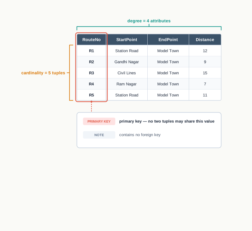
Fig. 9.1 – The BUSROUTE relation.
One attribute in Table 9.1 does a special job. No two routes may carry the same RouteNo, so knowing the route number is enough to pick out exactly one tuple. An attribute that identifies each tuple uniquely in this way is the relation’s primary key. A primary key may never be left blank and may never repeat, because a value that is missing or shared would identify nothing.
Now suppose the school also records each daily trip: a trip number, the route the trip ran on, and its departure time, in a second relation BUSTRIP with attributes TripNo, RouteNo and DepartureTime. The RouteNo in BUSTRIP is not there to identify the trip; it is there to point at a route in BUSROUTE. An attribute in one relation that refers to the primary key of another relation is a foreign key, and it is what allows a question to travel from one table to the other. Fig. 9.2 shows the reference.
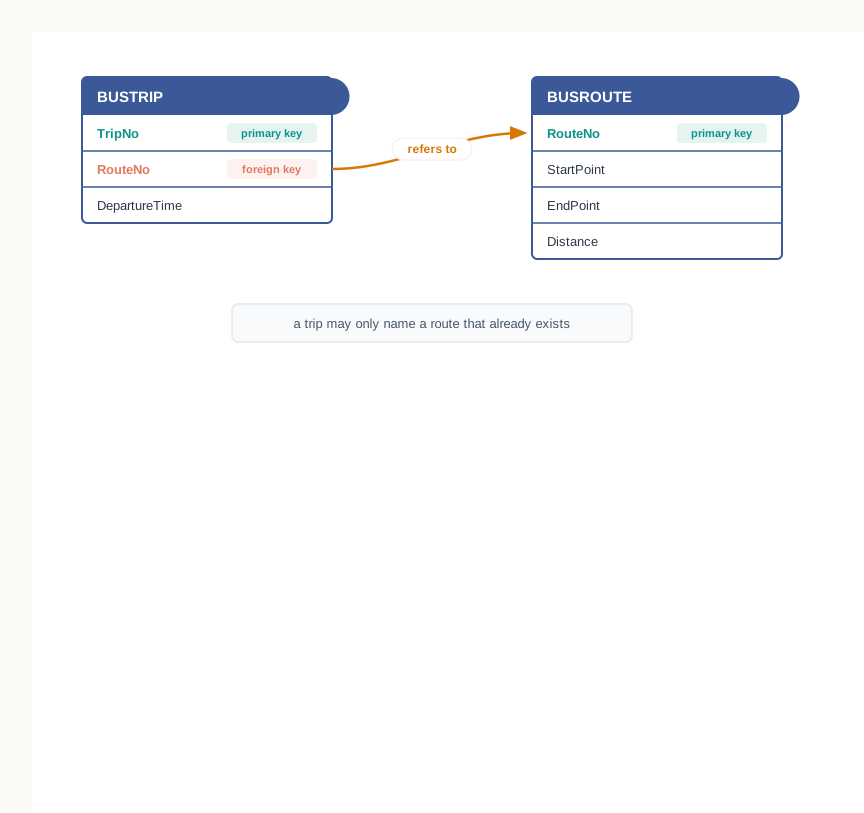
Fig. 9.2 – Foreign key reference between BUSTRIP and BUSROUTE.
Asking a Question of the Data
A request made to a database is called a query. The important thing about a query is what it does not contain. It does not say which file to open, in what order to read the rows, or when to stop. It states the data wanted — the route numbers of all routes longer than ten kilometres, in descending order of distance — and leaves the method of finding them entirely to the database software. The language in which such requests are written is a query language.
The path a request takes is shown in Fig. 9.3. You write a query and hand it to the database management system; the system works out how to satisfy it, reaches into the stored data, and hands back the answer — itself in the form of a table.
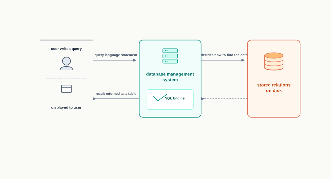
Fig. 9.3 – The path of a database request.
This is a genuine shift in who does what, and it is worth setting the two arrangements against each other directly.
The Software That Answers the Question
The software that stores the relations, enforces the rules declared on them and answers the queries is a relational database management system (RDBMS). MySQL, PostgreSQL, Oracle and Microsoft SQL Server are all systems of this kind. They differ in how they are installed, licensed and tuned, but a query written for one is largely recognisable in another, because they answer to the same query language and the same underlying model.
Throughout this chapter the system used is MySQL, and every statement shown is one you can type at its prompt and run. What you will build up, section by section, is the ability to describe a table, fill it with data, correct that data, and then put questions to it — first simple ones, then questions that summarise, group and combine.
9.2 Structured Query Language
The previous section argued that a database needs a language in which questions can be stated rather than programmed. Relational systems settled on one such language, and it has stayed remarkably stable ever since. Its statements are built out of ordinary English words — SELECT, FROM, WHERE, INSERT, DELETE — arranged so that a well-written statement can almost be read aloud as a sentence.
Because it is an international standard, the same core language works across relational systems. A statement written for one system will usually run unchanged on another, and a student who learns it on one system has not learnt a single product but a skill that travels. Each system does add extensions of its own, so a statement that uses a system’s private features may not carry across; the material in this chapter stays close to the common core.
9.2.1 What SQL Lets You Do
Recall the central promise from Section 9.1: you describe the data you want, and the system works out how to get it. This is exactly what SQL does. A request such as give me the names and distances of routes longer than ten kilometres, longest first becomes a short statement naming the columns wanted, the table they come from, the condition the rows must satisfy and the order the answer should appear in. Nowhere does the statement say how to search, in what order to examine the rows, or where on the disk to look.
The name says “query”, but SQL does considerably more than ask questions. Everything you will do to a database in this chapter is done in the same language, and the work falls into four kinds:
- Defining structure — creating a database and its tables, naming each column, fixing what kind of value it may hold, and changing that structure later when the design turns out to need it.
- Declaring rules — stating that a column must never be blank, that its values must never repeat, or that its value must match a value already present in another table.
- Storing and changing data — inserting new rows, correcting values in existing rows, and removing rows that are no longer wanted.
- Retrieving data — selecting rows and columns, ordering them, summarising them into counts and totals, grouping them, and drawing together data held in more than one table.
The first two kinds shape the container; the last two work on what the container holds. Sections 9.4 to 9.11 take them in that order, because you cannot put a row into a table that does not exist yet, and you cannot ask a question of data you have not stored.
9.2.2 Working at the MySQL Prompt
The system used throughout this chapter is MySQL. It is open source software, meaning its source code is published and it may be downloaded and used free of cost, which is why it is the system most school laboratories install.
Once MySQL is installed and its service is running, you reach it through a client program that gives you a prompt. When the prompt reads mysql>, as shown in Fig. 9.4, the system is waiting for a statement.
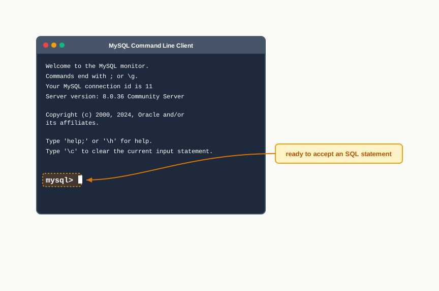
Fig. 9.4 – The MySQL command-line client.
Three habits of the prompt are worth fixing at the start, because every statement in this chapter depends on them.
Every statement ends with a semicolon
The semicolon is how you tell the client that you have finished typing. Pressing Enter is not enough — the client assumes you have more to type and waits. This is not a nuisance; it is what makes it possible to spread a long statement over several lines.
Long statements may run over several lines
If you press Enter before the semicolon, the prompt changes from mysql> to ->, indicating that the statement is being continued. You may keep typing on the new line, and the statement is only sent when the semicolon finally arrives. Queries in this chapter are often laid out over three or four lines for exactly this reason, with each clause on a line of its own so that the shape of the statement is visible at a glance.
Keywords and column names are not case-sensitive
SELECT, select and Select are the same word to SQL, and the column names distance and DISTANCE refer to the same column. The convention followed in this book — keywords in capitals, table and column names as they were declared — is for the reader’s benefit, not the system’s. One qualification matters: database names and table names may or may not be case-sensitive, depending on the operating system the server runs on. They are treated as distinct on most Linux systems and as the same on Windows. The safe practice, and the one this chapter follows, is to write a database or table name in exactly the letter case in which it was created.
The transcript below shows all three at work. The statements are arithmetic rather than anything about a table, because at this point no table exists — but they are complete, valid SQL, and the system answers them as it answers any other query.
mysql> SELECT 2+3;
+-----+
| 2+3 |
+-----+
|   5 |
+-----+
1 row in set (0.00 sec)

mysql> SELECT 12*7,
    -> 100-45;
+------+--------+
| 12*7 | 100-45 |
+------+--------+
|   84 |     55 |
+------+--------+
1 row in set (0.00 sec)
Notice the second statement. Enter was pressed after the comma, the prompt became ->, the rest of the statement was typed on the next line, and only the semicolon sent it. Notice also that the answer came back as a table with a column heading — even here, where the question had nothing to do with any stored data. Every SQL query returns a table, and that fact will matter later, when the result of one query becomes something you can question further.
From here on, the queries in this chapter are shown as statements on their own, without the mysql> prompt in front of them, and their results are shown as ordinary tables rather than as screen transcripts. That is only a matter of presentation on the page. What you type at the prompt is exactly what is printed, semicolon included.
9.3 Data Types and Constraints in MySQL
A relation is not merely a grid of values. Before a single row can be stored, the database has to be told what each column is for: what kind of value it will hold, and what values it must refuse. These two decisions — the data type of a column and the constraints placed on it — are taken when the table is designed, and they are difficult to undo once thousands of rows depend on them. This section deals with the decisions themselves; Section 9.4 shows the statements that carry them out.
9.3.1 Data Type of an Attribute
Section 9.1 said that the values in a column are drawn from a single domain — all distances, all names, all dates of birth. The data type of an attribute is how that domain is stated to the database in a form it can enforce.
Fixing a data type settles two things at once. It settles what may be stored: a column declared to hold dates will not accept the word “Monday”. It also settles what may be done with what is stored: you may add and average the values in a numeric column, but adding two names is meaningless, and the system will not pretend otherwise. Choosing a type is therefore not book-keeping — it is the first decision that protects the data.
MySQL offers a large collection of types, grouped broadly into numeric types, string types, and date and time types. Table 9.3 lists the ones this chapter uses.
Two of these need a further word. For whole numbers larger than INT can hold, MySQL provides BIGINT, which occupies 8 bytes. And where a fractional number must be exact rather than approximate — an amount of money, for instance — FLOAT is the wrong choice; the type meant for that purpose is DECIMAL, which stores a stated number of digits before and after the decimal point exactly as written. Every money amount in this chapter is kept in whole rupees, so INT serves.
Fixed length or varying length
The choice that causes most difficulty is between CHAR(n) and VARCHAR(n), because both hold text and both take a length. The difference is in what happens to the unused space, and Fig. 9.5 shows it directly.
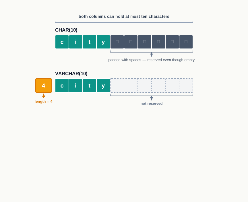
Fig. 9.5 – Storage of CHAR(10) versus VARCHAR(10).
In a CHAR(10) column, the word city occupies all ten character positions — four letters and six spaces. In a VARCHAR(10) column the same word occupies the four letters and a small marker recording that the length is four. The cost of VARCHAR is that marker and a little extra work while reading; the cost of CHAR is the wasted space, which becomes real when the column is wide and the values are short.
So a column recording attendance as 'P' or 'A' is naturally CHAR(1); a column recording a guardian’s address is naturally VARCHAR(30) or wider, since addresses differ enormously in length.
The same reasoning applies to any identifier built out of digits — a roll number that is genuinely counted and compared is a number, while a twelve-digit code that merely names something is text.
9.3.2 Constraints on an Attribute
A data type rules out values of the wrong kind, but it cannot rule out values of the right kind that are still wrong. Nothing about the type INT prevents two students being given the same roll number, and nothing about VARCHAR(20) prevents a student’s name being left out altogether. Rules of that sort are stated separately, as constraints.
The word “enforces” is the whole point. A constraint is not a note to the programmer; it is a rule the database itself applies, to every statement, from every user, for as long as the table exists. A check written inside one program protects only that program. A constraint protects the data.
Before the constraints themselves, one value needs naming. When a column of a row has no value at all — the fact is missing, unknown, or does not apply — the database records a null value, written NULL. It is not zero, and it is not an empty piece of text; it is the recorded absence of a value. Unless something forbids it, any column may hold NULL. Table 9.5 lists the constraints used in this chapter.
Declaring constraints is not compulsory. A table with none at all will be created quite happily, and will then accept whatever is put into it. What you lose is every guarantee about the data — and guarantees, once lost, are almost impossible to restore from thousands of existing rows.
Three of the entries in Table 9.5 repay a closer look.
The primary key says more than “unique”
A primary key carries two guarantees at once: values never repeat, and values are never null. There is a further condition that is easy to overlook — a table may have at most one primary key. That is not a limitation but the point of the thing. The primary key is the declaration of how a row of this table is to be identified, and a table cannot have two different answers to that question. A key may, however, be built from more than one column together, which Section 9.4.4 takes up.
A foreign key points outward
NOT NULL, UNIQUE and DEFAULT are rules about a column on its own. A foreign key is different: it is a rule about the relationship between two tables. Declaring RouteNo in a trip table as a foreign key referring to the route table means the database will refuse a trip that names a route which does not exist. The nonsense record is rejected at the moment someone tries to create it, rather than being discovered months later by a query that returns something impossible.
A foreign key column may itself hold NULL unless it has also been declared NOT NULL. That is deliberate, and it is often what you want: a null in a foreign key means not yet linked to anything, which is a legitimate state, while a wrong value means linked to something that does not exist, which never is.
Unique columns and the null value
One subtlety follows from the two ideas together. A UNIQUE column forbids repeated values, but in MySQL more than one row may still hold NULL in it — because two unknown values are not known to be equal, and the system will not pretend they are. So a guardian’s phone number column may be UNIQUE and still be blank for several guardians. If that is not wanted, the column needs NOT NULL as well.
9.4 SQL for Data Definition
Nothing can be stored until there is somewhere to store it. Before a single row of data exists, the database has to be told that a relation exists, what it is called, what its attributes are called, what type of value each attribute holds and what rules the values must obey. That description is the relation’s schema, and the statements that create it, change it and remove it are known together as the data definition language (DDL).
Two habits of mind are worth carrying into this section. The first is that a schema is a design decision, not a formality — a badly chosen column will still be there, holding thousands of rows, long after the person who chose it has left. The second is that a schema is not permanent. It can be altered, and this section shows how; but altering a live schema is always more trouble than getting it right the first time.
The database this chapter will build
Everything from here to the end of the chapter uses one small database, called SchoolLibrary. It has three relations, shown in Fig. 9.6: MEMBER, holding one row per member of the library; BOOK, holding one row per title the library owns; and ISSUE, holding one row for each occasion on which a book was issued to a member.
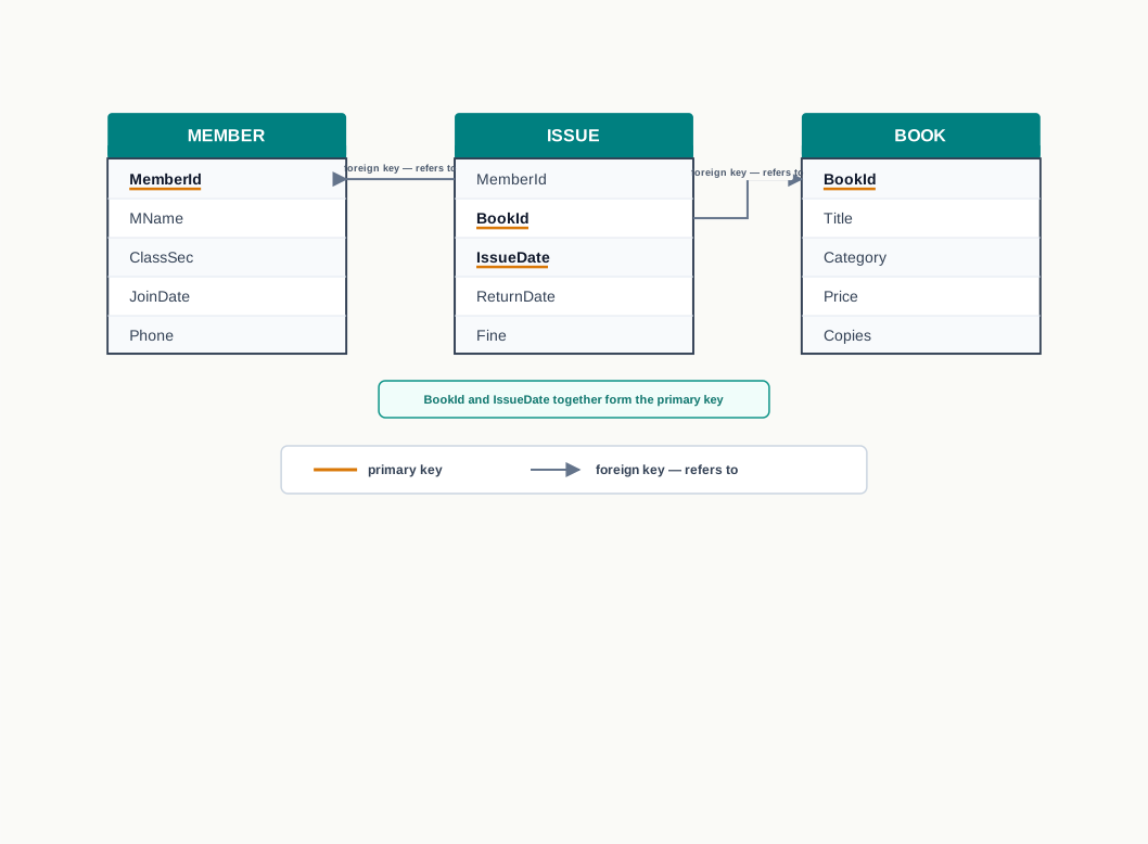
Fig. 9.6 – Schema diagram of the SchoolLibrary database.
Notice how the three relations divide the facts. A book’s price is a fact about the book, so it lives in BOOK and is recorded once however many times the book is issued. A member’s class is a fact about the member. The date on which a particular book went out to a particular member is a fact about neither on its own — it is a fact about the pairing, and so it lives in ISSUE. Getting facts into the table they belong to is most of what table design is.
9.4.1 Creating and Selecting a Database
A single MySQL server can hold many databases side by side — one for the library, another for the fee records, another belonging to somebody else’s project altogether. So there are two steps: bringing a database into existence, and then saying which one you intend to work in.
MySQL confirms that the database has been created. To see the databases already present on the server, use:
SHOW DATABASES;The list that comes back includes SchoolLibrary along with several databases MySQL maintains for its own purposes — leave those alone. Creating a database does not put you inside it; you must select it:
USE SchoolLibrary;MySQL replies that the database has changed, and from that moment every table you create or question is looked for inside SchoolLibrary. Forgetting this step is a common source of puzzlement: a statement that refers to a table by name will fail, not because the table is missing, but because you are standing in the wrong database.
A newly created database is empty, and you can confirm it:
SHOW TABLES;The result is an empty set. Now there is something to fill.
9.4.2 Creating a Table
The statement that creates a relation lists its attributes one after another, each with its data type and, if you wish, the constraints it must obey. Before writing one, though, it is worth being clear about what the statement is being asked to express.
Read that statement against the design steps. MemberId is a number that is genuinely counted, so INT; it identifies a member, so it is the primary key. MName varies in length and must always be known, so VARCHAR(20) NOT NULL. ClassSec holds values like 12A — always exactly three characters — so CHAR(3); it is left nullable because a member may be a member of staff rather than a student. JoinDate is a genuine date and is always known. Phone is exactly ten characters of digits, and for the reasons given in Section 9.3.1 it is text, not a number.
The structure that resulted can be inspected with the DESCRIBE statement, which may also be shortened to DESC:
DESCRIBE MEMBER;Three things in Table 9.6 deserve a moment. The Null column says NO for MemberId even though nothing in the statement said NOT NULL — declaring it the primary key was enough, because a primary key may never be null. The Key column marks it PRI. And the Default column reads NULL throughout, meaning that a row inserted without a value for one of these columns will hold a null there, if the column allows it.
The second table is created the same way, with the primary key written beside the attribute instead of on a line of its own. Both forms are correct; the separate line is needed only when the key is built from more than one attribute.
CREATE TABLE BOOK(
    BookId CHAR(4) PRIMARY KEY,
    Title VARCHAR(30) NOT NULL,
    Category VARCHAR(12),
    Price INT,
    Copies INT);
The third table is different, and deliberately so. ISSUE is created with its attributes and its NOT NULL rules, but with no keys at all:
CREATE TABLE ISSUE(
    BookId CHAR(4) NOT NULL,
    MemberId INT NOT NULL,
    IssueDate DATE NOT NULL,
    ReturnDate DATE,
    Fine INT);
ReturnDate is left nullable on purpose: while a book is still out, there is no return date, and a null is the honest way to record that. Fine is nullable for the same reason. The keys are left out so that the next section can show the statements that add them — and because when several related tables are being built, the foreign keys genuinely do have to wait until the tables they point at exist.
9.4.3 Viewing the Structure of a Table
DESCRIBE has already appeared, and it is worth naming what it is for. It does not show you any data; it shows you the shape the data must fit. When a statement is rejected and you cannot see why — a value too long, a column that will not accept a null, a name spelt differently from the way you remember — DESCRIBE is the first thing to run, because it answers all three questions at once.
SHOW TABLES; complements it. Where DESCRIBE reports on one table, SHOW TABLES lists the tables the current database now contains. Run at this point, it lists the three tables just created. Whether their names appear in the letter case in which you created them, or entirely in lower case, depends on the operating system the server runs on, for the reason given in Section 9.2.2.
9.4.4 Altering a Table
A table’s structure can be changed after it has been created, and the statement that does it is ALTER TABLE. The uses are various — adding a key that was left out, adding a constraint the design turned out to need, adding a column for a fact nobody thought of, widening a column that proved too narrow, removing a column that is no longer wanted — but they all follow one general form.
The sub-sections that follow take these forms one at a time, and by the end of them the SchoolLibrary schema is complete.
9.4.4.1 Adding a Primary Key
ISSUE was created without a primary key, and it needs one. Which attribute identifies a row? Not BookId, because the same book is issued many times. Not MemberId, because the same member borrows many books. Not IssueDate, because several books go out on the same day.
But BookId and IssueDate taken together do identify a row: the library does not issue the same title twice on the same day. A primary key built from two or more attributes in this way is a composite primary key.
ALTER TABLE ISSUE
ADD PRIMARY KEY (BookId, IssueDate);
The guarantee a composite key gives is about the combination, not about either attribute on its own. BookId may repeat freely down the column, and IssueDate may repeat freely, but no two rows may agree on both at once. Every attribute taking part in a primary key must also be NOT NULL, which is why both were declared that way when the table was made.
9.4.4.2 Adding a Foreign Key
ISSUE now identifies its rows, but nothing yet stops it recording an issue of a book that the library does not own, or to a member who does not exist. The foreign keys do that.
Three conditions must hold before a foreign key can be declared, and all three follow from what a foreign key means:
- The referenced table — the table being pointed at — must already exist. You cannot refer to something that has not been made.
- The referenced attribute must be the primary key of that table, or part of it. A reference has to land on something that identifies a row uniquely, otherwise it would be ambiguous.
- The referencing and referenced attributes must have the same data type and size.
CHAR(4)may refer toCHAR(4); it may not refer toINT.
With those satisfied, both keys can be added:
ALTER TABLE ISSUE
ADD FOREIGN KEY (BookId) REFERENCES BOOK(BookId);
ALTER TABLE ISSUE
ADD FOREIGN KEY (MemberId) REFERENCES MEMBER(MemberId);ISSUE is now the referencing table for both BOOK and MEMBER. From this point onwards the database itself refuses nonsense, as Fig. 9.7 shows: an attempt to record an issue of book B999, when no such book exists in BOOK, is rejected at the moment it is made rather than discovered later by a query that returns something impossible.
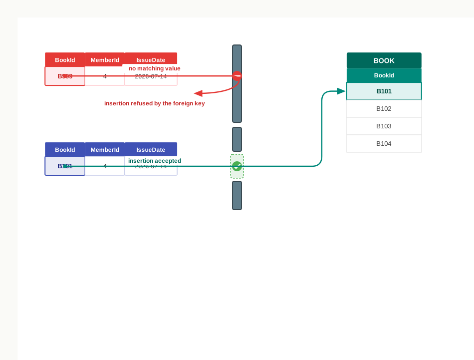
Fig. 9.7 – A foreign key constraint rejecting an invalid insertion.
Both BookId and IssueDate are marked PRI, which is how a composite key shows itself — two attributes sharing one key. MemberId is marked MUL, meaning values may repeat in that column, as they must: a member borrows more than one book.
9.4.4.3 Adding the UNIQUE and DEFAULT Constraints
Suppose the librarian now points out that two members must never be recorded with the same phone number, since duplicate numbers are how the same person ends up with two membership cards. That is a UNIQUE constraint, and it can be added to the existing table:
ALTER TABLE MEMBER
ADD UNIQUE (Phone);
The statement succeeds only if the data already in the table obeys the new rule. If two members are already sharing a number, MySQL refuses to add the constraint, and it is right to: a rule the stored data breaks is not a rule.
A default value is added differently, because it belongs to the definition of the attribute rather than to the table. Most titles arrive as a single copy, so Copies may sensibly default to 1:
ALTER TABLE BOOK
MODIFY Copies INT DEFAULT 1;
Note that the data type had to be written again. MODIFY does not adjust part of an attribute’s definition — it replaces the definition entirely, which is why the type must be restated every time. The next section but one shows what happens when that is forgotten.
9.4.4.4 Adding and Removing an Attribute
An attribute can be added to a table that already holds data. The new column appears at the end, and every existing row is given a null in it, since no value was ever supplied:
ALTER TABLE BOOK
ADD Shelf CHAR(2);
Removing an attribute is the mirror image, and it is worth pausing over, because the two statements are not equally forgiving. Adding a column costs a little space. Removing one destroys every value in it, in every row, with nothing kept in reserve:
ALTER TABLE BOOK
DROP Shelf;
The library, as it happens, moved to open shelves and no longer records shelf positions, so Shelf goes and BOOK returns to five attributes. Had the column contained a year of carefully entered data, that single statement would have ended it.
9.4.4.5 Modifying the Data Type of an Attribute
Titles turned out to be longer than the thirty characters allowed for them, so the column is widened:
ALTER TABLE BOOK
MODIFY Title VARCHAR(40) NOT NULL;
Widening a column is safe: every value that fitted in thirty characters fits in forty. Narrowing is not. If the column were reduced to VARCHAR(10) while titles longer than ten characters were stored, MySQL would refuse the change rather than quietly cut the values short. Changing a type altogether — text to a number, say — carries the same risk, and should be done only when you know what every stored value would become.
9.4.4.6 Removing a Primary Key
A primary key can also be dropped, and the statement is short. Before running it, though, make a table to run it on — testing a destructive statement on a table that matters is a habit best never formed:
CREATE TABLE MAGAZINE(
    MagId INT PRIMARY KEY,
    MagName VARCHAR(20) NOT NULL,
    Frequency VARCHAR(10));
ALTER TABLE MAGAZINE
DROP PRIMARY KEY;Notice that no attribute is named in the second statement. A table has at most one primary key, so there is nothing to choose between. Nothing refers to MAGAZINE, so its key comes away freely — and once it is gone, nothing prevents two rows carrying the same MagId.
There is a reason that example does not name one of our three tables. Try the same statement on BOOK, and MySQL refuses it, reporting that the index concerned is required by a foreign key constraint. ISSUE points at BookId, and removing what it points at would leave the reference dangling. The same applies to MEMBER. Far from being an obstruction, this is the database defending the design: once other tables depend on a key, that key is not yours to remove casually.
Title is now forty characters wide and still NOT NULL; Copies carries a default of 1; Shelf has gone without trace. The schema drawn in Fig. 9.6 is complete.
9.4.5 Dropping a Table and a Database
The scratch table has served its purpose and can go.
DROP cannot be undone. There is no confirmation, no recycle bin and no partial version — the table is simply not there any more, and the only way back is from a backup taken beforehand. For that reason, running SHOW TABLES; and reading the name you are about to type is not timidity; it is ordinary care.
MySQL does provide one protection. A table that another table’s foreign key refers to cannot be dropped while the reference exists: DROP TABLE BOOK; would be refused for exactly the reason given in Section 9.4.4.6. The reference has to be removed first, deliberately, which is one more decision than an accident usually survives.
SchoolLibrary now contains three tables with a settled structure and not one row of data. Filling them is the business of the next section.
## 9.5 SQL for Data Manipulation


At the end of Section 9.4 the `SchoolLibrary` database had three tables with a settled structure and no data whatever. Creating a table creates only the container; the rows have still to be put in, corrected when they are wrong, and removed when they are no longer wanted.

The statements that do this work — `INSERT`, `UPDATE` and `DELETE`, together with the `SELECT` statement that retrieves data — form the **data manipulation language (DML)**. The distinction between this and the data definition language of the previous section is worth fixing, because it is the difference between changing the shape of the container and changing what is inside it.

::: {.callout-note .box-compare icon=false title="Compare Table" collapse="true"}

Table 9.9 – Data definition language and data manipulation language
| Feature | Data definition language | Data manipulation language |
|---|---|---|
| What it changes | The structure of the database — tables, attributes, keys, constraints | The data held inside the tables — the rows |
| Statements used here | `CREATE`, `ALTER`, `DROP` | `INSERT`, `UPDATE`, `DELETE`, `SELECT` |
| Typical frequency of use | Rarely, mostly when the database is designed or redesigned | Constantly, every day the database is in use |
| Who normally writes it | The person designing the database | Anyone using it, including programs written by others |
| Effect on existing rows | May reshape or destroy them wholesale | Adds, changes or removes rows one group at a time |

:::


This section deals with putting rows in. Correcting and removing them is taken up in Section 9.7, after the `SELECT` statement has been met, because you cannot sensibly change a row until you can see it.

##### The order in which tables are filled {.unnumbered .unlisted}


The three tables of `SchoolLibrary` cannot be filled in any order you please. ISSUE holds foreign keys pointing at BOOK and at MEMBER, and a foreign key value must already exist in the table it refers to. Trying to record an issue before the book is on the shelf is not a technicality — it is a statement about a book the library does not own.

::: {.callout-note .box-algorithm icon=false title="Algorithm" collapse="true"}

populating a set of related tables
Input: rows to be inserted into several tables, some of which hold foreign keys referring to others.
Output: all the rows stored, with every foreign key matching an existing value.
Method:
```text
1. List the tables and, for each one, the tables its foreign keys point at.
2. Fill first every table that has no foreign key at all.
3. Take any table all of whose referenced tables are now filled, and fill it.
4. Repeat step 3 until no table is left.
Why it works: at the moment any row is inserted, every table its foreign keys refer to has already been filled, so every reference finds a match. Watch out: if two tables refer to each other, no order works and the design itself has to be reconsidered — usually by allowing one of the foreign keys to be null at first and filling it in later.
:::
Applying this to SchoolLibrary gives the order shown in Fig. 9.8: BOOK and MEMBER in either order, and ISSUE last.
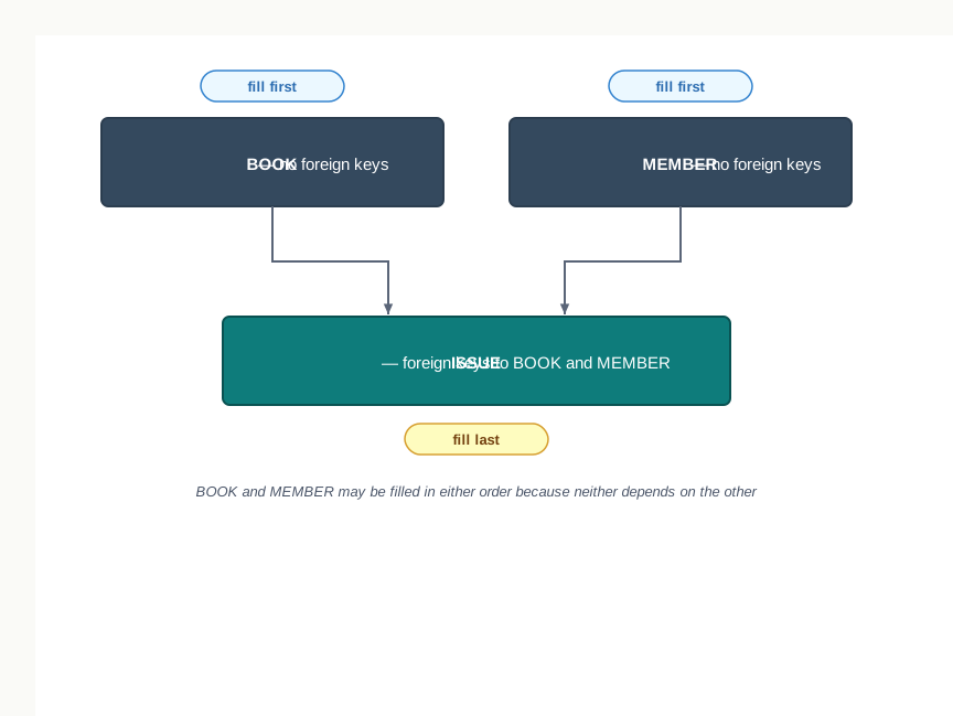
Fig. 9.8 – Order of filling related tables.
9.5.1 Inserting a Complete Record
The INSERT INTO statement adds one row to a table. In its simplest form it names the table and lists a value for every attribute, in the order in which the attributes were declared.
Two rules of writing govern the values themselves. Text and dates are enclosed in single quotes; numbers are not. So 1 is written bare, 'Ananya Rao' is quoted because it is text, '2025-04-08' is quoted because a date is written as text in the 'YYYY-MM-DD' form, and '9000112233' is quoted because — although it looks like a number — the column holds it as characters.
Following the order of Fig. 9.8, the members go in first:
INSERT INTO MEMBER
VALUES (2, 'Imran Sheikh', '11B', '2025-04-08', '9000223344');

INSERT INTO MEMBER
VALUES (3, 'Kavya Menon', '12A', '2025-06-15', '9000334455');

INSERT INTO MEMBER
VALUES (5, 'Sneha Patil', '12C', '2026-01-20', '9000556677');

INSERT INTO MEMBER
VALUES (6, 'Vikram Das', NULL, '2025-04-08', '9000667788');
The last of these needs a word. Vikram Das is a member of the school staff, not a student, so there is no class to record. In this form of the statement every attribute must be given something, so the absence is written explicitly as NULL — without quotes, because NULL is not text but the recorded absence of a value. Writing 'NULL' with quotes would store the four letters N, U, L, L in the column, which is a very different thing.
The books follow:
INSERT INTO BOOK
VALUES ('B101', 'Discovering Astronomy', 'Science', 320, 4);

INSERT INTO BOOK
VALUES ('B102', 'The Long Monsoon', 'Fiction', 250, 3);

INSERT INTO BOOK
VALUES ('B103', 'Atlas of Indian Rivers', 'Reference', 780, 1);

INSERT INTO BOOK
VALUES ('B104', 'Puzzles for the Patient', 'Puzzles', 190, 5);

INSERT INTO BOOK
VALUES ('B105', 'Sound and Silence', 'Fiction', 250, 2);

INSERT INTO BOOK
VALUES ('B106', 'Everyday Chemistry', 'Science', 460, 2);
One more title has arrived, but the librarian has not yet decided which category it belongs to. Again the unknown value is written as NULL:
INSERT INTO BOOK
VALUES ('B107', 'A Short History of Maps', NULL, 540, 1);Finally the issues. Both the tables they refer to are now filled, so every foreign key will find its match:
INSERT INTO ISSUE
VALUES ('B101', 1, '2026-06-10', '2026-06-22', NULL);

INSERT INTO ISSUE
VALUES ('B102', 3, '2026-06-10', '2026-06-30', 20);

INSERT INTO ISSUE
VALUES ('B104', 1, '2026-06-18', '2026-06-25', NULL);

INSERT INTO ISSUE
VALUES ('B101', 5, '2026-07-01', NULL, NULL);

INSERT INTO ISSUE
VALUES ('B103', 2, '2026-07-03', '2026-07-09', NULL);

INSERT INTO ISSUE
VALUES ('B106', 6, '2026-07-05', '2026-07-28', 45);

INSERT INTO ISSUE
VALUES ('B102', 5, '2026-07-14', NULL, NULL);

INSERT INTO ISSUE
VALUES ('B105', 3, '2026-07-20', '2026-07-27', NULL);
The nulls here carry two different meanings, and it is worth separating them. A null in ReturnDate means the book has not come back yet — the fact will exist one day but does not exist now. A null in Fine means no fine arose, which is a different kind of absence altogether. Both are recorded as NULL, and Section 9.6.8 shows how to ask about them.
Notice also that the fourth statement issues B101 again, on a different date. The composite primary key permits that, because the two rows differ in IssueDate. What it would not permit is a second issue of B101 on 10 June 2026.
9.5.2 Inserting Values into Selected Columns
The second form of INSERT INTO names the columns you intend to supply, and supplies only those. Every column left out receives either its default value, if one was declared, or NULL.
That statement completes the membership list. Rohit Barman’s phone number has not been given to the library, so Phone is simply not named, and the column receives NULL. Compare this with the way Vikram Das’s missing class was handled in Section 9.5.1: the same result, reached by two different routes.
The order of the names is your choice, not the table’s. Writing (MName, MemberId, JoinDate, ClassSec) would be equally correct, so long as the values that follow are in that same order. This is what makes the form useful when the data arrives in some order other than the table’s — from a form, say, or from a list somebody else prepared.
The last book shows the other reason for using it:
INSERT INTO BOOK (BookId, Title, Category, Price)
VALUES ('B108', 'Weather and Wind', 'Science', 300);
Copies is not named. It does not become null, because Section 9.4.4.3 gave it a default value of 1, and a single copy is exactly what has arrived. This is the default constraint doing precisely the job it was declared for: recording the usual case without anyone having to type it.
The last row of Table 9.10 is the reason experienced users prefer the second form for anything written into a program. A statement that names its columns says what it means, and goes on meaning it after somebody alters the table.
The data this chapter works with
All twenty-two rows are now stored. Tables 9.11, 9.12 and 9.13 show what the three relations hold, and every query for the rest of the chapter is asked of exactly this data — so it is worth reading them once, carefully, now.
Table 9.13 is not in the order the rows were typed. The rows were inserted in order of issue date, and they are shown here grouped by book — a reminder of the point made in Section 9.1, that the order of tuples in a relation carries no meaning. If a particular order is wanted in an answer, the query must ask for it.
Two facts about this data are worth noticing before the questions begin, because several later examples turn on them. Member 4 has borrowed nothing at all — his membership number appears nowhere in Table 9.13. And two books, B107 and B108, have never been issued.
9.6 SQL for Data Query
Data is stored so that it can be asked about. Everything so far — the schema, the constraints, the twenty-two rows — exists for the sake of this section, in which the database is finally put to the use it was built for.
The statement that retrieves data is SELECT, and it is the statement you will write most often. It is also the one that best repays being understood rather than memorised, because almost every question a school, a shop or an office asks of its records turns out to be some arrangement of the same few ideas: which columns, which rows, in what order.
9.6.1 The SELECT Statement
A SELECT statement is built out of clauses — parts introduced by a keyword, each answering one question about the request. The SELECT clause says which columns you want, the FROM clause says which table they come from, and the WHERE clause, which is optional, says which rows qualify.
Two things are worth naming about what just happened. The result is itself a table — narrower and shorter than MEMBER, but a table all the same. And the stored data is untouched: a query asks, it does not alter. You may run the same SELECT a hundred times without consequence, which is why experimenting with queries is safe in a way that experimenting with DROP is not.
Fig. 9.9 shows the two independent choices a SELECT makes.
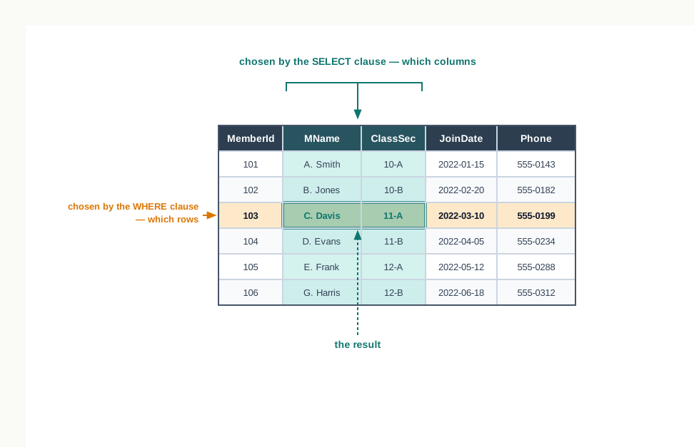
Fig. 9.9 – Filtering by SELECT and WHERE clauses.
Where every column is wanted, an asterisk stands for the whole list:
SELECT * FROM BOOK;The result is Table 9.12 exactly as it was printed — all five attributes, all eight rows. It is not reprinted here, and that is the point: SELECT * returns the table as it stands, which makes it useful for looking at a small table but wasteful, and unclear, for anything else.
9.6.2 Choosing the Columns to Retrieve
Naming columns narrows the answer to what was actually asked for. The librarian who wants a membership list does not want phone numbers on it:
SELECT MemberId, MName
FROM MEMBER;There is no WHERE clause, so every row qualifies. The columns appear in the order you named them, which need not be the order they occupy in the table.
A SELECT clause is not restricted to plain column names. It may hold an expression built from them, worked out afresh for each row. The library’s stock is worth the price of a title multiplied by the number of copies held:
SELECT Title, Price*Copies
FROM BOOK;Nothing has been added to the BOOK table. There is no stored column of stock values; the figures were calculated as the answer was assembled and will be calculated again, from whatever the prices and copy counts are, the next time the query is run. That is exactly what you want — a stored total would start drifting out of step the moment a price changed.
The heading of the second column is a small nuisance. MySQL, having no name to use, has printed the expression itself.
9.6.3 Renaming a Column with an Alias
A column in the result can be given a name of your choosing, called an alias, using the keyword AS:
SELECT Title AS Book, Price*Copies AS 'Stock Value'
FROM BOOK
WHERE Copies > 2;An alias made of a single word may be written bare, as Book is. An alias containing a space must be enclosed in quotes, as 'Stock Value' is — otherwise SQL reads the two words as two separate things and the statement fails.
The alias lives only for the duration of the query. It changes the heading on the answer and nothing else: BOOK still has a column called Title, and there is still no column called Stock Value anywhere in the database. AS may even be left out — Title Book means the same as Title AS Book — though writing it is clearer, and clarity is worth two extra letters.
9.6.4 Eliminating Repetition with DISTINCT
Some columns repeat by their nature. Several books share a category, and a query asking for categories will return that column as it stands, duplicates and all. To ask instead which categories exist, put DISTINCT after SELECT:
SELECT DISTINCT Category
FROM BOOK;Five rows come back from eight. Science appeared three times in Table 9.12 and Fiction twice, and each is now shown once. So is NULL: for the purposes of DISTINCT, all the nulls in a column count as one value, and the row for B107, whose category has not yet been decided, is represented by that single NULL.
Do not read anything into the order of Table 9.18. Without an explicit instruction, the order in which rows come back is the database’s business, not yours, and it may differ from one run to the next. Section 9.6.7 shows how to ask for an order and get it.
9.6.5 Selecting Rows with the WHERE Clause
The WHERE clause is where most of the thinking in a query goes. It holds a condition, and the condition is applied to each row separately: the row appears in the answer if the condition is true for it, and does not if it is not.
Conditions are built with the relational operators =, <, <=, >, >= and != (which may also be written <>, and means “is not equal to”).
SELECT Title, Price
FROM BOOK
WHERE Price > 300;Text is compared in the same way, with the value written in quotes. One caution belongs here: whether 'science' matches 'Science' depends on the collation chosen for the column, and with the collation MySQL uses by default it does — text comparison ignores the difference between capital and small letters. Since that is a property of the column rather than of SQL, it is safer to write the value in the case it is stored in than to rely on the comparison being forgiving.
Combining conditions
Conditions are joined with the logical operators AND, OR and NOT. AND requires both conditions to hold; OR requires at least one; NOT reverses the condition that follows it.
SELECT BookId, Title, Price
FROM BOOK
WHERE Category = 'Science' AND Price < 400;Everyday Chemistry is a science title but costs 460, so it fails the second condition and is excluded. Had the two conditions been joined by OR instead, it would have appeared, and so would every book under 400 whatever its category. The difference between AND and OR is not a detail of grammar; it is the difference between two different questions.
SELECT BookId, Category
FROM BOOK
WHERE NOT Category = 'Science';Count the rows against Table 9.12 and something is missing. There are eight books, three of them science, so five are “not science” if B107 — whose category is unknown — is counted among them. It is not. Section 9.6.8 explains why, and the reason is more interesting than a quirk.
9.6.6 Ranges and Sets: BETWEEN and IN
Two conditions come up so often that SQL provides a shorter way of writing each.
A test that a value lies within a range would ordinarily need two comparisons joined by AND. The BETWEEN operator states it once, and both limits are included:
SELECT Title, Price
FROM BOOK
WHERE Price BETWEEN 250 AND 460;Writing WHERE Price >= 250 AND Price <= 460 would give exactly the same five rows. That the boundary values are included is the detail most often got wrong, and the two books priced at 250 and the book priced at 460 are all present precisely to make it visible.
A test that a value is one of a listed set would ordinarily need several comparisons joined by OR. The membership operator IN states the set once. These two queries are equivalent:
SELECT BookId, Title, Category
FROM BOOK
WHERE Category = 'Fiction' OR Category = 'Puzzles';
SELECT BookId, Title, Category
FROM BOOK
WHERE Category IN ('Fiction', 'Puzzles');Putting NOT before IN asks for everything outside the set:
SELECT BookId, Title, Category
FROM BOOK
WHERE Category NOT IN ('Fiction', 'Puzzles');B107 is absent again, for the same unexplained reason.
9.6.7 Ordering the Result with ORDER BY
The rows of a relation have no order, so a result has no order either unless one is asked for. The ORDER BY clause asks for it, and it is written last.
Ordering by a numeric column arranges by size, and DESC reverses it. Where two rows tie, a second attribute decides between them:
SELECT Title, Price
FROM BOOK
ORDER BY Price DESC, Title;Look carefully at the two books priced at 250. DESC applies only to Price, the attribute it is written after; Title has no keyword of its own and is therefore ascending. So the prices run downwards while the tied titles run upwards, Sound and Silence before The Long Monsoon. Without the second attribute, which of those two rows came first would be unpredictable — and unpredictable is not the same as random, which makes it worse: a query may return them in the same order every day for a year and then change.
9.6.8 Handling NULL Values
Two results in this section have been short by one row. It is time to say why.
A null is not a value. It is the recorded absence of one, and SQL treats it accordingly: any comparison involving a null gives neither true nor false but a third outcome, unknown. And a row appears in an answer only when the WHERE condition is true for it — unknown is not true, so the row stays out.
That single rule explains everything. For B107, Category = 'Science' is unknown, so NOT Category = 'Science' is also unknown — negating an unknown leaves it unknown — and the row was excluded from Table 9.21 and from Table 9.24. The database is not being unhelpful. It genuinely does not know whether that book is a science book, and it declines to guess in either direction.
Since = NULL can never be true, SQL provides a separate test. IS NULL is true when the value is absent, and IS NOT NULL when it is present.
SELECT BookId, MemberId, IssueDate
FROM ISSUE
WHERE ReturnDate IS NULL;This is the query a librarian actually runs — which books are still out? — and it works only because the absence of a return date was recorded as a null rather than as some invented date.
SELECT BookId, MemberId, Fine
FROM ISSUE
WHERE Fine IS NOT NULL;9.6.9 Substring Pattern Matching with LIKE
Sometimes the exact value is not known, or is not what you are looking for. You want the titles that begin with a particular letter, or the members of a particular class whatever the section, or the books with a word somewhere in the title. The = operator is no use here, because it tests for an exact match and nothing else.
The LIKE operator compares a value against a pattern. A pattern is ordinary text in which two wild card characters stand for something other than themselves:
%stands for any run of characters, including none at all._stands for exactly one character.
SELECT BookId, Title
FROM BOOK
WHERE Title LIKE 'A%';The pattern 'A%' means “an A, then anything”. Atlas of Indian Rivers matches because the A is followed by characters, and A Short History of Maps matches because a space is a character like any other. Note the order of the two rows: nothing was asked about order, so the rows arrive in the order the table was scanned, not alphabetically.
The underscore is the stricter of the two, and that is what makes it useful:
SELECT MemberId, MName, ClassSec
FROM MEMBER
WHERE ClassSec LIKE '12_';'12_' matches a value of exactly three characters beginning with 12. Had the pattern been '12%', a value like 12 alone or 12AB would have matched too. And Vikram Das, whose ClassSec is null, matches neither pattern — a null cannot be compared, and LIKE is a comparison.
Fig. 9.10 shows the two patterns tested against the same values.
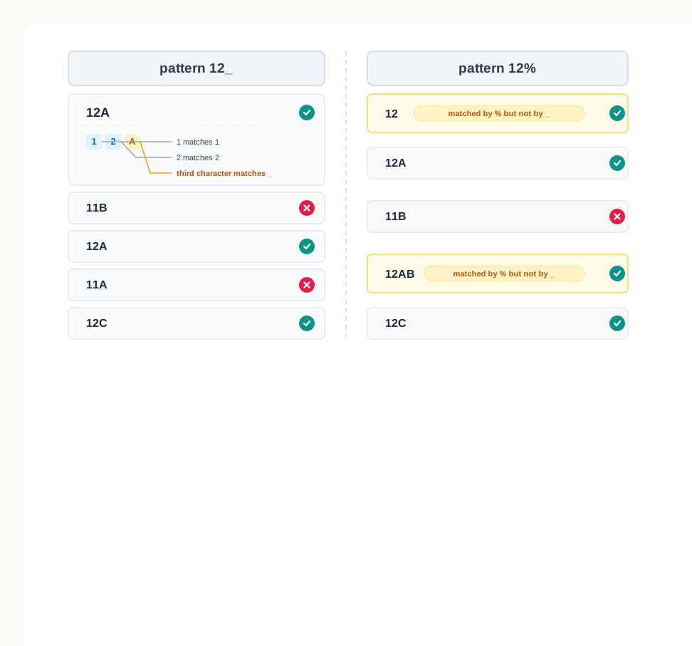
Fig. 9.10 – Pattern matching with LIKE operators.
Table 9.33 collects the patterns worth recognising at sight.
Two cautions. First, LIKE compares text, so the collation applies here as it did in Section 9.6.5 — under the default collation the pattern 'a%' matches the same titles as 'A%'. Second, a pattern with a leading % asks the database to look inside every value in the column, which is slow on a large table; it is the right query when it is the right question, but it is not free.
9.7 Data Updation and Deletion
Stored data goes out of date. A phone number that was unknown becomes known, a category that was undecided is decided, a price is revised, a record turns out to have been entered in error. The two statements that deal with all of this — UPDATE and DELETE — belong to the data manipulation language alongside INSERT, and they share one crucial feature with the SELECT statement of the previous section: they use a WHERE clause to decide which rows they act on.
That shared feature is the reason this section comes after Section 9.6 rather than beside Section 9.5. Everything you learnt about writing conditions applies here unchanged. What changes is the consequence of getting a condition wrong. A SELECT with a careless condition shows you the wrong rows; an UPDATE with the same careless condition changes them.
9.7.1 Data Updation
The UPDATE statement changes values in rows that already exist. It names the table, states which columns are to be given which new values, and states which rows are to be affected.
Rohit Barman’s phone number has reached the library at last, and the null recorded in Section 9.5.2 is replaced by the number. MySQL reports that one row matched the condition and one row was changed. Checking is a separate statement:
SELECT MemberId, MName, Phone
FROM MEMBER
WHERE MemberId = 4;Changing more than one column
Several columns can be given new values in one statement, separated by commas. The librarian has decided where A Short History of Maps belongs, and has revised its price at the same time:
UPDATE BOOK
SET Category = 'Reference', Price = 560
WHERE BookId = 'B107';
SELECT BookId, Title, Category, Price
FROM BOOK
WHERE BookId = 'B107';Both changes happened together, in one pass over the table. Writing two separate UPDATE statements would have reached the same end state, but this way there is no moment at which the row is half corrected.
Changing more than one row
A condition that matches several rows changes all of them. Fiction titles are being repriced by 25 rupees:
UPDATE BOOK
SET Price = Price + 25
WHERE Category = 'Fiction';
SELECT BookId, Title, Price
FROM BOOK
WHERE Category = 'Fiction';Notice what appears on the right of the equals sign. Price = Price + 25 is not an equation but an instruction: take the value the column holds in this row, add 25, and store the result back. Each row is treated on its own, so a table of a thousand differently priced books would be repriced correctly by that one statement. Fig. 9.11 shows the division of labour between the two clauses.
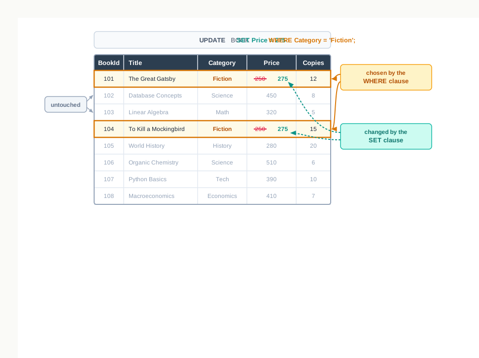
Fig. 9.11 – Updating rows in a table.
Notice also which rows were left alone. B107 is now a reference title, so it was never a candidate. Had its category still been unknown, the condition would have evaluated to unknown for that row and it would have been skipped — the rule of Section 9.6.8 applies in an UPDATE exactly as it does in a SELECT.
9.7.2 Data Deletion
The DELETE statement removes whole rows. It cannot remove part of a row — emptying one column of a row is an UPDATE that sets it to NULL, not a deletion.
That issue was recorded in error — the member changed her mind and the book never left the library — so the row goes. Because the condition names both attributes of the composite primary key, it can match at most one row, which is the safest kind of condition a DELETE can have.
SELECT BookId, IssueDate, ReturnDate
FROM ISSUE
WHERE MemberId = 3;When the database refuses to delete
Suppose Vikram Das leaves the school and the librarian tries to remove him:
DELETE FROM MEMBER
WHERE MemberId = 6;
MySQL refuses the statement, reporting that a foreign key constraint stands in the way. ISSUE holds a row recording that member 6 borrowed B106, and deleting the member would leave that row pointing at somebody who does not exist. The same protection works against an UPDATE that would change MemberId out from under the reference.
This is the foreign key of Section 9.4.4.2 doing its second job. Declaring it prevented a bad row being inserted; the same declaration now prevents a good row being stranded. If the member genuinely must go, the issue history must be dealt with first — deliberately, as a separate decision — which is exactly the pause such a decision deserves.
The last row is the one that matters in practice. After DELETE FROM ISSUE; the ISSUE table still exists, still has its five attributes and its composite key, and an INSERT will work immediately. After DROP TABLE ISSUE; the very name has gone, and the table must be created again before anything can be put into it.
Restoring the sample data
Four changes have been made in this section, and the rest of the chapter is written against the data as Tables 9.11, 9.12 and 9.13 show it. So the changes are now reversed:
UPDATE MEMBER
SET Phone = NULL
WHERE MemberId = 4;

UPDATE BOOK
SET Category = NULL, Price = 540
WHERE BookId = 'B107';

UPDATE BOOK
SET Price = 250
WHERE Category = 'Fiction';

INSERT INTO ISSUE
VALUES ('B105', 3, '2026-07-20', '2026-07-27', NULL);
That the reversal was possible at all is worth a thought. It worked only because the old values were written down in Section 9.5 before anything was changed. Nothing in the database itself remembered them, and had the changes been larger, or the record of the old values lost, no statement would have brought them back. This is the honest limitation of both statements in this section: UPDATE and DELETE do what they are told, immediately and without a copy.
9.8 Functions in SQL
A query so far has been able to show what is stored, choose among it and arrange it. What it has not been able to do is work anything out — beyond the arithmetic of Section 9.6.2, which was only addition and multiplication written out by hand.
A function in SQL is a named operation that is given one or more values and returns a value. That much is familiar from Python. What is new here is that a function in a query is applied to data held in a table, and the number of answers it produces depends on which of two kinds of function it is.
A single row function is applied to each row separately and produces one value for each row: eight rows in, eight values out. An aggregate function is applied to a whole set of rows at once and produces a single value for the set: eight rows in, one value out. Fig. 9.12 shows the difference, and it is the difference on which the rest of this section, and all of Section 9.9, depends.
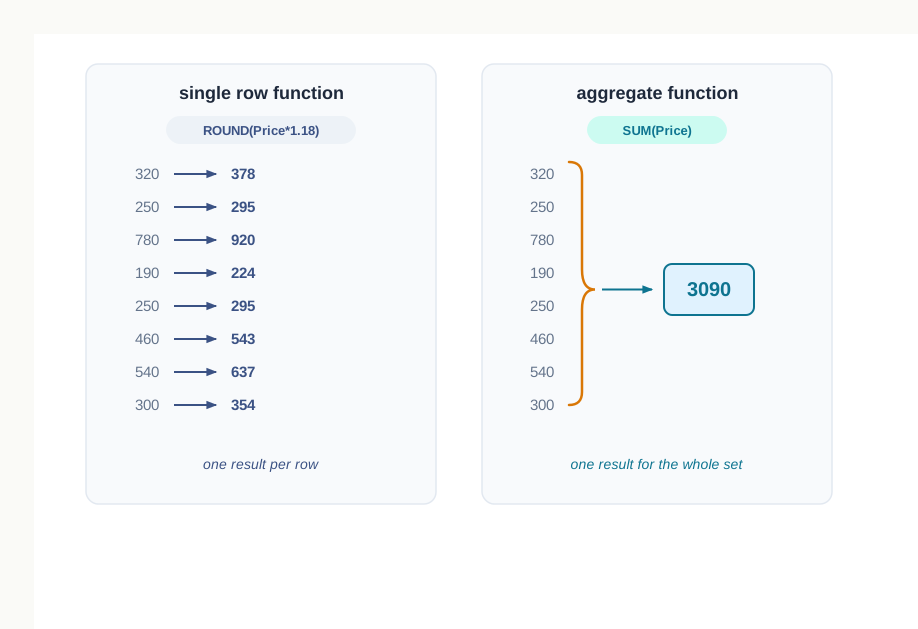
Fig. 9.12 – Single row vs aggregate functions.
9.8.1 Single Row Functions
Single row functions are also called scalar functions. Because each one produces a value from the values in a single row, it may be used anywhere a column may be used — in the SELECT clause to display something worked out, in the WHERE clause to test something worked out, and in the ORDER BY clause to arrange by something worked out.
They fall into three groups by the kind of value they work on: numbers, text, and dates.
9.8.1.1 Math Functions
ROUND takes a second argument that most students forget is optional. Written with one argument it rounds to a whole number; written with two it rounds to the stated number of decimal places. The second argument may even be negative, which rounds to the left of the decimal point: ROUND(4567.891, -2) gives 4600.
Applied to a table, these functions earn their place. The library charges 18 per cent above the printed price when a lost book has to be replaced, and the amount is wanted in whole rupees:
SELECT Title, Price, ROUND(Price * 1.18) AS Replacement
FROM BOOK
WHERE Category = 'Science';The function was worked out three times, once for each qualifying row, and nothing was stored. MOD is most useful in the WHERE clause, where it tests a property of a number rather than displaying one — here, which prices are exact multiples of 100:
SELECT Title, Price
FROM BOOK
WHERE MOD(Price, 100) = 0;9.8.1.2 String Functions
String functions work on text. They change its case, measure it, cut pieces out of it and remove unwanted spaces from its edges.
Three points about the table. Positions count from 1, not from 0 — MID('Reference', 4, 3) starts at the fourth character, which is the second e. INSTR returns 0 rather than a null when the substring is absent, which makes INSTR(...) > 0 a convenient test. And the three trimming functions remove spaces only from the ends; spaces inside the text are left alone, as they must be, since they are part of the value.
Applied to the tables, a string function does to text what ROUND did to numbers:
SELECT BookId, UCASE(Category) AS Category, RIGHT(BookId, 2) AS Serial
FROM BOOK
WHERE Copies = 1;Look at the middle row. UCASE(NULL) is NULL, not an empty string and not the word “NULL” — a function given nothing to work on has nothing to return. This is the rule of Section 9.6.8 again, now applied to functions: a null passing through a function comes out the other side as a null.
Functions may also be nested, the value returned by one becoming the argument of another. To display only the first word of each member’s name, find where the space is and take everything to its left:
SELECT MName, LEFT(MName, INSTR(MName, ' ') - 1) AS 'First Name'
FROM MEMBER
WHERE ClassSec LIKE '12_';Read the inner call first. For Ananya Rao, INSTR(MName, ' ') is 7, because the space is the seventh character. Subtracting 1 gives 6, and LEFT(MName, 6) gives the six characters before the space. The subtraction is the whole trick: without it the space itself would be included.
9.8.1.3 Date and Time Functions
A date stored as a DATE value is not text. It is a value the database understands as a date, which is why it can be compared, ordered, and taken apart into its day, month and year.
NOW() is the odd one out, and the only function in this chapter whose answer changes between one run and the next. The value shown above is what came back on the day this page was written; on yours it will be different, and that is the point of it.
SELECT MName, JoinDate, YEAR(JoinDate) AS 'Year', MONTHNAME(JoinDate) AS 'Month'
FROM MEMBER
WHERE ClassSec = '12A';Date functions are as useful in a condition as in a display. Asking for the issues made in June means asking for the rows whose issue date has 6 as its month:
SELECT BookId, IssueDate, DAYNAME(IssueDate) AS 'Day'
FROM ISSUE
WHERE MONTH(IssueDate) = 6;
Note what MONTH(IssueDate) = 6 does and does not say. It selects June of any year. Since every issue in Table 9.13 is from 2026 the distinction does not show here, but on a table holding three years of records it would matter enormously, and the condition would have to test the year as well.
9.8.2 Aggregate Functions
Aggregate functions, also called multiple row functions, are the ones that answer questions about a set of rows taken together: how many, how much altogether, the largest, the smallest, the average. Whatever the number of rows going in, one value comes out.
Four of them can be asked at once, since each produces a single value and the result is a single row:
SELECT MAX(Price) AS Costliest, MIN(Price) AS Cheapest,
       SUM(Price) AS Total, AVG(Price) AS Average
FROM BOOK;The average is shown to four decimal places. MySQL does that deliberately: an average of whole numbers is rarely a whole number, and rounding it silently would lose information, so if you want it to a chosen number of places you must say so with ROUND — which is a single row function being applied to the one row an aggregate produced.
Counting, and what counts
The two forms of COUNT differ in exactly one respect, and it is the respect that matters most:
SELECT COUNT(*) AS Titles, COUNT(Category) AS Categorised,
       COUNT(DISTINCT Category) AS Kinds
FROM BOOK;Eight rows exist. Seven of them have a category, because B107 has a null there and COUNT(Category) skips it. And those seven categories are of only four kinds, because COUNT(DISTINCT Category) counts each different value once — and, being a count of a column, ignores the null altogether.
Three different questions, three different answers, from the same eight rows.
The habit of writing COUNT(*) for everything is worth resisting. How many issues are there and how many issues carried a fine are different questions, and only the second is answered by counting a column.
Aggregates ignore nulls
That skipping is not peculiar to COUNT. Every aggregate function except COUNT(*) leaves nulls out of its working, and the consequence for AVG is the one to watch:
SELECT COUNT(*) AS Issues, SUM(Fine) AS TotalFine, AVG(Fine) AS AverageFine
FROM ISSUE
WHERE MONTH(IssueDate) = 7;Five issues were made in July, and 45 rupees were collected in fines. But the average fine is reported as 45, not as 9. AVG divided the total by the number of rows that had a fine — one — and not by the number of rows in the group. Whether that is the answer you wanted depends entirely on the question. What was the average fine charged is 45. What did an issue cost on average is 9, and to get it you would have to treat the missing fines as zeros, which the database will not do for you because it does not know that a missing fine means no fine.
Notice also the WHERE clause. It did its usual work of choosing rows, and only then were the aggregates applied to what survived. That order — rows chosen first, aggregated afterwards — explains the one place an aggregate may not go.
9.9 GROUP BY Clause in SQL
An aggregate function in Section 9.8 answered a question about the whole table: what is the total, what is the largest, how many rows are there. Useful questions, but blunt ones. The librarian rarely wants the average price of every book in the library. She wants the average price of each category — one answer for science, another for fiction, another for reference.
That is a different shape of question, and it needs one more idea. Instead of applying an aggregate to all the rows at once, gather the rows into piles by the value of some column, and apply the aggregate separately to each pile. The GROUP BY clause does the gathering.
9.9.1 Grouping Rows with GROUP BY
GROUP BY names a column. Every row whose value in that column is the same falls into the same group, and the query then produces one row of output per group rather than one per row of the table.
Eight rows went in and five came out, one for each distinct category. Add the Titles column and you get eight back; add the CopiesHeld column and you get 19, which is the total number of copies the library holds. Nothing has been lost — the rows have been rearranged into piles and each pile summarised.
B107, whose category is unknown, has a group of its own. This is the one place where nulls behave unlike everything you saw in Section 9.6.8: for grouping, all the nulls in a column are treated as belonging together, exactly as they were for DISTINCT. The group means “the books whose category has not been decided”, which is a perfectly sensible pile to have.
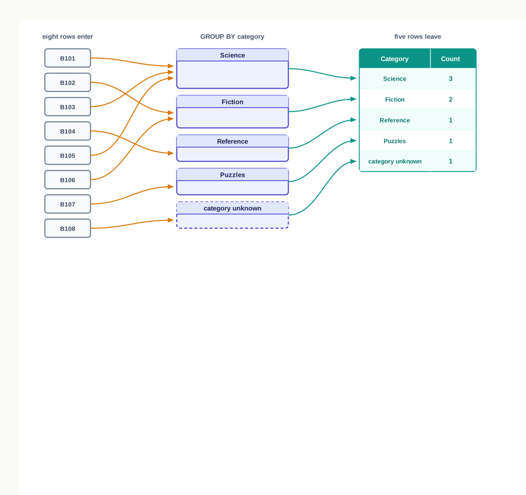
Fig. 9.13 – Grouping rows by category.
The ORDER BY clause was not decoration. GROUP BY gathers the rows but promises nothing about the order in which the finished groups come back, so a query whose output order matters has to say so. Note also where the null group lands: MySQL places nulls first when ordering upwards.
Grouping by something other than a category
Any column may be grouped by, not only one that looks like a classification. Grouping the issue register by book code answers a question the librarian asks often — which titles are actually moving:
SELECT BookId, COUNT(*) AS TimesIssued
FROM ISSUE
GROUP BY BookId
ORDER BY BookId;Six groups, from eight rows. And now look at what is not in the answer. B107 and B108 are missing, because they have never been issued and so have no rows in ISSUE to be gathered. A group can only be formed from rows that exist. If the question were “how many times has each book been issued, including those issued never”, this query could not answer it — and Section 9.11 shows the statement that can.
Choosing the rows before grouping them
WHERE and GROUP BY work together in a fixed order: the WHERE clause throws out rows first, and only the survivors are gathered.
SELECT MemberId, COUNT(*) AS Borrowings
FROM ISSUE
WHERE MONTH(IssueDate) = 7
GROUP BY MemberId
ORDER BY MemberId;Five of the eight issues were made in July, and those five gathered into four groups. Member 1, whose two borrowings were both in June, is absent altogether — not because the count for that member was zero, but because after the WHERE clause there were no rows left to form a group from. There is no group with a count of zero, in this query or in any other.
Aggregates within groups
Every aggregate function from Section 9.8 works inside a group exactly as it worked over a whole table:
SELECT Category, COUNT(*) AS Titles, ROUND(AVG(Price)) AS AveragePrice
FROM BOOK
GROUP BY Category
ORDER BY AveragePrice DESC;The science figure is worth checking by hand: 320, 460 and 300 add to 1080, and 1080 divided by 3 is 360. Notice that this arrangement is ordered by a column that does not exist in the table at all — AveragePrice is worked out by the query, and the query may then order by it.
9.9.2 Selecting Groups with HAVING
Section 9.8 ended with a statement MySQL would not accept: a WHERE clause containing an aggregate. The reason was that WHERE examines one row at a time, and at that moment no group exists for an aggregate to describe.
But the question behind that rejected statement is a real one. Which categories have more than one title? is a question about groups, not about rows, and it needs a filter that runs after the grouping rather than before it. That filter is the HAVING clause.
SELECT Category, COUNT(*) AS Titles
FROM BOOK
GROUP BY Category
HAVING COUNT(*) > 1
ORDER BY Category;The five groups of Table 9.54 were all formed as before. HAVING then examined each finished group, kept the two whose count exceeded one, and discarded the other three — including the null group, whose single title was not enough.
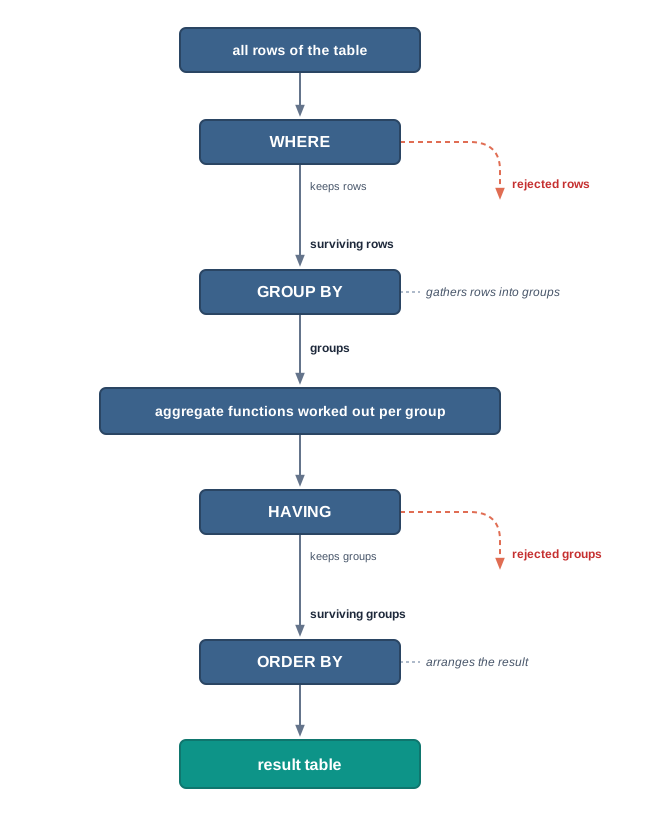
Fig. 9.14 – Execution order of SELECT statement clauses.
Fig. 9.14 is the whole of this section in one picture, and it also explains a rule of writing that would otherwise look arbitrary: the clauses must be written in the order SELECT, FROM, WHERE, GROUP BY, HAVING, ORDER BY, because that is very nearly the order in which the work is done.
All of them can appear together. This query asks which members have returned more than one book:
SELECT MemberId, COUNT(*) AS Returned
FROM ISSUE
WHERE ReturnDate IS NOT NULL
GROUP BY MemberId
HAVING COUNT(*) > 1
ORDER BY MemberId;Follow the row through the four clauses. Six of the eight issues have a return date, so WHERE keeps six rows. Those six gather into four groups — members 1, 2, 3 and 6, with counts of 2, 1, 2 and 1. HAVING keeps the two groups whose count is above one. ORDER BY arranges what is left. Change any one of the four clauses and you are asking a different question.
9.10 Operations on Relations
Every query so far has drawn on one relation. But a relation is a set of tuples, and sets can be combined: put together, overlapped, subtracted from one another. SQL inherits four such operations, and they are worth understanding both for their own sake and because the last of them is the machinery on which Section 9.11 is built.
The school library keeps two more lists besides the three tables you already know. The reading circle and the quiz club each meet on Saturday, and each keeps a record of who takes part. Both were created and filled with the statements of Sections 9.4 and 9.5, and both hold the same three attributes.
Three questions arise the moment the librarian has both lists in front of her. Who takes part in either activity? Who takes part in both? And who is in the reading circle but not in the quiz club? Those three questions are answered by the first three operations of this section, and all three carry a condition that has to be met before they can be asked at all.
Both lists here hold a membership number, a name and a class, in that order, so they are union compatible and all three operations are available.
9.10.1 Union
The union of two relations holds every tuple that appears in either of them. A tuple appearing in both is shown once, not twice — the result is a set, and a set does not hold the same member twice.
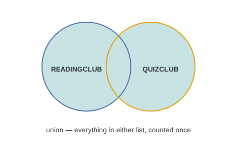
Fig. 9.15 – Union of two relations.
In SQL the operation is written by placing the keyword UNION between two SELECT statements:
SELECT * FROM READINGCLUB
UNION
SELECT * FROM QUIZCLUB
ORDER BY MemberId;Four tuples and three tuples gave five, not seven. Kavya Menon and Sneha Patil are in both lists, and each appears once in the answer — which is exactly what the librarian ordering refreshments for Saturday needs to know.
The ORDER BY clause is written once, at the very end, and arranges the finished result. It cannot be attached to either SELECT on its own, because neither of them is the answer; the answer is what the two produce together.
9.10.2 Intersect
The intersection of two relations holds only the tuples that appear in both.
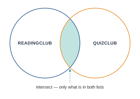
Fig. 9.16 – Intersection of two relations.
Two members out of the seven entries on the two lists are doing both things on the same Saturday afternoon, which is the sort of clash a timetable is meant to catch early.
The keyword is INTERSECT, written between two SELECT statements exactly as UNION was. It is part of the SQL standard and is available in recent versions of MySQL; older versions do not provide it, and on such a server the same question is answered with the join of Section 9.11, which matches rows of one table against rows of another.
9.10.3 Minus
The difference of two relations holds the tuples that are in the first and not in the second. It is written with a minus sign, and in some systems the keyword is MINUS while in others it is EXCEPT.
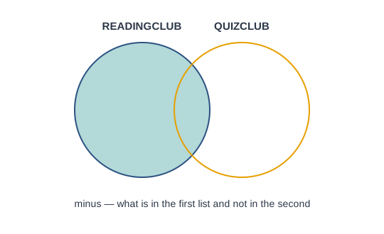
Fig. 9.17 – Difference (minus) of two relations.
Now reverse the two relations and the answer changes completely:
This is the one property of the three operations that catches students out. Union and intersect give the same answer whichever relation is written first; minus does not. A minus B and B minus A are different questions, and Fig. 9.17 makes the reason plain — reversing the operation shades the other crescent.
9.10.4 Cartesian Product
The fourth operation is different in kind. It does not compare tuples at all, and it does not require the two relations to be union compatible. It simply pairs every tuple of the first relation with every tuple of the second.
Because every tuple is paired with every tuple, the size of the result follows arithmetically from the sizes of the two relations. The degree of the product is the sum of the two degrees, since a row of the product carries all the attributes of both. The cardinality of the product is the product of the two cardinalities, since each of the first relation’s tuples contributes as many rows as the second relation has tuples.
For READINGCLUB and QUIZCLUB the two degrees are 3 and 3, so the product has degree 6. The two cardinalities are 4 and 3, so the product has cardinality \(4 \times 3 = 12\).
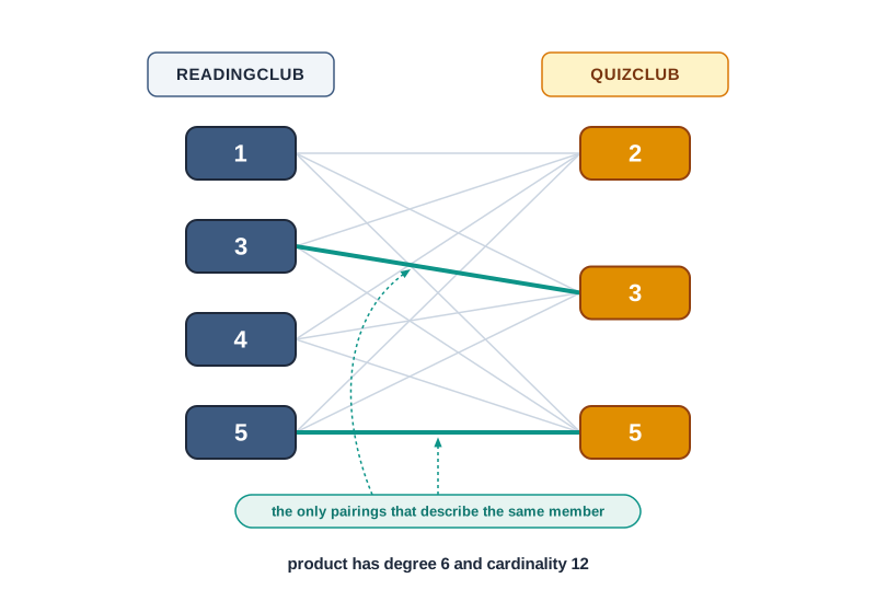
Fig. 9.18 – Cartesian product of two relations.
Read Table 9.67 honestly and most of it is nonsense. The first row places Ananya Rao’s details beside Imran Sheikh’s and asserts nothing whatever about either of them; it exists only because the operation makes every pairing, whether or not the pairing means anything. Of the twelve rows, exactly two — the fifth and the last — put a member’s details beside her own, and those are the two that Fig. 9.18 draws heavily.
That observation is the whole of the next section in advance. The cartesian product produces every possible combination; a useful answer is some small selection from it, picked out by a condition that says which combinations are meaningful. Section 9.11 shows how the condition is written, and how SQL is asked to make the product in the first place.
9.11 Using Two Relations in a Query
Section 9.1 began with a difficulty: the school office could answer a question from any one register easily, and a question that crossed two registers only by matching entries by hand. Everything since then has worked inside a single relation. This section finally crosses the boundary.
The difficulty is real in the library too. Table 9.13 records that book B106 went out to member 6 on 5 July, and there is nothing in it to say what B106 is or who member 6 is. Those facts are in BOOK and in MEMBER, exactly where they belong — a title is a fact about a book, not about a borrowing. Splitting the facts that way is good design, and the price of it is that a single useful question now needs two tables at once.
9.11.1 Cartesian Product on Two Tables
To use two tables in one query, name both in the FROM clause, separated by a comma. What comes back is the cartesian product defined in Section 9.10.4 — every row of the first table paired with every row of the second.
SELECT * FROM READINGCLUB, QUIZCLUB;The result is Table 9.67, printed in the previous section: twelve rows of degree 6, of which ten pair one member’s details with a different member’s and mean nothing at all.
Now consider the same thing done to the library’s real tables. SELECT * FROM BOOK, ISSUE; pairs each of the eight books with each of the eight issue records, giving a relation of degree 10 and cardinality 64. It is not printed here, and the reason is worth stating plainly: only 8 of those 64 rows describe a real borrowing, and the other 56 attach a title to a borrowing that was not of that title. The product is not the answer. It is the raw material from which the answer is selected.
Selecting from it is done with an ordinary WHERE clause:
SELECT * FROM READINGCLUB R, QUIZCLUB Q
WHERE R.MemberId = Q.MemberId
ORDER BY R.MemberId;Two rows survive out of twelve, and they are precisely the two lines drawn heavily in Fig. 9.18-4. The query has answered the intersection question of Section 9.10.2 without using INTERSECT at all.
Naming the tables and their columns
Two things in that statement are new. R and Q are table aliases, short names given to the tables in the FROM clause so that they can be referred to briefly afterwards. And R.MemberId is a qualified attribute name — the table, then a full stop, then the attribute.
The qualification is not optional here. Both tables have an attribute called MemberId, so writing WHERE MemberId = MemberId would leave MySQL with no way of knowing which MemberId was meant, and it rejects the statement as ambiguous. Wherever an attribute name occurs in more than one of the tables named in FROM, every mention of it must say which table it comes from.
A table alias holds only for the query it is written in. Nothing in the database is renamed, and the next query may use different aliases or none. One rule goes with it: once a table has been given an alias in the FROM clause, the original name can no longer be used in that query. Having written QUIZCLUB Q, you must write Q.MName, not QUIZCLUB.MName.
9.11.2 Join on Two Tables
A join combines rows from two tables on a stated condition, keeping only the combinations that satisfy it. What Section 9.11.1 did by hand — make every pairing, then throw most of them away — is what a join does, and SQL provides a way of saying so directly.
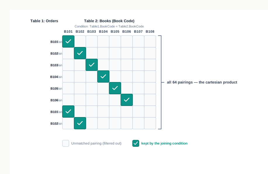
Fig. 9.19 – Filtering a cartesian product with a joining condition.
The condition is almost always the equality of a primary key in one table with a foreign key in the other, because that equality is exactly what “these two rows describe the same thing” means. Here it is written in the WHERE clause, as in the previous subsection:
SELECT B.Title, I.MemberId, I.IssueDate
FROM BOOK B, ISSUE I
WHERE B.BookId = I.BookId
ORDER BY B.BookId, I.IssueDate;Eight rows — one for each row of ISSUE, which is what you should expect. Every issue names exactly one book, so every issue row finds exactly one partner in BOOK. And A Short History of Maps and Weather and Wind do not appear anywhere in the answer, because they have never been issued and so have no partner to be joined to. The two empty columns in Fig. 9.19 are those two books.
The JOIN clause
The same join may be written with the condition inside the FROM clause, using the keyword JOIN and the keyword ON. This is the form that says most plainly what is happening, because the joining condition sits beside the tables it joins rather than among the conditions that select rows.
Rohit Barman is missing, and for the same reason two books were missing from Table 9.70: he has borrowed nothing, so there is no row in ISSUE for his row of MEMBER to be joined to. A join shows what matched. It says nothing about what did not.
Selecting and grouping across a join
Once two tables are joined, the result behaves like any other relation, and every clause of the previous sections applies to it unchanged. A WHERE clause narrows the rows:
SELECT M.MName, I.BookId, I.IssueDate
FROM MEMBER M JOIN ISSUE I
ON M.MemberId = I.MemberId
WHERE I.ReturnDate IS NULL
ORDER BY I.IssueDate;This is the query the library actually needs — Table 9.29 found the outstanding issues but could only give their book codes, and it is a name, not a code, that lets the librarian send a reminder.
Grouping works across a join too, and this is where the chapter’s ideas come together. Which kinds of book are borrowed most?
SELECT B.Category, COUNT(*) AS TimesIssued
FROM BOOK B JOIN ISSUE I
ON B.BookId = I.BookId
GROUP BY B.Category
ORDER BY TimesIssued DESC, B.Category;Follow the work through. The join produced the eight rows of Table 9.70, each now carrying its book’s category as well. Those eight gathered into four groups, and the counts are what the librarian would use when deciding what to buy next. The category NULL does not appear, because the only uncategorised book has never been issued and so contributed no row to the join.
9.11.3 Natural Join
Look again at what the joining condition does. It keeps the pairs of rows in which BOOK.BookId and ISSUE.BookId hold the same value — so in every row of the result, those two columns are identical. Showing both is showing the same fact twice.
A natural join removes that redundancy. It joins two tables on their commonly named attributes, using equality, and shows each such attribute only once.
SELECT BookId, Title, MemberId, IssueDate
FROM BOOK NATURAL JOIN ISSUE
ORDER BY BookId, IssueDate;The rows are the same eight as before. Two things about the statement are different: no joining condition was written, and BookId needed no qualifier. Both follow from the same fact — there is only one BookId column in the result, so there is nothing to be ambiguous about.
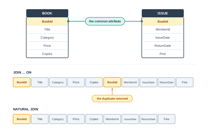
Fig. 9.20 – Natural join removing duplicate columns.
The convenience carries a real risk, and it is worth knowing before you rely on it. A natural join uses every attribute the two tables have in common, whether or not you intended it. BOOK and ISSUE share only BookId, so the join is the one you want. But if ISSUE had also carried a column called Category — meaning the category of the borrower, say — the natural join would silently have required both the book codes and the two categories to match, and would have returned a handful of rows or none at all, with no error to warn you.
Whichever form is used, one arithmetic fact holds. Joining two tables on an equality condition takes one join; three tables take two; in general, \(N\) tables joined on equality need \(N-1\) joins, because each join brings in one further table. This chapter stops at two, which is enough for every question the library has asked.
9.12 Summary
Why a query language exists
Data held in ordinary files can only be reached by a program that knows where the data is, in what order it is stored and how to walk through it. That knowledge sits inside every such program, and changing the storage means changing them all.
In the relational data model all data is held in relations — tables of rows and columns. A row is a tuple, a column is an attribute, no two tuples of a relation are identical, and the order in which tuples and attributes appear carries no meaning.
The degree of a relation is the number of its attributes; the cardinality is the number of its tuples. Degree changes only when the design changes; cardinality changes whenever a row is added or removed.
A primary key is the attribute, or combination of attributes, that identifies each tuple uniquely. Its values may neither repeat nor be null, and a relation has at most one. A foreign key is an attribute of one relation whose value must match the primary key of another, and it is what allows a question to travel between two tables.
A query is a request that states the data wanted, not the steps for finding it. A query language is the language such requests are written in, and the database management system decides how the request is to be satisfied.
The language itself
Structured query language is the standard language of relational systems. It defines the structure of data, declares constraints on it, stores and modifies it, and retrieves it.
Keywords and column names are not case-sensitive. Database and table names may or may not be, depending on the operating system, so a name should always be written in the case in which it was created.
Every statement ends with a semicolon. Pressing Enter before the semicolon changes the prompt to
->and continues the same statement on the next line, which is how a long statement is spread over several lines.Every query returns a table, whatever the question was.
Data types and constraints
The data type of an attribute fixes both the values it may hold and the operations that may be performed on them. The commonly used types are
CHAR(n),VARCHAR(n),INT,FLOATandDATE.CHAR(n)is fixed length: every value occupies space forncharacters and shorter values are padded with spaces.VARCHAR(n)is variable length: only the characters stored occupy space. Fixed-length codes suitCHAR; names and addresses suitVARCHAR.A number made only of digits is not always a numeric value. A phone number or an identifier is compared and displayed but never calculated with, so it is stored as text — which also keeps its leading zeros and avoids the limits of
INT.A constraint is a rule declared on an attribute and enforced by the database on every insertion and update. The commonly used constraints are
NOT NULL,UNIQUE,DEFAULT,PRIMARY KEYandFOREIGN KEY.A null value is the recorded absence of a value — not zero, and not empty text. Unless a constraint forbids it, any attribute may hold a null, and a
UNIQUEattribute may hold several.
Defining the structure
The data definition language creates, changes and removes structure. A database is made with
CREATE DATABASEand selected withUSE; its tables are listed bySHOW TABLESand made withCREATE TABLE, which names each attribute with its data type and any constraints.DESCRIBE, orDESC, reports the structure of a table: each attribute, its type, whether it may be null, its part in any key and its default value.ALTER TABLEchanges an existing structure. It can add a primary key or a foreign key, add aUNIQUEorDEFAULTconstraint, add or drop an attribute, modify an attribute’s data type or constraints, and drop the primary key.A primary key built from two or more attributes is a composite primary key. It guarantees that no two tuples agree on the whole combination, while each attribute on its own may repeat freely.
Before a foreign key can be declared, the referenced table must already exist, the referenced attribute must be the primary key of that table or part of it, and the two attributes must have the same data type and size.
MODIFYreplaces an attribute’s definition rather than adjusting it, so the data type must be restated every time and any constraint not repeated is lost.DROP TABLEandDROP DATABASEremove the structure and all the data in it, permanently. A table cannot be dropped, and its primary key cannot be removed, while another table’s foreign key refers to it.
Putting data in, changing it and taking it out
The data manipulation language works on the rows:
INSERT,SELECT,UPDATEandDELETE.Tables that refer to no other table must be filled first, and a table carrying foreign keys only after every table it refers to has been filled.
INSERT INTOhas two forms. Without a column list, a value must be given for every attribute, in the order the attributes were declared. With a column list, only the named attributes are supplied, and each attribute left out takes its default value or a null.A declared default is used only when an attribute is omitted. Writing
NULLin its place stores a null instead.UPDATEchanges values in existing rows, with aSETclause naming the attributes and their new values.DELETEremoves whole rows. In both, theWHEREclause decides which rows are affected, and omitting it affects every row in the table.DELETEempties rows but leaves the table, its attributes, its keys and its constraints in place.DROPremoves the table itself. A foreign key refuses a deletion that would leave a reference pointing at nothing.
Asking questions of one table
A
SELECTstatement makes two independent choices: theSELECTclause chooses the columns, and the optionalWHEREclause chooses the rows.SELECT *asks for every column.The
SELECTclause may hold an expression worked out for each row. Nothing is stored; the value is calculated afresh each time the query runs.An alias, written with
AS, renames a column in the result. It lasts only for that query, and an alias containing a space must be quoted.DISTINCTremoves repeated values from the result, treating all nulls in a column as one value.Conditions are built with the relational operators
=,<,<=,>,>=and!=, and combined with the logical operatorsAND,ORandNOT.BETWEENtests whether a value falls within a range, and both limits are included.INtests whether a value is one of a listed set, andNOT INasks for everything outside it.ORDER BYarranges the result.ASCis ascending and is what happens if nothing is written;DESCis descending and applies only to the attribute it follows. A second attribute settles rows that tie on the first. WithoutORDER BY, the order of the rows is not promised.Any comparison involving a null gives neither true nor false but unknown, and a row appears in an answer only when its condition is true. So a row with a null is excluded by a condition and by its negation alike. A null is tested for with
IS NULLandIS NOT NULL, never with=.LIKEcompares a value against a pattern built with two wild card characters:%stands for any run of characters including none, and_stands for exactly one character.
Functions
A single row function is applied to each row separately and returns one value per row. An aggregate function is applied to a set of rows and returns one value for the whole set.
The math functions are
POWER(),ROUND()andMOD().ROUND()takes an optional second argument giving the number of decimal places.The string functions are
UCASE(),LCASE(),MID(),LENGTH(),LEFT(),RIGHT(),INSTR(),LTRIM(),RTRIM()andTRIM(). Character positions are counted from 1, and the trimming functions remove spaces only from the ends of a string.The date and time functions are
NOW(),DATE(),MONTH(),MONTHNAME(),YEAR(),DAY()andDAYNAME(). They may be used to display part of a date or to test it in a condition.A null passing through a single row function comes out as a null.
The aggregate functions are
MAX(),MIN(),AVG(),SUM()andCOUNT(). All of them exceptCOUNT(*)leave nulls out of their working, so an average is divided by the number of values present, not by the number of rows.COUNT(*)counts rows;COUNT(column)counts the rows in which that column is not null. They answer different questions and can give different numbers from the same table.An aggregate cannot appear in a
WHEREclause, because that clause examines one row at a time and no group yet exists for the aggregate to describe.
Grouping
GROUP BYgathers rows into groups by the value of an attribute and produces one row of output per group. All the nulls in that attribute form a single group.WHEREacts before the gathering and decides which rows take part;HAVINGacts after it and decides which finished groups are shown. OnlyHAVINGmay test the value of an aggregate.Every attribute in the
SELECTclause of a grouped query must either be the attribute grouped by or sit inside an aggregate function.A group is formed only from rows that exist, so no group ever has a count of zero.
The clauses are written in the order
SELECT,FROM,WHERE,GROUP BY,HAVING,ORDER BY, which is very nearly the order in which the work is done.
Operations on relations
Union, intersect and minus may be applied only to relations that are union compatible — the same number of attributes, with corresponding attributes drawn from the same domain.
Union holds every tuple in either relation, each appearing once. Intersect holds the tuples in both. Minus holds the tuples in the first that are not in the second, and unlike the other two it gives a different answer if the relations are reversed.
The cartesian product pairs every tuple of one relation with every tuple of the other. It needs no compatibility. Its degree is the sum of the two degrees, and its cardinality is the product of the two cardinalities.
Using two relations in a query
Naming two tables in the
FROMclause gives their cartesian product, most of whose rows are meaningless pairings. A condition of equality then keeps only the pairs of rows that describe the same thing.A table alias is a short name given to a table for the duration of one query. Where an attribute name occurs in more than one of the tables named, every mention of it must be qualified with the table it comes from.
A join combines rows of two tables on a stated condition. The condition is almost always a primary key in one table set equal to a foreign key in the other, and it may be written either in the
WHEREclause or in theFROMclause withJOINandON.A join shows only what matched. A row with no partner in the other table — a book never issued, a member who never borrowed — does not appear in the result at all.
A natural join joins two tables on every attribute whose name they share, using equality, and shows each such attribute once instead of twice. Its convenience is also its risk, since an unintended shared name would silently be joined on as well.
Joining \(N\) tables on equality conditions requires \(N-1\) joins.
9.13 Key Terms
Aggregate function — a function applied to a whole set of rows at once, returning a single value for the set;
MAX(),MIN(),AVG(),SUM()andCOUNT().Alias — a name given to a column of a result, using
AS, for the duration of one query only.Attribute — a named column of a relation, holding one kind of fact about every tuple in it.
Cardinality — the number of tuples in a relation.
Clause — a part of an SQL statement introduced by a keyword, such as
FROM,WHEREorORDER BY, each answering one question about the request.Composite primary key — a primary key built from two or more attributes together, so that no two tuples agree on the whole combination although each attribute may repeat on its own.
Constraint — a rule declared on an attribute and enforced by the database on every insertion and update;
NOT NULL,UNIQUE,DEFAULT,PRIMARY KEYandFOREIGN KEY.Data definition language (DDL) — the SQL statements that create, change and remove structure, such as
CREATE,ALTERandDROP.Data manipulation language (DML) — the SQL statements that work on the rows held in tables:
INSERT,SELECT,UPDATEandDELETE.Data type — the declaration of what kind of value an attribute may hold, which also fixes the operations that may be performed on it.
Database — an organised collection of related data, held so that it can be retrieved and updated as required.
DDL — data definition language.
Degree — the number of attributes in a relation.
DML — data manipulation language.
Foreign key — an attribute of one relation whose value must match a value of the primary key of another relation.
Function — a named operation that is given one or more values and returns a value.
Join — an operation that combines each tuple of one relation with those tuples of another that satisfy a stated condition.
Natural join — a join made on every attribute whose name the two tables share, using equality, in which each such attribute appears once in the result rather than twice.
Null value — the recorded absence of a value, written
NULL; not zero and not empty text.Open source — software whose source code is published and which may be downloaded and used free of cost.
Primary key — the attribute, or combination of attributes, that identifies each tuple of a relation uniquely; its values may neither repeat nor be null, and a relation has at most one.
Query — a request made to a database that states the data wanted rather than the steps for finding it.
Query language — the language in which queries are written, through which a user defines, stores, modifies and retrieves the data held in a database.
RDBMS — relational database management system.
Referenced table — the table whose primary key a foreign key points at.
Referencing table — the table that holds the foreign key.
Relation — a table with a fixed set of named columns and any number of rows, in which no two rows are identical and the order of rows and columns carries no meaning.
Relational data model — the model in which all data is held in relations, each row a tuple and each column an attribute drawn from a single domain.
Relational database management system (RDBMS) — software that stores data as relations, enforces the rules declared on them and answers queries put to them.
Schema — the description of a relation’s structure: its name, its attributes, their data types and the constraints on them.
Single row function — a function applied to each row separately, returning one value for every row; also called a scalar function.
SQL — structured query language.
Structured query language (SQL) — the standard language of relational database management systems, used to define the structure of data, declare constraints on it, store and modify it, and retrieve it.
Table alias — a short name given to a table in the
FROMclause of a query, used to qualify attribute names for the duration of that query.Tuple — a row of a relation, holding the facts about one thing.
Wild card character — a character in a
LIKEpattern that stands for something other than itself:%for any run of characters including none, and_for exactly one character.
9.14 Points to Ponder
A query says what is wanted and leaves the method to the database. That is convenient — but it also means you cannot tell, from the statement alone, whether an answer will arrive in a moment or in an hour. Is a language that hides its own cost a good language to build on?
A null is not zero, and the chapter treated that distinction as an obvious gain. Yet it forces three outcomes on every comparison instead of two, and lets a condition and its negation both reject the same row. Would a system that simply forbade missing values be easier to reason about, and what would it cost the people entering the data?
Constraints refuse work. A foreign key stops a row being inserted, a primary key stops a duplicate, a
NOT NULLstops an incomplete record. Every one of them makes the database harder to use in the moment. Why is that a reasonable price, and is there a point at which a table can be over-constrained?The library’s design puts a title in one table and a borrowing in another, so that almost every useful question needs a join. Keeping the title in the issue register would make those questions unnecessary. What exactly would go wrong, and is the answer the same for a library with fifty books as for one with fifty thousand?
UPDATEandDELETEwill change every row in a table if theWHEREclause is left out, and no warning is given. The designers of SQL could have made the clause compulsory. Why might they have chosen not to, and where should the protection against a careless statement actually live?A natural join works out for itself which attributes to join on, from the names the two tables happen to share. Is inferring an operation from a naming coincidence ever a sound idea, or is the convenience of it a trap dressed as a shortcut?
9.15 Objective Questions
Which constraint ensures that no two rows hold the same value in a column, while still permitting more than one row to hold a null in it? [1 mark]
NOT NULLUNIQUEPRIMARY KEYDEFAULT
Relation P has degree 3 and cardinality 5. Relation Q has degree 4 and cardinality 2. The cartesian product P X Q has: [1 mark]
- degree 7 and cardinality 7
- degree 7 and cardinality 10
- degree 12 and cardinality 10
- degree 3 and cardinality 10
Which clause is used to place a condition on the value of an aggregate function? [1 mark]
WHEREGROUP BYHAVINGORDER BY
A table has 10 rows, of which 3 hold a null in the column
Bonus. The querySELECT COUNT(*), COUNT(Bonus) FROM PAYROLL;returns: [1 mark]- 10 and 10
- 10 and 7
- 7 and 7
- 7 and 10
Fill in the blank: a null value in a column can be tested only with the ______ operator, never with the equals sign. [1 mark]
Fill in the blank: in a
LIKEpattern, the ______ character stands for exactly one character. [1 mark]State whether true or false: the
DELETEstatement removes the rows of a table and also the structure of the table. [1 mark]State whether true or false: a declared
DEFAULTvalue is used when a column is left out of the column list of anINSERT INTOstatement, but not whenNULLis written for it. [1 mark]Write the output of the statement
SELECT LENGTH(TRIM(' Jaipur '));[1 mark]Write the full form of each of these abbreviations: DDL, DML, RDBMS, SQL. [1 mark]
Match each function in the first list with what it returns, from the second list. [1 mark]
| Column A | Column B |
|---|---|
a. INSTR(string, substring) |
i. the remainder after a division |
b. MOD(a, b) |
ii. the last n characters of a string |
c. DAYNAME(date) |
iii. the position at which a substring first occurs |
d. RIGHT(string, n) |
iv. the name of the weekday |
- Assertion (A): A foreign key column may hold a null value. Reason (R): A null in a foreign key means the row is not yet linked to any row of the referenced table, which is a legitimate state. [1 mark]
- Both A and R are true, and R is the correct explanation of A.
- Both A and R are true, but R is not the correct explanation of A.
- A is true but R is false.
- A is false but R is true.
- Assertion (A): The queries
SELECT * FROM BOOK WHERE NOT Price > 300;andSELECT * FROM BOOK WHERE Price <= 300;always return the same rows. Reason (R): A comparison involving a null gives unknown, and a row is returned only when its condition is true. [1 mark]- Both A and R are true, and R is the correct explanation of A.
- Both A and R are true, but R is not the correct explanation of A.
- A is true but R is false.
- A is false but R is true.
9.16 Check Your Concepts
Several questions in this block, and all of those in the next, refer to the table in Table 9.76, which records the stock held at a school stationery counter. ItemCode is the primary key, UnitPrice and Stock are of type INT, and PurchaseDate is of type DATE.
Define the degree and the cardinality of a relation, and state both for the table in Table 9.76. [2 marks]
A null value is not the same as zero. Explain the difference, and give one example of a column in which storing zero in place of a null would give a misleading answer to a later query. [2 marks]
Give two points of difference between
CHAR(n)andVARCHAR(n). [2 marks]A school stores a ten-digit contact number in a column declared as
INT. State two things that go wrong, and give the data type that should have been used. [2 marks]Differentiate between the
DELETEstatement and theDROP TABLEstatement, in two points. [2 marks]Write a single query on the table in Table 9.76 to display the item name and unit price of all items in the
Papercategory, dearest first. [2 marks]Differentiate between the
WHEREclause and theHAVINGclause, giving one query on the table in Table 9.76 to illustrate each. [3 marks]Write three queries on the table in Table 9.76: (i) to display each category once; (ii) to display the item name and purchase date of all items purchased in January 2026; (iii) to display each category with the total stock held in it. [3 marks]
Explain what a foreign key is, and state the three conditions that must hold before a foreign key can be declared on a column. [3 marks]
Write four statements for the table in Table 9.76: (i) to add a column
Supplierof typeVARCHAR(20); (ii) to increase the unit price of every item in theColourcategory by 10 per cent; (iii) to display the item names longer than ten characters; (iv) to display the number of items for which no stock figure has been recorded. [4 marks]The
MODIFYoption ofALTER TABLErequires the data type of a column to be written again even when the type is not being changed. Explain why, and describe what is silently lost when this is forgotten. [4 marks]A school wants to record, for each period of the timetable, the class, the day of the week and the teacher on duty. No single column identifies one record uniquely. Explain how you would design the primary key of this table, state which columns it would use, and give one row that a badly chosen key would wrongly allow. [5 marks]
Compare the cartesian product of two tables, a join with an
ONcondition, and a natural join. Your answer should cover how the rows to be combined are decided in each case, how many columns the result carries, and one situation in which the natural join would give a result the writer of the query did not intend. [5 marks]
9.17 Output & Debugging
All the questions in this block refer to the table in Table 9.76.
- Give the result of the following query, with the rows in the order in which they would appear. [2 marks]
SELECT ItemName, UnitPrice
FROM STATIONERY
WHERE UnitPrice BETWEEN 35 AND 90
ORDER BY UnitPrice DESC;- Give the values returned by the following query, and explain in one sentence why the first two are different. [3 marks]
SELECT COUNT(*), COUNT(Stock), SUM(Stock)
FROM STATIONERY;- State how many rows the following query returns, and what each row contains. [2 marks]
SELECT Category, COUNT(*)
FROM STATIONERY
GROUP BY Category
HAVING COUNT(*) > 1;- The following query was written to list the items for which no stock figure has been recorded. It runs without any error message and returns an empty set. Identify the mistake and rewrite the query correctly. [2 marks]
SELECT ItemCode, ItemName
FROM STATIONERY
WHERE Stock = NULL;- The following query is rejected by MySQL. Identify the single mistake in it, explain in one sentence why the query cannot be answered as written, and rewrite it so that it runs. [3 marks]
SELECT ItemName, Category, COUNT(*)
FROM STATIONERY
GROUP BY Category;- A student intended to correct the price of one item and typed the statement below. State exactly what the statement does to the table in Table 9.76, and rewrite it so that it does what was intended for the item
S04. [2 marks]
UPDATE STATIONERY
SET UnitPrice = 160;
9.18 Case-Based Questions
- A school records its annual sports meet in two tables.
EventIdis the primary key of EVENT,EntryNois the primary key of ENTRY, andEventIdin ENTRY refers to EVENT. A null inPointsmeans the event has not yet been judged. [5 marks]
a. Name the referencing table and the referenced table, and state what the database would do if an entry were inserted for the event `E09`. [1 mark]
b. Write a query using both tables to display the event name, house name and points for every entry in an event held on `2026-09-14`. [2 marks]
c. Write a query to display each house with the total points it has scored, the highest total first, and state which of the two tables the `Points` column comes from. [2 marks]- A small shop keeps its stock in the table below. The table was created with data types but with no constraints at all, and the state it has reached is the result. [5 marks]
a. Two separate problems can be seen in Table 9.79. Describe each, and name the constraint that would have prevented it. [2 marks]
b. Write the statement that would make `PCode` the primary key of this table, and explain why it would be refused on the data as it stands. [2 marks]
c. The shop also keeps a SUPPLIER table whose primary key is `SupCode`, and it holds rows for `SUP1` and `SUP2` only. State what would happen if `SupplierCode` were now declared a foreign key referring to it. [1 mark]
9.19 Programming Practice
A science laboratory wants a database of its equipment. Each item has a code of exactly five characters that identifies it; a name of up to 25 characters that must always be known; the quantity held, as a whole number; the date of purchase; and a condition recorded as a single character. Items that have not been checked yet should be recorded as being in condition
Gunless something else is stated. Submit theCREATE DATABASEstatement, theCREATE TABLEstatement with all data types and constraints written in, and the statement that would display the structure of the finished table. [5 marks]Using the table in Table 9.76, write a set of six queries, one for each of the following: the item name and unit price of the costliest item, found without using
MAX; the number of items in each category, shown only for categories holding more than one item; the item names beginning with the letter C; the total value of the stock of each item, shown as the item name and the value with a suitable column heading; the items purchased before2026-01-01; and the average unit price of the items in thePapercategory, rounded to a whole number. Submit the six queries, and beside each one write in a single line what it is asking of the data. [5 marks]A library table
MAGAZINEwas created asMAGAZINE(MagId INT, MagName VARCHAR(20), Frequency VARCHAR(10))and has since been found wanting. Submit the statements that would: makeMagIdthe primary key; ensure thatMagNamecan never be left blank; add a columnAnnualCostof typeINT; set the default frequency toMonthly; and remove theFrequencycolumn altogether. Write the statements in an order in which every one of them will succeed, and state in one line why the order matters for the last two. [4 marks]