Chapter 4: Principles of Inheritance and Variation
In the mid-1800s, in the quiet garden of a monastery in Brno (in what is now the Czech Republic), a monk named Gregor Mendel was doing something that no biologist before him had thought to do. He was counting. For about seven years (1856–1863), Mendel grew and cross-bred thousands of garden pea plants, patiently tracking a few simple features — whether the seeds were round or wrinkled, whether the plants were tall or dwarf, whether the flowers were violet or white.
Most people at the time believed that the features of parents simply “blended” in their children, like mixing two colours of paint. Mendel’s careful counting told a different story. When he crossed a tall plant with a dwarf one, the offspring were not medium-height — they were all tall. Then, surprisingly, dwarf plants reappeared in the next generation, in a neat and repeatable ratio.
Mendel realised that inheritance was carried by discrete “factors” passed unchanged from parents to offspring. He had, in effect, discovered the gene — decades before anyone knew what a chromosome or DNA was. His work was published in 1865 but was ignored for nearly 35 years, until three scientists independently rediscovered it in 1900. Today we call his conclusions the laws of inheritance, and they form the foundation of the entire science of genetics.
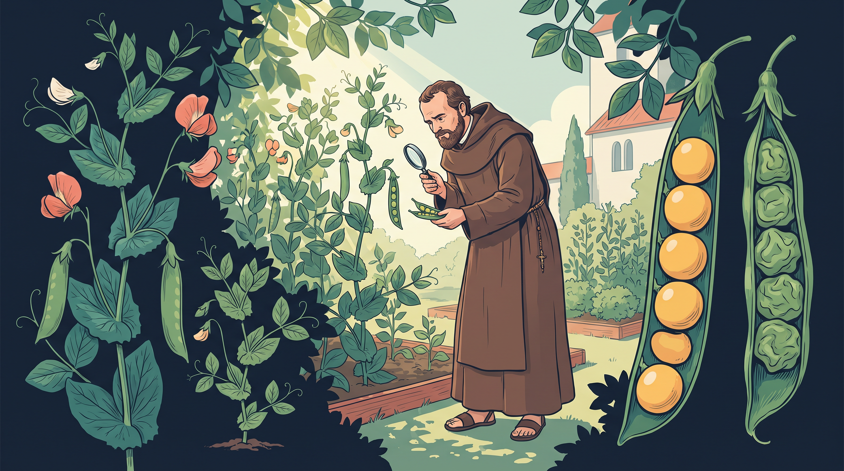
Fig. 4.0 – Gregor Mendel and the contrasting traits of garden peas.
By the end of this chapter, you will be able to answer each of these questions using the principles of inheritance and variation.
4.1 Mendel’s Laws of Inheritance
The Science of Genetics
Have you noticed that children often resemble their parents, yet are never exact copies of them? A whole branch of biology is devoted to understanding exactly this. Genetics is the branch of biology that studies how characters are passed from parents to offspring, and why offspring still differ from their parents.
Two ideas sit at the heart of this subject: inheritance and variation. Inheritance is the process by which characters are passed on from parent to progeny; it is the very basis of heredity. Variation is the degree by which progeny differ from their parents. Every family shows both at once — children carry their parents’ features (inheritance) but also show their own differences (variation).
Selective Breeding Before Science
Long before anyone understood the science behind it, humans were already putting variation to use. From as early as 8000–1000 B.C., people noticed that individual plants and animals in wild populations differed from one another, and they deliberately bred organisms that carried useful features. By repeatedly selecting and breeding such organisms — a process called artificial selection — they slowly domesticated wild species into improved forms.
A familiar example is the Sahiwal breed of cattle in Punjab, developed from wild cattle through generations of selective breeding. Our ancestors clearly recognised that characters were inherited and that variation existed, but they had very little idea about the scientific basis behind these phenomena.
Mendel and His Pea Experiments
The scientific breakthrough came in the mid-nineteenth century with Gregor Mendel. He carried out carefully planned hybridisation (cross-breeding) experiments on garden pea plants for seven years (1856–1863) and, from his results, proposed the laws of inheritance in living organisms.
Mendel’s approach was remarkable for its time. His was the first work in which statistical analysis and mathematical logic were applied to a biological problem. He worked with a large number of plants, which gave greater reliability to his data, and he confirmed his conclusions across several successive generations. Because the same results held up generation after generation, they pointed to general rules of inheritance rather than being chance, one-off observations.
Mendel deliberately chose characters that appeared in two clearly opposing forms — for example, tall or dwarf plants, and yellow or green seeds. Working with such sharply contrasting traits allowed him to build a clear framework of rules, which later scientists expanded to explain the far more complex patterns seen throughout nature.
True-Breeding Lines and Contrasting Traits
For his crosses, Mendel used several true-breeding pea lines. A true-breeding line is one that, having undergone continuous self-pollination, shows stable inheritance and expression of a trait for many generations — that is, it “breeds true” and does not throw up surprises in later generations.
Mendel selected 14 true-breeding pea varieties, arranged as pairs that were alike in every way except for one character with contrasting traits. Among the contrasting traits he studied were smooth or wrinkled seeds, yellow or green seeds, inflated (full) or constricted pods, and tall or dwarf plants. In all, he worked with seven pairs of contrasting characters, shown in Fig. 4.1 and listed in Table 4.1.
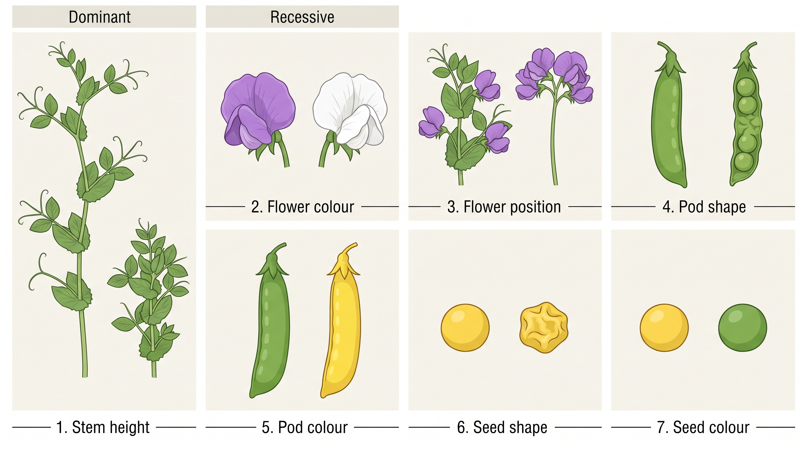
Fig. 4.1 – Seven pairs of contrasting traits in the garden pea.
Table 4.1: Contrasting Traits Studied by Mendel in Pea
| S.No. | Character | Contrasting Traits |
|---|---|---|
| 1. | Stem height | Tall / dwarf |
| 2. | Flower colour | Violet / white |
| 3. | Flower position | Axial / terminal |
| 4. | Pod shape | Inflated / constricted |
| 5. | Pod colour | Green / yellow |
| 6. | Seed shape | Round / wrinkled |
| 7. | Seed colour | Yellow / green |
This table is worth learning carefully, because the seven characters and which of their two forms is dominant are frequently tested in board and NEET papers as match-the-following or “identify the dominant trait” questions.
4.2 Inheritance of One Gene
A Cross Between Tall and Dwarf Plants
Let us follow one of Mendel’s actual experiments. He crossed a tall pea plant with a dwarf pea plant to study how a single character — height — is inherited (Fig. 4.2). To make such a cross, he first removed the anthers (the pollen-producing parts) from one flower so it could not pollinate itself — a step called emasculation — and then dusted its stigma with pollen from the other plant.
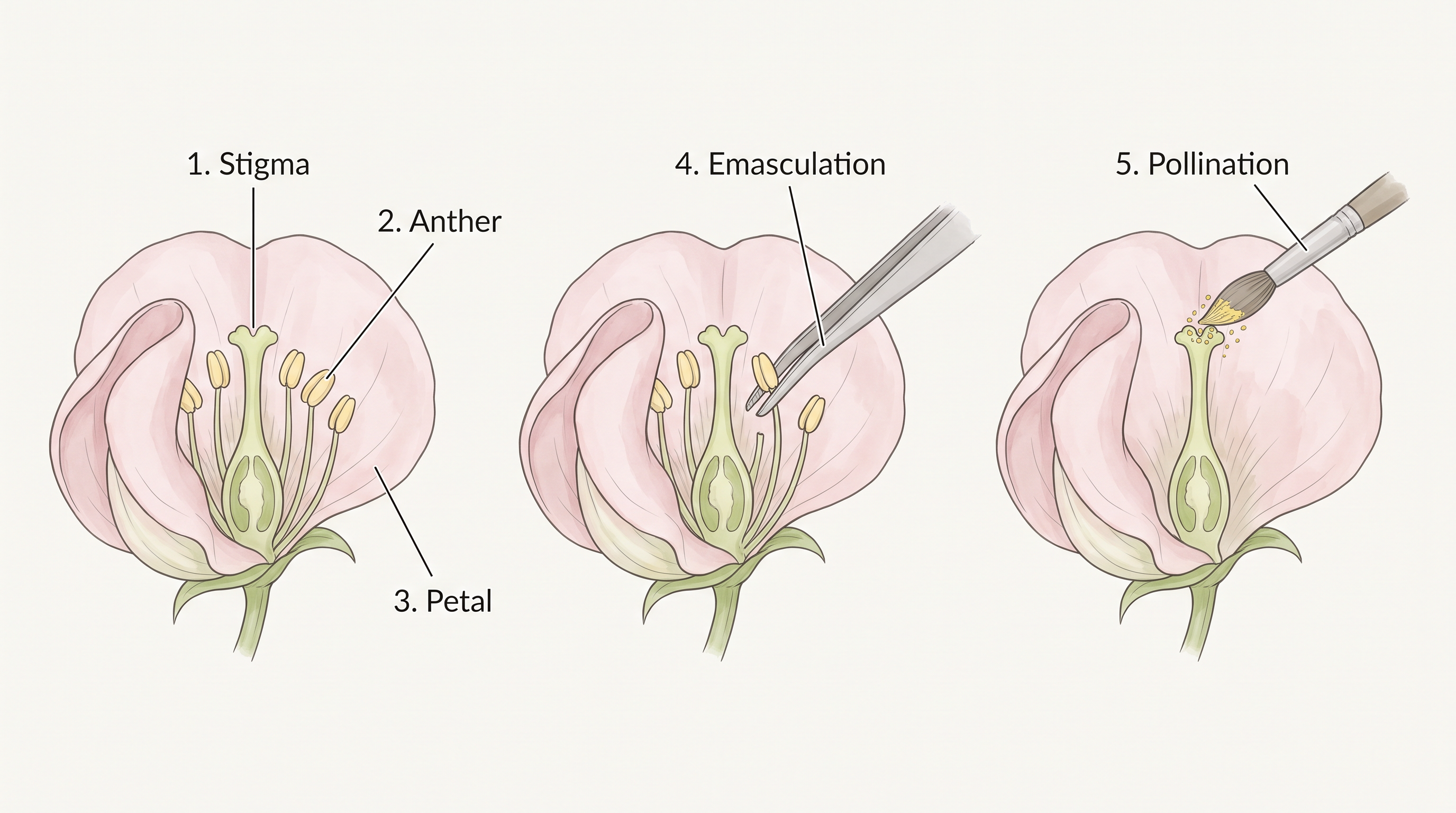
Fig. 4.2 – Steps in making a cross in a pea plant.
Mendel collected the seeds from this cross and grew them into the first hybrid generation. This generation is called the Filial₁ progeny, or simply the F₁. To his interest, every F₁ plant was tall, just like one of the parents; none were dwarf (Fig. 4.3). He saw the same pattern for the other pairs of traits: the F₁ always resembled one parent, while the trait of the other parent seemed to disappear.
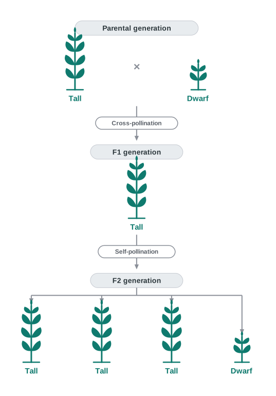
Fig. 4.3 – Diagrammatic representation of a monohybrid cross.
The Missing Trait Comes Back
Mendel then self-pollinated the tall F₁ plants. In the next generation — the Filial₂, or F₂ — something unexpected happened: some of the offspring were dwarf. The trait that had vanished in the F₁ had reappeared.
When he counted, the proportion was strikingly regular: about one-quarter (¼) of the F₂ plants were dwarf and three-quarters (¾) were tall. Just as importantly, the tall and dwarf plants were exactly like their original parental types — there was no blending. No plant was of “in-between” height; each was clearly either tall or dwarf.
He found the same result for every trait he studied: only one of the two parental traits showed up in the F₁, and at the F₂ stage both traits appeared in a ratio of 3 : 1, with no blending at either stage. This clean, repeatable 3 : 1 ratio is one of the most important observations in all of genetics.
From “Factors” to Genes
Based on these observations, Mendel proposed that something was being passed down, stably and unchanged, from parents to offspring through the gametes, generation after generation. He called these things “factors”. Today we call them genes.
Genes are the units of inheritance. They carry the information needed to express a particular trait in an organism. A gene may exist in slightly different forms that code for the contrasting versions of a trait — these alternative forms are called alleles.
Here you meet a key idea of the whole chapter — one of the questions raised at the start of it.
Symbols, Genotype and Phenotype
To keep track of alleles, we use letters. By convention, the capital letter stands for the trait expressed in the F₁ (the dominant one) and the small letter for the other trait. For height, T stands for the tall allele and t for the dwarf allele; T and t are alleles of each other.
So the possible allele pairs for height are TT, Tt or tt. In a true-breeding tall or dwarf variety, the two alleles are identical — such an individual is said to be homozygous (TT or tt). When the two alleles are different, as in Tt, the individual is heterozygous.
The actual allele composition of an organism (such as TT or tt) is its genotype, while the visible trait it shows (such as “tall” or “dwarf”) is its phenotype.
What, then, is the phenotype of a plant with genotype Tt? Mendel found that the Tt heterozygote looked exactly like the TT parent — it was tall. From this he concluded that in a pair of dissimilar factors, one factor dominates the other. The factor that expresses itself is the dominant factor; the one whose effect is hidden is the recessive factor. Here T (tall) is dominant over t (dwarf), which is recessive. He saw the same behaviour for every trait pair.
Notice why we use the capital and small form of the same letter (T and t) rather than two unrelated letters such as T and d: using the same letter makes it easy to remember that the two alleles belong to the same gene. Alleles may be similar (as in the homozygotes TT and tt) or dissimilar (as in the heterozygote Tt).
Monohybrid Cross and Segregation
Because the Tt plant is heterozygous for a single character (height), it is called a monohybrid, and a cross between TT and tt is a monohybrid cross.
The fact that the recessive dwarf trait reappears intact in the F₂, without blending, tells us something important about gamete formation. When a plant makes gametes by meiosis, the two alleles of a pair separate — or segregate — from each other, so that each gamete carries only one allele. This segregation is a random process, giving a 50 per cent chance that a gamete will carry either allele.
So a tall TT plant produces gametes all carrying T, and a dwarf tt plant produces gametes all carrying t. At fertilisation, a T-bearing gamete (say, through the pollen) unites with a t-bearing gamete (through the egg), producing a zygote with one T and one t allele — a Tt hybrid. Since this hybrid carries alleles for contrasting traits, it is heterozygous.
Flowchart
FC 4.1 – Monohybrid cross: P: TT (tall) × tt (dwarf) → gametes T and t → F1: all Tt (tall) → self-pollinate F1 → F2: 1 TT : 2 Tt : 1 tt (genotype) = 3 tall : 1 dwarf (phenotype).
The Punnett Square
The formation of gametes, their union, and the resulting F₁ and F₂ can be worked out neatly using a diagram called the Punnett square (Fig. 4.4). It was developed by the British geneticist Reginald C. Punnett. It is simply a graphical way to calculate the probability of every possible genotype among the offspring of a cross: the possible gametes of the two parents are written along the top row and the left column, and each box shows the combination that results.
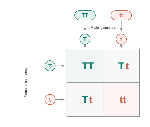
Fig. 4.4 – Punnett square for a monohybrid cross.
In the Punnett square, the F₁ Tt plant, when self-pollinated, produces T and t gametes in equal proportion (the symbols ♀ and ♂ denote the egg and pollen). A T-bearing pollen grain has a 50 per cent chance of fertilising a T-bearing egg and a 50 per cent chance of fertilising a t-bearing egg; the same is true for t-bearing pollen. As a result of this random fertilisation, the zygotes formed are of the genotypes TT, Tt or tt.
The square shows clearly that ¼ of the fertilisations give TT, ½ give Tt, and ¼ give tt. Although the F₁ genotype is Tt, its phenotype is “tall”. In the F₂, ¾ of the plants are tall — some of these are TT and some are Tt, and the two cannot be told apart by looking. Because only the T character shows in the Tt plants, T (tall) is said to dominate over t (dwarf).
This dominance is why all the F₁ are tall (though genetically Tt), and why in the F₂ ¾ are tall (½ Tt + ¼ TT) and ¼ are dwarf (tt). Thus the phenotypic ratio is 3 : 1, while the genotypic ratio is 1 : 2 : 1.
Expressing the Ratio Mathematically
The 1 : 2 : 1 ratio of TT : Tt : tt can be written as a binomial expression, because the gametes carrying T or t are produced in equal frequency of ½. Expanding it:
\[\left(\tfrac{1}{2}T + \tfrac{1}{2}t\right)^2 = \left(\tfrac{1}{2}T + \tfrac{1}{2}t\right) \times \left(\tfrac{1}{2}T + \tfrac{1}{2}t\right) = \tfrac{1}{4}\,TT + \tfrac{1}{2}\,Tt + \tfrac{1}{4}\,tt\]
Here each term gives the expected proportion of that genotype in the F₂.
The Test Cross
Mendel self-pollinated the F₂ plants and found that dwarf F₂ plants continued to give only dwarf offspring in the F₃ and F₄ generations. He concluded that the dwarfs were homozygous (tt). (What do you think he would have obtained had he instead self-pollinated a tall F₂ plant?)
This raises a practical difficulty. Although the genotypic ratios can be calculated by probability, simply looking at a dominant phenotype does not reveal the genotype. A tall plant from the F₁ or F₂ might be TT or Tt — we cannot tell by appearance alone.
To solve this, Mendel crossed a tall plant (whose genotype was unknown) with a dwarf plant. He called this a test cross. In a test cross, the organism showing the dominant phenotype is crossed with the homozygous recessive parent (instead of being self-crossed). The offspring can then be analysed to work out the unknown genotype. Fig. 4.5 shows a test cross for flower colour, where violet (V) is dominant over white (v).
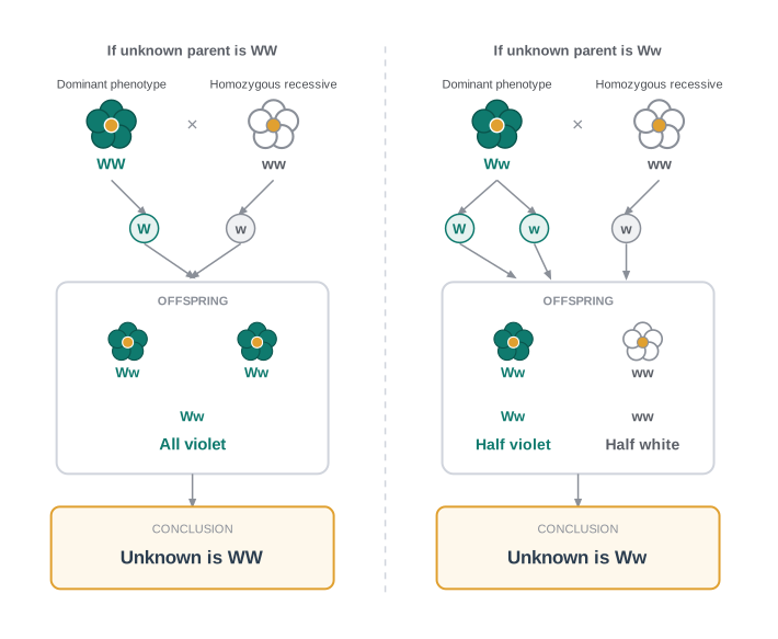
Fig. 4.5 – Diagrammatic representation of a test cross.
4.2.1 Law of Dominance
From his monohybrid crosses, Mendel drew two general rules that we today call the Principles (or Laws) of Inheritance: the First Law, the Law of Dominance, and the Second Law, the Law of Segregation.
The Law of Dominance is based on three ideas: characters are controlled by discrete units called factors; these factors occur in pairs; and in a dissimilar pair, one member dominates the other.
This law explains why only one parental character shows in the F₁ of a monohybrid cross, why both characters appear in the F₂, and why the F₂ shows the 3 : 1 phenotypic ratio.
4.2.2 Law of Segregation
The Law of Segregation is based on the fact that alleles do not blend, and that both characters are recovered unchanged in the F₂ even though one of them was hidden in the F₁. Though a parent carries two alleles, these separate during gamete formation so that each gamete receives only one of the two.
A homozygous parent (TT or tt) therefore produces only one kind of gamete, while a heterozygous parent (Tt) produces two kinds of gametes — half carrying one allele and half the other — in equal proportion.
4.2.2.1 Incomplete Dominance
When such experiments were repeated with other traits in other plants, it was found that sometimes the F₁ did not resemble either parent but was in between the two. A clear example is flower colour in the dog flower (snapdragon, Antirrhinum sp.).
In a cross between a true-breeding red-flowered plant (RR) and a true-breeding white-flowered plant (rr), the F₁ (Rr) was pink — a colour intermediate between red and white (Fig. 4.6). When this pink F₁ was self-pollinated, the F₂ appeared in the ratio 1 red (RR) : 2 pink (Rr) : 1 white (rr).
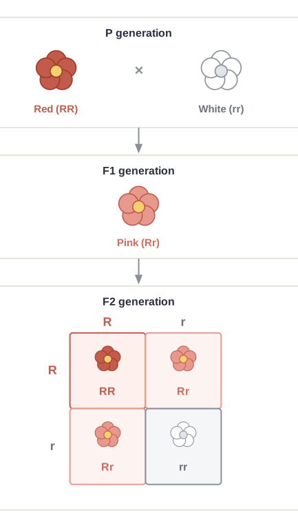
Fig. 4.6 – Incomplete dominance in snapdragon flowers.
Notice that the genotype ratio (1 : 2 : 1) is exactly what we expect in any Mendelian monohybrid cross, but the phenotype ratio has changed from 3 : 1 to 1 : 2 : 1. This happens because R is not completely dominant over r; the heterozygote Rr shows its own intermediate (pink) phenotype, which is distinct from both RR (red) and rr (white).
To understand why an allele may be dominant or recessive, we must ask what a gene actually does. Every gene carries the information to express a trait. In a diploid organism there are two copies of each gene — a pair of alleles — and these need not be identical; one may have undergone a change (a modification) that alters the information it carries.
Consider a gene that carries the information for making an enzyme needed to convert a substrate S. There are two allelic forms. Suppose the normal allele makes the normal, working enzyme. The modified allele could then be responsible for producing, in theory, one of three things: (i) the normal (or a less efficient) enzyme, or (ii) a non-functional enzyme, or (iii) no enzyme at all.
In the first case, the modified allele behaves just like the normal allele — it still allows substrate S to be transformed — so such equivalent allele pairs are very common and no difference is seen. But if the modified allele makes a non-functional enzyme or no enzyme, then the phenotype depends entirely on the normal, working allele. The normal (functioning) allele, which produces the original phenotype, then behaves as the dominant allele, while the modified allele behaves as the recessive one. In other words, in the example above the recessive trait appears precisely because the modified allele makes a faulty enzyme or no enzyme.
4.2.2.2 Co-dominance
So far we have seen crosses where the F₁ either resembled one parent (complete dominance) or was intermediate between the two (incomplete dominance). In co-dominance, the F₁ resembles both parents at the same time — both alleles express themselves fully and independently.
A good example is the different types of red blood cells that determine ABO blood grouping in humans. ABO blood groups are controlled by the gene I. The plasma membrane of red blood cells carries sugar polymers that stick out from its surface, and the kind of sugar made is controlled by this gene.
The gene I has three alleles: \(I^A\), \(I^B\) and i. The alleles \(I^A\) and \(I^B\) each produce a slightly different form of the surface sugar, while the allele i produces no sugar at all. Because humans are diploid, each person carries any two of these three alleles.
Both \(I^A\) and \(I^B\) are completely dominant over i. So when \(I^A\) and i are present together, only \(I^A\) expresses (because i makes no sugar), giving blood group A; and when \(I^B\) and i are together, \(I^B\) expresses, giving group B. But when \(I^A\) and \(I^B\) are present together, both express their own sugars — this is co-dominance — so the red blood cells carry both A and B sugars, giving blood group AB.
Since there are three different alleles, there are six possible combinations of two alleles, giving six different genotypes but only a smaller number of blood-group phenotypes (Table 4.2). How many phenotypes are possible?
Table 4.2: Genetic Basis of Blood Groups in the Human Population
| Allele from Parent 1 | Allele from Parent 2 | Genotype of offspring | Blood type of offspring |
|---|---|---|---|
| \(I^A\) | \(I^A\) | \(I^A I^A\) | A |
| \(I^A\) | \(I^B\) | \(I^A I^B\) | AB |
| \(I^A\) | i | \(I^A i\) | A |
| \(I^B\) | \(I^A\) | \(I^A I^B\) | AB |
| \(I^B\) | \(I^B\) | \(I^B I^B\) | B |
| \(I^B\) | i | \(I^B i\) | B |
| i | i | i i | O |
Here is the answer to another question raised at the start of the chapter.
The ABO example also illustrates multiple alleles: here there are more than two — in fact three — alleles (\(I^A\), \(I^B\), i) governing the same character. Since an individual can carry only two alleles at a time, the existence of multiple alleles for a gene can be recognised only when a whole population is studied.
Finally, a single gene product may sometimes influence more than one feature. For example, starch synthesis in pea seeds is controlled by one gene with two alleles (B and b). Starch is synthesised effectively by BB homozygotes, which produce large starch grains, whereas bb homozygotes are less efficient and produce smaller grains. After the seeds mature, BB seeds are round and bb seeds are wrinkled, and the heterozygote Bb produces round seeds — so, judged by seed shape, B appears dominant. However, the starch grains in Bb seeds are of intermediate size, so if starch-grain size is taken as the phenotype, the alleles show incomplete dominance.
This leads to an important idea: dominance is not a fixed, automatic property of a gene. Whether an allele appears dominant depends both on the gene product and on which particular phenotype we choose to examine when a single gene affects more than one feature.
4.3 Inheritance of Two Genes
A Cross Following Two Characters at Once
Mendel did not stop at single characters. He also crossed pea plants that differed in two characters at the same time. In one such cross, he took a plant with round, yellow seeds and crossed it with a plant having wrinkled, green seeds (Fig. 4.7). The seeds produced by this cross were all round and yellow. (Can you already tell, from this result, which trait in each pair was dominant?)
The answer is that yellow was dominant over green, and round was dominant over wrinkled — exactly the same as when Mendel made separate monohybrid crosses for seed colour and for seed shape.
Let us use symbols: Y for dominant yellow and y for recessive green; R for round and r for wrinkled. The parents are then RRYY (round yellow) and rryy (wrinkled green). The gametes RY and ry unite at fertilisation to give the F₁ hybrid RrYy, which is round and yellow.
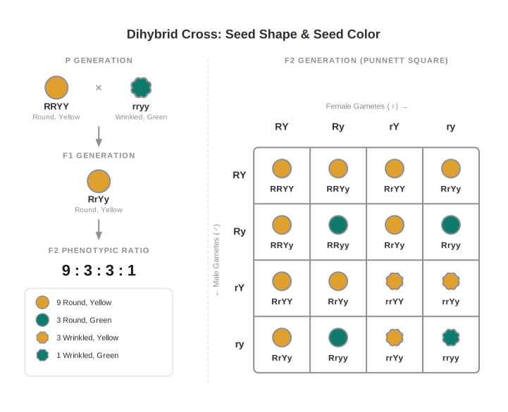
Fig. 4.7 – Punnett square for a dihybrid cross.
When Mendel self-pollinated these F₁ plants, he found that ¾ of the F₂ plants had yellow seeds and ¼ had green — a 3 : 1 ratio for colour. Independently, round and wrinkled seed shape also appeared in a 3 : 1 ratio, just as in a monohybrid cross. A plant that is heterozygous for two characters, like RrYy, is called a dihybrid, and a cross between such plants is a dihybrid cross.
Flowchart
FC 4.2 – Dihybrid cross: P: RRYY (round yellow) × rryy (wrinkled green) → gametes RY and ry → F1: all RrYy (round yellow) → self-pollinate F1 → gametes RY, Ry, rY, ry (each ¼) → F2: 9 round yellow : 3 round green : 3 wrinkled yellow : 1 wrinkled green.
4.3.1 Law of Independent Assortment
In the dihybrid cross, the four phenotypes — round yellow, round green, wrinkled yellow, and wrinkled green — appeared in the ratio 9 : 3 : 3 : 1. Mendel found this same ratio for several pairs of characters.
This 9 : 3 : 3 : 1 ratio can be understood as a combination of two separate 3 : 1 ratios:
\[(3\ \text{round} : 1\ \text{wrinkled}) \times (3\ \text{yellow} : 1\ \text{green})\] \[= 9\ \text{round, yellow} : 3\ \text{wrinkled, yellow} : 3\ \text{round, green} : 1\ \text{wrinkled, green}\]
From such observations on dihybrid crosses (crosses between plants differing in two traits), Mendel proposed a second general rule — Mendel’s Law of Independent Assortment.
To see how this works, use the Punnett square for the F₁ RrYy plant. Consider first the R/r pair: 50 per cent of the gametes carry R and 50 per cent carry r. Now, besides carrying R or r, each gamete must also carry either Y or y. The key point is that the 50 : 50 split of R and r is independent of the 50 : 50 split of Y and y.
So, of the r-bearing gametes, half carry Y and half carry y; and of the R-bearing gametes, half carry Y and half carry y. This gives four types of gametes — RY, Ry, rY and ry — each with a frequency of 25 per cent (¼) of all gametes produced. The same four types form in both the pollen and the eggs.
When these four types of eggs and pollen are placed on the two sides of a Punnett square, the 16 boxes give the F₂ zygotes (Fig. 4.7).
4.3.2 Chromosomal Theory of Inheritance
Mendel published his work on inheritance in 1865, but for several reasons it went unrecognised until 1900.
Why Mendel’s Work Was Overlooked
There were four main reasons. First, communication was slow in those days, so his work was not widely publicised. Second, his idea of genes (factors) as stable, discrete units that did not “blend” was not accepted by contemporaries, who believed in the smooth, continuous variation seen in nature. Third, his use of mathematics to explain a biological phenomenon was completely new and unwelcome to many biologists of the time. Finally, although his work suggested that factors were discrete units, he could offer no physical proof of their existence or say what they were made of.
In 1900, three scientists — de Vries, Correns and von Tschermak — independently rediscovered Mendel’s results. Around the same time, improvements in microscopy allowed scientists to observe cell division carefully, and they discovered thread-like structures in the nucleus that appeared to double and then divide just before each cell division. These were named chromosomes (meaning “coloured bodies”, because they took up stain and became visible).
Linking Chromosomes to Mendel’s Factors
By 1902, the movement of chromosomes during meiosis had been worked out. Walter Sutton and Theodore Boveri noticed that the behaviour of chromosomes ran exactly parallel to the behaviour of Mendel’s genes, and they used chromosome movement (Fig. 4.8) to explain Mendel’s laws (Table 4.3).
Recall from your study of cell division that chromosomes behave in a particular way during mitosis (equational division) and meiosis (reduction division). The important points are that chromosomes, like genes, occur in pairs, and that the two alleles of a gene pair sit at the same (homologous) positions on the two homologous chromosomes.
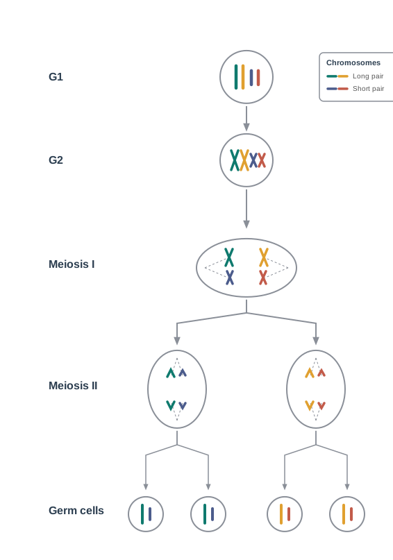
Fig. 4.8 – Chromosome segregation during meiosis.
Table 4.3: A Comparison Between the Behaviour of Chromosomes and Genes
| A | B |
|---|---|
| Occur in pairs | Occur in pairs |
| Segregate at gamete formation such that only one of each pair is transmitted to a gamete | Segregate at gamete formation and only one of each pair is transmitted to a gamete |
| Independent pairs segregate independently of each other | One pair segregates independently of another pair |
How Chromosomes Assort Independently
During anaphase of meiosis I, the two chromosome pairs can line up at the metaphase plate independently of each other (Fig. 4.9). If you compare four chromosomes of different colours, in one possibility the orange chromosome segregates together with the green one, while in another possibility the orange chromosome segregates with the red one. This physical independence of chromosome alignment is the cellular basis of Mendel’s Law of Independent Assortment.
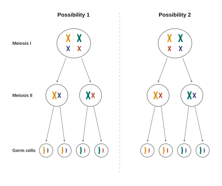
Fig. 4.9 – Independent assortment of chromosomes.
Morgan and the Fruit Fly
Following Sutton and Boveri’s synthesis of ideas, the chromosomal theory was experimentally verified by Thomas Hunt Morgan and his colleagues, whose work revealed the basis of the variation produced by sexual reproduction.
Morgan worked with the tiny fruit fly, Drosophila melanogaster (Fig. 4.10), which proved ideal for genetic studies for several reasons: the flies could be grown on a simple synthetic medium in the laboratory; they complete their life cycle in about two weeks; a single mating produces a large number of offspring; the two sexes are easy to tell apart; and the flies show many hereditary variations that can be seen even under a low-power microscope.
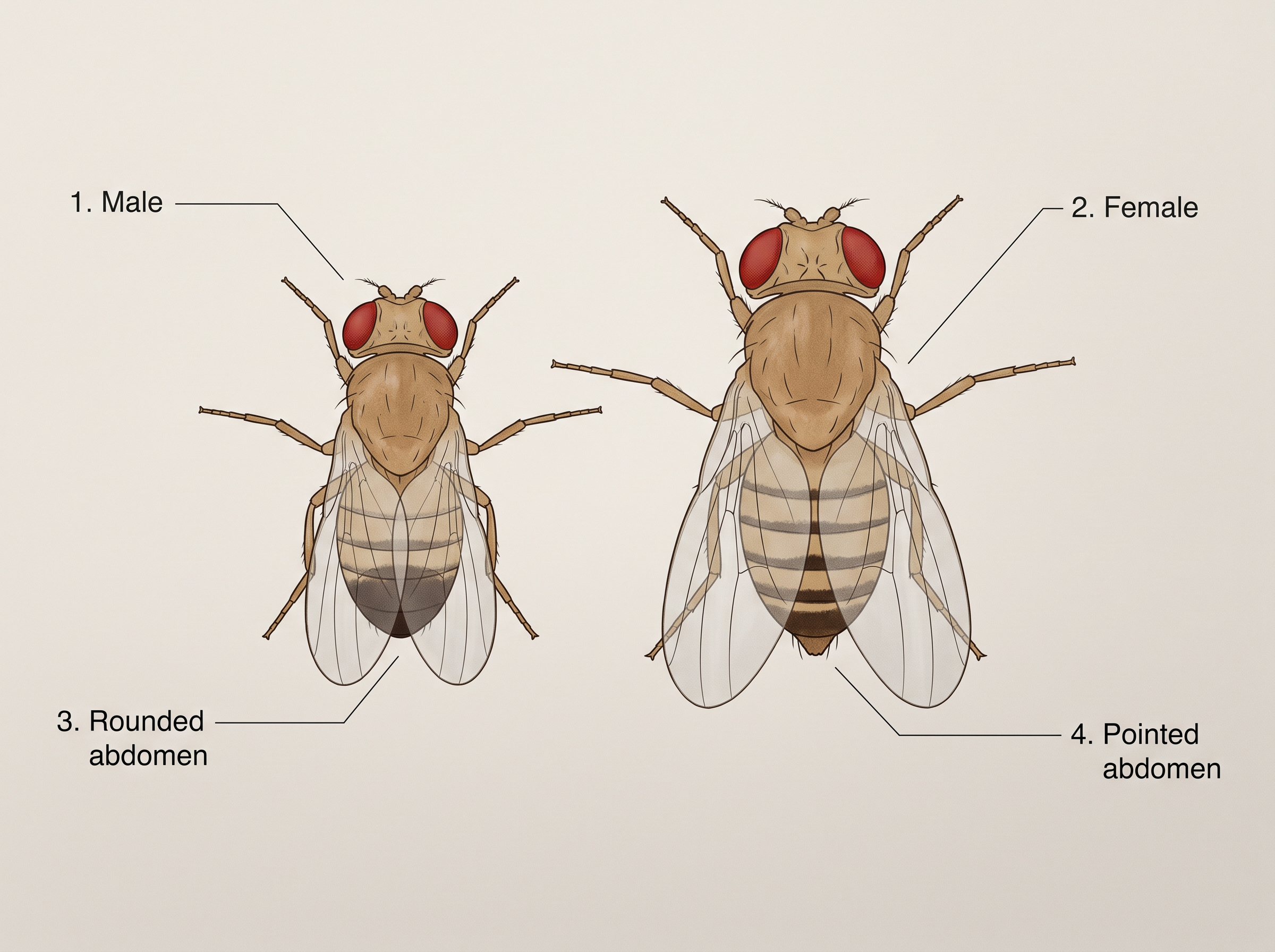
Fig. 4.10 – Male and female Drosophila melanogaster.
4.3.3 Linkage and Recombination
Morgan carried out several dihybrid crosses in Drosophila to study genes that were sex-linked (located on the sex chromosomes). His crosses were similar to Mendel’s dihybrid crosses in peas. For example, he crossed yellow-bodied, white-eyed females with brown-bodied, red-eyed males, and intercrossed their F₁. He found that the two genes did not assort independently, and the F₂ ratio deviated sharply from the 9 : 3 : 3 : 1 expected when two genes are independent.
Morgan and his group knew that these genes were located on the same (X) chromosome — the sex chromosomes are discussed in Section 4.6. They saw that when two genes in a dihybrid cross lie on the same chromosome, the parental combinations of genes appear far more often than the non-parental ones.
Morgan explained this by the physical association of the two genes on the chromosome, which he called linkage. He used the term recombination for the appearance of the non-parental gene combinations (Fig. 4.11).

Fig. 4.11 – Linkage and recombination in Drosophila.
Morgan and his group also found that even genes grouped on the same chromosome were not all linked to the same degree. Some genes were very tightly linked, showing very low recombination (Fig. 4.11, Cross A), while others were loosely linked, showing higher recombination (Fig. 4.11, Cross B). For example, the genes white and yellow were very tightly linked and showed only 1.3 per cent recombination, whereas white and miniature wing showed 37.2 per cent recombination.
Morgan’s student Alfred Sturtevant used the frequency of recombination between gene pairs on the same chromosome as a measure of the distance between them, and in this way “mapped” their positions on the chromosome. Such genetic maps are still used today as a starting point for sequencing whole genomes, as was done in the Human Genome Sequencing Project (described later).
4.4 Polygenic Inheritance
When Traits Come in a Range, Not Just Two Types
Most of the traits Mendel studied had two sharply distinct forms — a flower was either violet or white, a plant either tall or dwarf. But if you look around, you will notice many traits that are not so neatly divided. Human height, for instance, is not simply “tall” or “short”; people show a whole continuous range of heights.
Such traits are usually controlled by three or more genes, and are therefore called polygenic traits. Their pattern of inheritance is called polygenic inheritance.
Besides involving several genes, polygenic inheritance is also influenced by the environment. Height, for example, depends not only on genes but also on factors such as nutrition and health during growth. Human skin colour is another classic example of a polygenic trait.
How Additive Effects Work
In a polygenic trait, the phenotype reflects the contribution of each allele — that is, the effect of each allele is additive. Each “dominant-type” allele adds a small amount to the trait, so the total number of such alleles decides where an individual falls within the range.
To see this, suppose three genes A, B and C control skin colour in humans, with the dominant forms A, B and C responsible for dark skin and the recessive forms a, b and c for light skin. Then: - The genotype with all dominant alleles (AABBCC) gives the darkest skin. - The genotype with all recessive alleles (aabbcc) gives the lightest skin. - A genotype with three dominant and three recessive alleles gives an intermediate skin colour.
In this way, the number of each type of allele present in the genotype determines how dark or light the skin of an individual is.
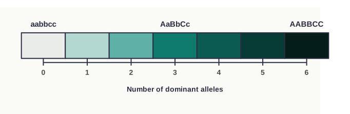
Fig. 4.12a – Additive basis of a polygenic trait.
4.5 Pleiotropy
One Gene, Many Effects
In every case so far, we have looked at how a gene affects a single trait. But sometimes the opposite of polygenic inheritance happens: a single gene can influence several different traits at once. Such a gene is called a pleiotropic gene, and this phenomenon is called pleiotropy.
How can one gene affect many traits? In most cases the gene acts on a metabolic pathway — a series of linked chemical reactions in the body — and a single change in that one pathway then shows up as several different phenotypes.
Phenylketonuria: A Pleiotropic Example
A clear example in humans is the disease phenylketonuria. It is caused by a mutation in the single gene that codes for the enzyme phenylalanine hydroxylase. Even though only one gene is faulty, the disease shows itself through more than one effect — it is marked both by mental retardation and by a reduction in hair and skin pigmentation.
The reason a single faulty gene produces these different effects is that the missing enzyme normally works within a metabolic pathway; when it fails, that one disturbance ripples outward and appears as several separate phenotypes.
Flowchart
FC 4.3 – Pleiotropy in phenylketonuria: mutation in the single gene for phenylalanine hydroxylase → enzyme non-functional → one disturbed metabolic pathway → branches into two phenotypes: (a) effects on the brain → mental retardation, and (b) reduced pigment formation → reduced hair and skin pigmentation.
4.6 Sex Determination
An Early Clue from Insects
For a long time, how the sex of an organism is decided was a puzzle for geneticists. The first clue came from experiments on insects. The German biologist Henking (1891) traced a particular nuclear structure right through the process of sperm formation (spermatogenesis) in a few insects, and noticed that exactly 50 per cent of the sperm received this structure while the other 50 per cent did not. He called it the X body, but could not explain what it meant.
Further study revealed that in many insects, sex determination is of the XO type: all eggs carry an extra X-chromosome besides the other chromosomes (the autosomes), but only some of the sperm carry an X-chromosome while others do not. An egg fertilised by an X-bearing sperm becomes a female, and an egg fertilised by a sperm without an X becomes a male.
Because the X-chromosome was involved in deciding sex, it was named a sex chromosome, and all the remaining chromosomes were called autosomes.
The grasshopper is a good example of the XO type: males have only a single X-chromosome besides the autosomes, whereas females have a pair of X-chromosomes.
XY Type and the Idea of Heterogamety
These findings led scientists to examine many species. In a number of other insects and in mammals, including humans, sex determination is of the XY type, where both males and females have the same number of chromosomes. Here the male has one X-chromosome, but its partner is distinctly smaller and is called the Y-chromosome; females have a pair of X-chromosomes. Both sexes carry the same set of autosomes. So males have autosomes plus XY, while females have autosomes plus XX. This is the case in human beings and in Drosophila (Fig. 4.13 a, b).
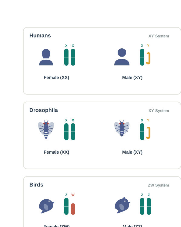
Fig. 4.13 – Sex determination in humans, fruit flies and birds.
In both the XO and XY types, the male produces two different kinds of gametes — either with or without an X-chromosome (XO type), or some carrying X and some carrying Y (XY type). This is called male heterogamety.
In some organisms, such as birds, a different mechanism operates (Fig. 4.13 c). Here the total number of chromosomes is the same in both sexes, but it is the female that produces two different kinds of gametes with respect to the sex chromosome — this is called female heterogamety. To distinguish this system from the earlier one, the two sex chromosomes of the female bird are named Z and W. In these organisms, the female has one Z and one W chromosome, whereas the male has a pair of Z-chromosomes besides the autosomes.
4.6.1 Sex Determination in Humans
In humans, sex determination is of the XY type. Of the 23 pairs of chromosomes present, 22 pairs are exactly the same in both males and females — these are the autosomes. The remaining pair is the sex chromosomes: females have a pair of X-chromosomes (XX), while males have one X and one Y chromosome (XY).
During spermatogenesis in males, two types of sperm are produced: 50 per cent carry the X-chromosome and 50 per cent carry the Y-chromosome, besides the autosomes. Females, however, produce only one type of ovum, all carrying an X-chromosome.
There is an equal chance that an ovum is fertilised by a sperm carrying either X or Y. If the ovum is fertilised by an X-bearing sperm, the zygote develops into a female (XX); if it is fertilised by a Y-bearing sperm, it develops into a male (XY). It is therefore clear that it is the genetic makeup of the sperm that determines the sex of the child, and that in each pregnancy there is always a 50 per cent probability of either a male or a female child.
Flowchart
FC 4.4 – Human sex determination: sperm carries either X or Y (50% each); ovum always carries X → X-sperm + X-ovum → XX (girl); Y-sperm + X-ovum → XY (boy); each pregnancy → 50% girl : 50% boy.
Here is the answer to a question raised at the start of the chapter.
4.6.2 Sex Determination in Honey Bee
The honey bee uses a completely different mechanism, based not on particular sex chromosomes but on the number of chromosome sets an individual receives.
An offspring formed from the union of a sperm and an egg (a fertilised egg) develops into a female — a queen or a worker. An unfertilised egg develops into a male (a drone) by a process called parthenogenesis, the development of an offspring from an unfertilised egg.
This means the males have half the number of chromosomes that a female has. The females are diploid, with 32 chromosomes, while the males are haploid, with 16 chromosomes. Because sex here depends on being haploid or diploid, the system is called the haplodiploid sex-determination system.
Flowchart
FC 4.5 – Honey bee (haplodiploidy): fertilised egg (sperm + egg) → diploid (2n = 32 chromosomes) → female (queen or worker); unfertilised egg → develops by parthenogenesis → haploid (n = 16 chromosomes) → male (drone).
This system produces some unusual features. Because males develop from unfertilised eggs, they produce their sperm by mitosis (not meiosis), they have no father and therefore cannot have sons — yet they can have a grandfather and can have grandsons.
4.7 Mutation
What Is a Mutation?
Mutation is a change (alteration) in the DNA sequence, which then leads to changes in the genotype and phenotype of an organism. Along with recombination — which you met earlier in this chapter — mutation is one of the main ways in which variation arises in DNA.
Chromosome-Level Changes
As you will study in Chapter 5, in each chromatid a single DNA helix runs continuously from one end to the other in a highly coiled (supercoiled) form. So if a segment of DNA is lost (a deletion) or gained (an insertion or duplication), the chromosome itself becomes altered.
Because genes lie on chromosomes, such alterations of chromosomes lead to abnormalities called chromosomal aberrations. These aberrations are commonly seen in cancer cells.
Gene-Level Changes: Point and Frame-shift Mutations
Mutation can also arise from a change in a single base pair of DNA. This is called a point mutation. A classical example of a point mutation is sickle-cell anaemia (its details are discussed in Section 4.8).
When base pairs are inserted or deleted, the whole “reading frame” of the DNA is shifted, producing what are called frame-shift mutations (you will study these further in Chapter 5).
Flowchart
FC 4.6 – Types of mutation: mutation → (a) chromosome level: deletion / insertion / duplication of a DNA segment → chromosomal aberration; (b) gene level: change in a single base pair → point mutation (e.g., sickle-cell anaemia); or insertion / deletion of base pairs → frame-shift mutation.
What Causes Mutations?
The detailed mechanism of mutation is beyond our present scope. However, we do know that many chemical and physical factors can bring about, or induce, mutations. Such mutation-causing agents are called mutagens. For example, UV (ultraviolet) radiation can cause mutations in organisms, and is therefore a mutagen.
4.8 Genetic Disorders
4.8.1 Pedigree Analysis
The idea that disorders can be inherited has existed in human society for a very long time, based on the observation that certain features run in families. After Mendel’s work was rediscovered, people began to study inheritance patterns in humans in the same scientific way.
There is, however, a practical problem. The controlled crosses that can be made with pea plants or other organisms are obviously not possible with human beings. Instead, biologists study the family history of a particular trait across several generations. This method is called pedigree analysis: the inheritance of a trait is represented in a family tree spread over generations.
Pedigree analysis is a powerful tool used to trace the inheritance of a specific trait, abnormality or disease in humans. It uses a set of standard symbols to represent individuals and relationships (Fig. 4.14a).
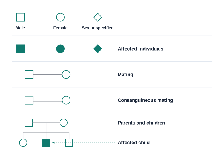
Fig. 4.14a – Standard symbols in pedigree analysis.
Every feature of an organism is controlled by one or another gene located on the DNA in its chromosomes. DNA is the carrier of genetic information, and it is normally transmitted from one generation to the next without change. Occasionally, though, a change does occur in the genetic material — such a change is called a mutation. A number of human disorders are found to be associated with the inheritance of such changed or altered genes or chromosomes.
4.8.2 Mendelian Disorders
Broadly, genetic disorders fall into two categories — Mendelian disorders and chromosomal disorders.
Mendelian disorders are caused mainly by an alteration or mutation in a single gene. They are passed to offspring along the same lines as the principles of inheritance you studied earlier, so their inheritance pattern can be traced in a family by pedigree analysis.
Some of the most common and prevalent Mendelian disorders are haemophilia, cystic fibrosis, sickle-cell anaemia, colour blindness, phenylketonuria and thalassemia. Such disorders may be dominant or recessive, and pedigree analysis can reveal which. A disorder may also be linked to the sex chromosome, as in haemophilia, which is an X-linked recessive trait passed from a carrier female to some of her sons. Representative pedigrees for a dominant and a recessive trait are shown in Fig. 4.15.
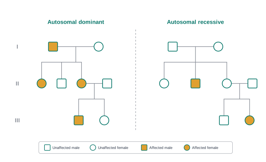
Fig. 4.15 – Pedigree analysis of dominant and recessive traits.
Flowchart
FC 4.8 – Classification of genetic disorders: genetic disorders → (a) Mendelian disorders (single-gene mutation; may be dominant or recessive; e.g., haemophilia, cystic fibrosis, sickle-cell anaemia, colour blindness, phenylketonuria, thalassemia); (b) chromosomal disorders (absence / excess / abnormal arrangement of chromosomes → aneuploidy, e.g., Down’s, Turner’s, Klinefelter’s; or polyploidy).
Before looking at individual disorders, one useful term is carrier — a person who has a recessive disease allele but does not show the disease.
Colour Blindness
Colour blindness is a sex-linked recessive disorder caused by a defect in either the red or the green cone cells of the eye, resulting in a failure to tell red and green apart. The defect is due to a mutation in certain genes present on the X chromosome.
It occurs in about 8 per cent of males but only about 0.4 per cent of females. The reason lies in the number of X chromosomes: males have only one X chromosome, whereas females have two. A son of a woman who carries the gene has a 50 per cent chance of being colour blind. The mother herself is usually not colour blind, because the recessive gene’s effect is masked by her matching dominant normal gene. A daughter will not normally be colour blind unless her mother is a carrier and her father is colour blind.
Here is the answer to one of the questions raised at the start of the chapter.
Haemophilia
Haemophilia is a widely studied sex-linked recessive disease, transmitted from an unaffected carrier female to some of her sons. In this disease, a single protein that is part of the cascade of proteins involved in the clotting of blood is affected. As a result, in an affected person even a simple cut leads to non-stop bleeding.
A heterozygous female (carrier) may transmit the disease to her sons. The chance of a female actually being haemophilic is extremely rare, because for that to happen her mother must be at least a carrier and her father must be haemophilic (which is usually not viable in later life).
Sickle-cell Anaemia
Sickle-cell anaemia is an autosome-linked recessive trait. It is transmitted to offspring only when both parents are carriers (heterozygous) for the gene. The disease is controlled by a single pair of alleles, \(Hb^A\) and \(Hb^S\).
Of the three possible genotypes, only the homozygous individuals \(Hb^S Hb^S\) actually show the diseased phenotype. Heterozygous individuals (\(Hb^A Hb^S\)) appear apparently unaffected, but they are carriers, with a 50 per cent chance of passing the mutant gene to their offspring — this heterozygous condition is called the sickle-cell trait (Fig. 4.16).
The defect is caused by the substitution of the amino acid glutamic acid (Glu) by valine (Val) at the sixth position of the beta-globin chain of the haemoglobin molecule (haemoglobin is the oxygen-carrying protein of red blood cells). This substitution results from a single base change at the sixth codon of the beta-globin gene, from GAG to GUG. The mutant haemoglobin molecule then polymerises under low oxygen tension, changing the shape of the red blood cell from a biconcave disc to an elongated, sickle-like structure (Fig. 4.16).
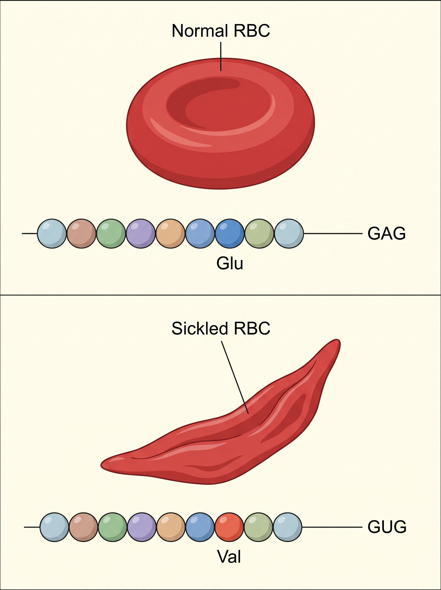
Fig. 4.16 – Red blood cells and β-globin chains in sickle-cell anaemia.
Flowchart
FC 4.7 – Molecular basis of sickle-cell anaemia: single base substitution in the β-globin gene (GAG → GUG) → glutamic acid (Glu) replaced by valine (Val) at the 6th position of the β-globin chain → abnormal haemoglobin (\(Hb^S\)) → polymerises under low oxygen tension → RBC changes from biconcave disc to elongated sickle shape → sickle-cell anaemia.
This directly answers the last of the questions raised at the start of the chapter.
Phenylketonuria
We met phenylketonuria earlier as an example of pleiotropy; here we look at how it is inherited. This inborn error of metabolism is inherited as an autosomal recessive trait. The affected individual lacks the enzyme that converts the amino acid phenylalanine into tyrosine.
As a result, phenylalanine accumulates and is converted into phenylpyruvic acid and other derivatives. The accumulation of these substances in the brain leads to mental retardation. They are also excreted in the urine, because the kidney absorbs them poorly.
Thalassemia
Thalassemia is also an autosome-linked recessive blood disease, transmitted to offspring when both parents are unaffected carriers of the gene. The defect may be due to a mutation or deletion that reduces the rate of synthesis of one of the globin chains (the α and β chains) that make up haemoglobin. This leads to the formation of abnormal haemoglobin molecules and results in the anaemia that is characteristic of the disease.
Thalassemia is classified according to which globin chain is affected. In α-thalassemia, the production of the α-globin chain is affected. It is controlled by two closely linked genes, HBA1 and HBA2, on chromosome 16 of each parent, and it arises due to mutation or deletion of one or more of these four genes — the more genes affected, the fewer α-globin molecules produced. In β-thalassemia, the production of the β-globin chain is affected. It is controlled by a single gene, HBB, on chromosome 11 of each parent, and occurs due to mutation of one or both of these genes.
Note the key distinction stated in the table: thalassemia is a quantitative problem (too few globin molecules are made), whereas sickle-cell anaemia is a qualitative problem (an incorrectly functioning globin is made).
4.8.3 Chromosomal Disorders
Chromosomal disorders are caused by the absence, excess, or abnormal arrangement of one or more whole chromosomes.
When chromatids fail to segregate properly during the cell-division cycle, an individual may gain or lose a chromosome — this is called aneuploidy. For example, Down’s syndrome results from the gain of an extra copy of chromosome 21, while Turner’s syndrome results from the loss of an X chromosome in human females. On the other hand, if cytokinesis fails after the telophase stage of cell division, the whole set of chromosomes is increased — this is called polyploidy, a condition often seen in plants.
The normal human cell has 46 chromosomes (23 pairs) — 22 pairs of autosomes and one pair of sex chromosomes. Rarely, an individual may have an additional copy of a chromosome, or may lack one of a pair; these situations are called trisomy and monosomy respectively, and both can lead to serious consequences. Down’s, Turner’s and Klinefelter’s syndromes are common examples of chromosomal disorders.
Down’s Syndrome
Down’s syndrome is caused by the presence of an additional copy of chromosome number 21 (trisomy of 21). The affected individual is short-statured with a small round head, a furrowed tongue and a partially open mouth (Fig. 4.17). The palm is broad, with a characteristic palm crease, and physical, psychomotor and mental development is retarded.
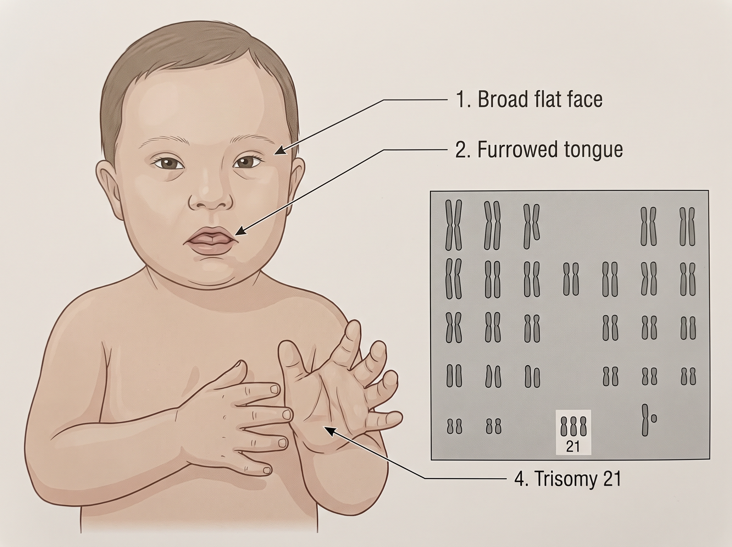
Fig. 4.17 – Down’s syndrome and the trisomy 21 karyotype.
Klinefelter’s Syndrome
Klinefelter’s syndrome is caused by the presence of an additional copy of the X chromosome, resulting in a karyotype of 47, XXY. Such an individual has an overall masculine build, but feminine features also develop — including the development of breasts, a condition called gynaecomastia. Such individuals are sterile (Fig. 4.18 a).
Turner’s Syndrome
Turner’s syndrome is caused by the absence of one of the X chromosomes, giving a karyotype of 45, X0. Such females are sterile because the ovaries are rudimentary, and they also lack other secondary sexual characters (Fig. 4.18 b).
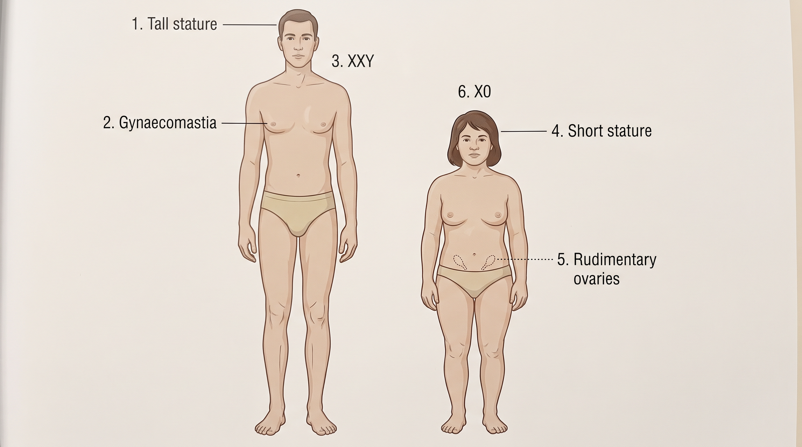
Fig. 4.18 – Klinefelter’s and Turner’s syndromes.
4.9 Summary
Genetics is the branch of biology that deals with the principles of inheritance and their practical application. The resemblance of offspring to their parents has interested biologists for a long time.
Mendel was the first to study inheritance systematically. Working with pea plants that showed contrasting characters, he proposed the rules we now call Mendel’s Laws of Inheritance.
Mendel proposed that the “factors” (later named genes) controlling characters occur in pairs, known as alleles. The characters appear in a definite pattern across generations (F₁, F₂, and so on).
Some characters are dominant over others. A dominant character is expressed even in the heterozygous condition (Law of Dominance), while a recessive character is expressed only in the homozygous condition. Characters do not blend in the heterozygote; a recessive character that is hidden in the heterozygous condition reappears when the individual becomes homozygous. Hence, alleles segregate during gamete formation (Law of Segregation).
Not all characters show complete dominance. Some show incomplete dominance (the heterozygote is intermediate, as pink in snapdragon), and some show co-dominance (both alleles express fully, as in the AB blood group). The ABO gene also illustrates multiple alleles.
When two characters are studied together (a dihybrid cross), the two pairs of factors assort independently in all combinations (Law of Independent Assortment), giving a 9 : 3 : 3 : 1 ratio. The possible gamete combinations are worked out using the Punnett square. The factors (genes) on the chromosomes make up the genotype, and their visible expression is the phenotype.
Once genes were known to lie on chromosomes, a clear link was drawn between Mendel’s laws and the segregation and assortment of chromosomes during meiosis — the Chromosomal Theory of Inheritance.
Genes located on the same chromosome do not follow independent assortment. These are linked genes: closely placed genes are inherited together, while distantly placed genes are separated by recombination. The frequency of recombination is used to prepare linkage (genetic) maps.
Many genes are sex-linked. The chromosomes that differ between the sexes are the sex chromosomes; the rest are autosomes. In humans, a female has 22 pairs of autosomes and XX, and a male has 22 pairs of autosomes and XY. In chicken (birds), the male is ZZ and the female is ZW.
Mutation is a change in the genetic material. A point mutation is a change of a single base pair in DNA — for example, sickle-cell anaemia is caused by a single base change in the gene coding for the β-chain of haemoglobin. Inheritable mutations can be studied by drawing a pedigree of a family.
Some mutations involve whole sets of chromosomes (polyploidy) or a change in part of the chromosome number (aneuploidy). This helped in understanding the basis of genetic disorders. Down’s syndrome is due to trisomy of chromosome 21 (total 47); in Turner’s syndrome one X is missing (X0); and in Klinefelter’s syndrome the condition is XXY. These can be easily studied by analysis of karyotypes.
Flowchart
FC 4.9 – The chapter at a glance: Mendel’s monohybrid crosses → Law of Dominance & Law of Segregation → variations on dominance (incomplete dominance, co-dominance, multiple alleles, pleiotropy, polygenic inheritance) → dihybrid cross → Law of Independent Assortment → Chromosomal Theory of Inheritance → linkage & recombination → sex determination → mutation → genetic disorders (Mendelian & chromosomal).
4.10 Points to Ponder
Mendel’s ideas about discrete “factors” were ignored for roughly 35 years before being rediscovered. Why might the scientific community of a time reject a correct idea, and what does its eventual rediscovery tell us about how science actually progresses?
The very same gene can appear “dominant” when we look at one phenotype and “incompletely dominant” when we look at another (recall the Bb starch-grain example). What does this reveal about how carefully we must define what we mean when we call an allele “dominant” or “recessive”?
Since it is the sperm that determines the sex of a human child, reflect on why an unscientific belief blaming the mother could persist for so long — and on how a proper understanding of genetics can help challenge such social injustices.
Genes located on the same chromosome are linked and do not assort independently. Does this exception make Mendel’s Law of Independent Assortment useless, or does it show instead that scientific laws hold true under particular stated conditions? How should we treat a law that has known exceptions?
Pedigree analysis lets us study human inheritance without performing controlled crosses. What are the strengths, and what are the limitations, of trying to understand inheritance only from the family histories of a few generations?
A single gene can influence many traits (pleiotropy), while many genes together can shape a single trait (polygenic inheritance). Given this two-way complexity, how confidently can we predict an organism’s characters from a knowledge of its genes alone?
4.11 NCERT Questions
Mention the advantages of selecting the pea plant for his experiments by Mendel.
Differentiate between the following –
- Dominance and recessive
- Homozygous and heterozygous
- Monohybrid and dihybrid.
A diploid organism is heterozygous for 4 loci. How many types of gametes can be produced?
Explain the Law of Dominance using a monohybrid cross.
Define and design a test cross.
Using a Punnett square, work out the distribution of phenotypic features in the first filial generation after a cross between a homozygous female and a heterozygous male for a single locus.
When a cross is made between a tall plant with yellow seeds (TtYy) and a tall plant with green seeds (Ttyy), what proportions of phenotypes in the offspring could be expected to be
- tall and green
- dwarf and green.
Two heterozygous parents are crossed. If the two loci are linked, what would be the distribution of phenotypic features in the F₁ generation for a dihybrid cross?
Briefly mention the contribution of T. H. Morgan in genetics.
What is pedigree analysis? Suggest how such an analysis can be useful.
How is sex determined in human beings?
A child has blood group O. If the father has blood group A and the mother blood group B, work out the genotypes of the parents and the possible genotypes of the other offspring.
Explain the following terms with an example
- Co-dominance
- Incomplete dominance.
What is point mutation? Give one example.
Who had proposed the chromosomal theory of inheritance?
Mention any two autosomal genetic disorders with their symptoms.
4.12 Check Your Concepts
Why did Mendel deliberately choose true-breeding pea lines, rather than any random pea plants, for his crosses?
A tall pea plant may have the genotype TT or Tt. Explain, using a test cross, how you would find out which of the two it actually is.
In snapdragon, a cross between red and white flowers gives an all-pink F₁. Explain why the F₂ phenotypic ratio (1 : 2 : 1) differs from the usual 3 : 1, even though the genotypic ratio remains the same.
Distinguish between incomplete dominance and co-dominance, giving one clear example of each.
Why can the existence of multiple alleles for a gene be recognised only by studying a whole population, and never a single individual?
Assertion (A): In the F₁ of a monohybrid cross, only one of the two parental traits is seen. Reason (R): The alleles contributed by the two parents blend together in the F₁. State whether A and R are correct, and whether R correctly explains A.
Explain the cellular (chromosomal) basis of Mendel’s Law of Independent Assortment. Why are two gene pairs able to assort independently during meiosis?
Two genes located on the same chromosome do not give a 9 : 3 : 3 : 1 ratio in a dihybrid cross. Using the idea of linkage, explain why.
What is the difference between tightly linked and loosely linked genes? How is the recombination frequency between two genes related to the distance between them on a chromosome?
List the features that made Drosophila melanogaster a suitable organism for Morgan’s genetic studies.
Compare male heterogamety and female heterogamety, giving one example of each.
In the honey bee, a male (drone) has no father and cannot have sons, yet he can have a grandfather and can have grandsons. Explain how this is possible.
“One gene can affect many traits, and many genes can affect one trait.” Name the two phenomena being described here and give one example of each.
How does a point mutation differ from a frame-shift mutation? Why can a frame-shift mutation affect a larger part of a gene’s product?
Match the disorder in Column I with its cause in Column II.
| Column I | Column II |
|---|---|
| a. Down’s syndrome | i. 45, X0 |
| b. Turner’s syndrome | ii. single base change in the β-globin gene |
| c. Klinefelter’s syndrome | iii. trisomy of chromosome 21 |
| d. Sickle-cell anaemia | iv. 47, XXY |
Arrange the following steps of a monohybrid cross in their correct sequence: selfing of the F₁ plants; formation of gametes T and t; cross between TT and tt; appearance of the F₂ in a 3 : 1 ratio; formation of the F₁ (Tt).
Thalassemia is described as a quantitative disorder, while sickle-cell anaemia is described as a qualitative disorder. Explain the difference between the two.
Explain, in terms of the X chromosome, why red-green colour blindness is far more common in males than in females.
Assertion (A): A female who is a carrier for haemophilia is herself usually unaffected. Reason (R): Haemophilia is an X-linked recessive condition, and the carrier’s second X chromosome carries the normal dominant allele. State whether A and R are correct, and whether R correctly explains A.
4.13 Practice With Numericals
In a monohybrid cross between a homozygous violet-flowered plant (VV) and a homozygous white-flowered plant (vv), the F₁ is self-pollinated. If 240 F₂ plants are obtained, how many are expected to be white?
A dihybrid plant (RrYy) is self-pollinated to give 320 F₂ seeds. How many of these seeds are expected to be (a) round and yellow, and (b) wrinkled and green?
A diploid organism is heterozygous for 3 gene pairs (AaBbCc), each located on a different chromosome. How many types of gametes can it produce?
A man of blood group A with genotype \(I^A i\) marries a woman of blood group B with genotype \(I^B i\). Work out the possible blood groups of their children and the ratio in which they are expected.
In a test cross, a violet-flowered plant of unknown genotype is crossed with a white-flowered plant (vv). If half of the offspring are violet and half are white, what was the genotype of the violet parent?
A woman who is a carrier for colour blindness (\(X^C X\)) marries a man with normal colour vision (\(XY\)). What is the probability that (a) a son and (b) a daughter of theirs will be colour blind?
Both parents are carriers (heterozygous, \(Hb^A Hb^S\)) for sickle-cell anaemia. What is the probability that their child will (a) have sickle-cell anaemia, (b) be a carrier of the trait, and (c) be completely normal?