Chapter 1: Solutions
In the 1880s, chemists had a serious problem. New compounds were being made in laboratories almost every month, but there was no simple, reliable way to find out how heavy their molecules actually were. Two chemists could prepare the same substance and disagree completely about its formula, because they disagreed about its molar mass.
The answer came from an unexpected direction — not from studying the new substances themselves, but from studying what they did to an ordinary solvent when they were dissolved in it. Working at Grenoble in France, François-Marie Raoult carefully measured the freezing points and vapour pressures of one dilute solution after another. He noticed something remarkable. Water containing a dissolved substance always froze a little below 0 °C, and its vapour pressure was always a little lower than that of pure water — and the size of that “little” depended almost entirely on how many solute particles were present, not on what they were. Sugar, urea and glycerol, dissolved in equal numbers of particles, all pushed the freezing point down by the same amount.
That simple observation turned a thermometer into a molecular weighing machine. By weighing out a known mass of an unknown substance and reading how far the freezing point fell, a chemist could count the particles — and from the count, calculate the molar mass. This chapter is about the behaviour of such solutions.
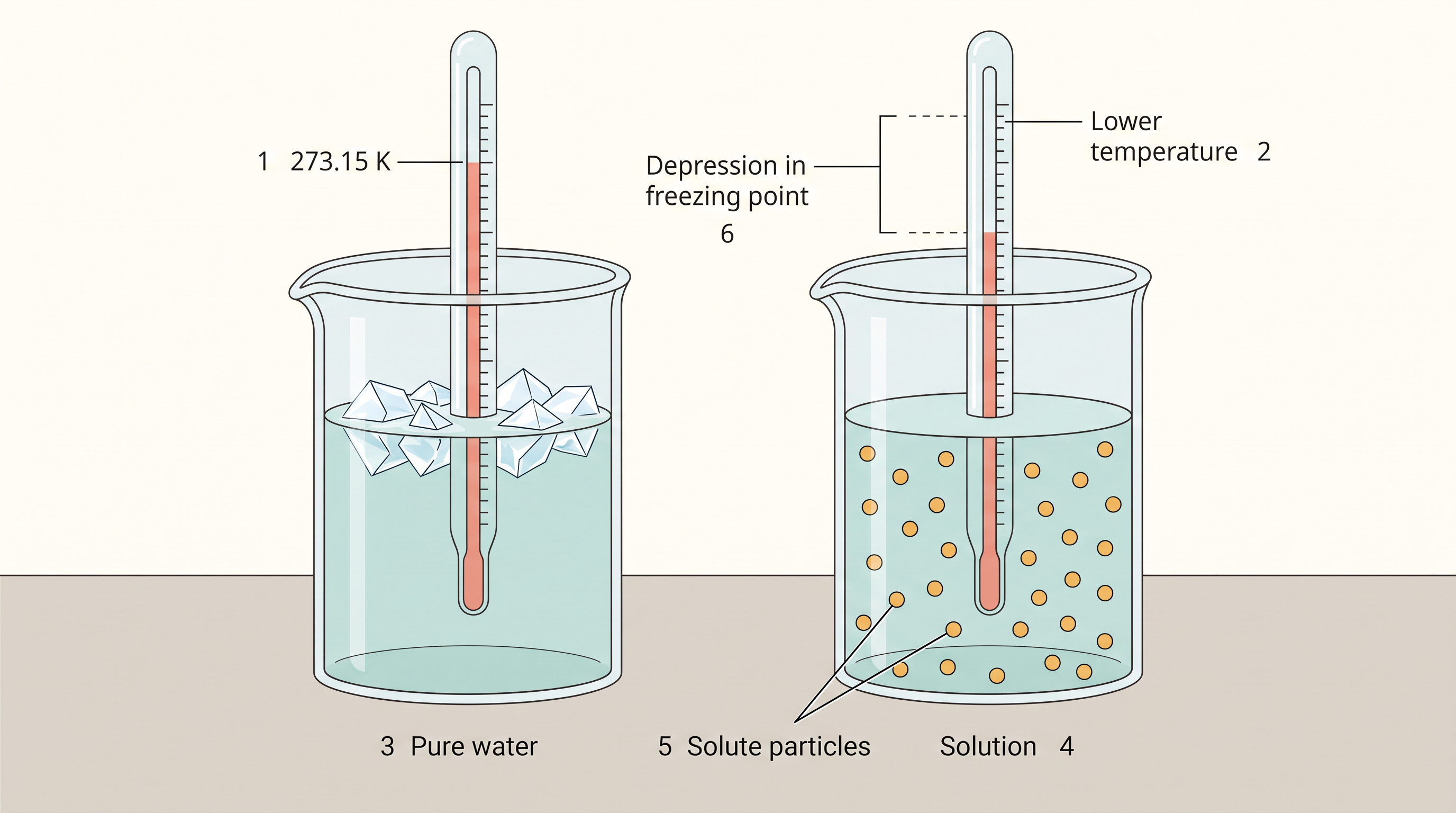
Fig. 1.0 – Depression in the freezing point of a solution.
Keep these questions in mind as you read — this chapter will give you everything you need to reason out each one.
1.1 Types of Solutions
Why Mixtures Matter
In everyday life we rarely handle pure substances. Almost everything around us — the air we breathe, the water we drink, the metal in a doorknob — is a mixture of two or more pure substances. What such a mixture can do for us depends on exactly what it contains and in what proportion.
Consider metals first. Brass is a mixture of copper and zinc, German silver is a mixture of copper, zinc and nickel, and bronze is a mixture of copper and tin. All three are built mainly from copper, yet their hardness, colour and resistance to corrosion are quite different, simply because the other components differ.
The proportion matters just as much as the identity. In drinking water, 1 part per million (ppm) of fluoride ions helps prevent tooth decay, but 1.5 ppm makes the teeth mottled, and a high concentration of fluoride ions is actually poisonous — sodium fluoride, for instance, is used in rat poison. In the same way, an intravenous injection is always dissolved in water containing salts at particular ionic concentrations that match the concentrations in blood plasma, because a mismatch would damage the blood cells.
In this Chapter we shall deal mostly with liquid solutions and how they are formed. We shall then study the properties of solutions, such as vapour pressure and the colligative properties. We begin here with the types of solutions, and then look at the various ways in which the concentration of a solute in a liquid solution can be expressed.
What Exactly Is a Solution?
Solutions are homogeneous mixtures of two or more than two components. By a homogeneous mixture we mean that its composition and its properties are uniform throughout — take a sample from the top of the beaker or from the bottom, and you will find the same composition. This is why a spoonful of sugar solution tastes the same wherever you draw it from.
Generally, the component that is present in the largest quantity is known as the solvent. The solvent decides the physical state in which the solution exists: if the solvent is a liquid, the solution is a liquid, no matter whether the dissolved substance was originally a solid or a gas.
One or more components present in the solution other than the solvent are called solutes. In this Chapter we shall consider only binary solutions, that is, solutions consisting of two components — one solvent and one solute.
The Nine Possible Combinations
In a binary solution each component may be a solid, a liquid or a gas. Since the solute can be in any of these three states and the solvent can also be in any of these three states, there are nine possible types of solution. These are summarised in Table 1.1. Notice that the solutions are grouped by the state of the solvent, because it is the solvent that decides the state of the final solution.
Table 1.1: Types of Solutions
| Type of Solution | Solute | Solvent | Common Examples |
|---|---|---|---|
| Gaseous Solutions | Gas | Gas | Mixture of oxygen and nitrogen gases |
| Liquid | Gas | Chloroform mixed with nitrogen gas | |
| Solid | Gas | Camphor in nitrogen gas | |
| Liquid Solutions | Gas | Liquid | Oxygen dissolved in water |
| Liquid | Liquid | Ethanol dissolved in water | |
| Solid | Liquid | Glucose dissolved in water | |
| Solid Solutions | Gas | Solid | Solution of hydrogen in palladium |
| Liquid | Solid | Amalgam of mercury with sodium | |
| Solid | Solid | Copper dissolved in gold |
The classification is summarised as a scheme in FC 1.1, which is a convenient way to revise the nine cases quickly.
Flowchart
FC 1.1 – Classification of binary solutions by the state of the solvent: Binary solution → branch by solvent state → (Gaseous solvent → gas solute: O₂ + N₂; liquid solute: chloroform in N₂; solid solute: camphor in N₂) → (Liquid solvent → gas solute: O₂ in water; liquid solute: ethanol in water; solid solute: glucose in water) → (Solid solvent → gas solute: H₂ in palladium; liquid solute: sodium amalgam; solid solute: copper in gold). Note at the end: the solvent decides the physical state of the solution.
The alloys mentioned earlier — brass, bronze and German silver — belong to the last row of Table 1.1: they are solid solutions of one metal in another. Air belongs to the first row, and soda water belongs to the row “gas in liquid”, which we shall study in detail when we come to solubility.
1.2 Expressing Concentration of Solutions
The composition of a solution can be described by expressing its concentration. Concentration simply tells us how much solute is present in a given amount of solvent or of solution. It can be expressed either qualitatively or quantitatively.
Qualitatively, we may say that a solution is dilute, meaning that a relatively very small quantity of solute is present, or that it is concentrated, meaning that a relatively very large quantity of solute is present. Such descriptions are convenient in ordinary conversation, but in real work they add a lot of confusion — one chemist’s “dilute” may be another chemist’s “concentrated”. Hence the need for a quantitative description of the solution.
There are several ways by which we can describe the concentration of a solution quantitatively. Each of them compares the amount of one component with the amount of the whole solution (or, in one case, with the amount of solvent alone).
(i) Mass Percentage (w/w)
The mass percentage of a component of a solution is defined as:
\[\text{Mass \% of a component} = \frac{\text{Mass of the component in the solution}}{\text{Total mass of the solution}} \times 100 \qquad (1.1)\]
Notice carefully that the denominator is the mass of the solution, not of the solvent. So if a solution is described as 10% glucose in water by mass, it means that 10 g of glucose is dissolved in 90 g of water, giving a 100 g solution.
Concentration described by mass percentage is commonly used in industrial chemical applications. For example, commercial bleaching solution contains 3.62 mass percentage of sodium hypochlorite in water.
(ii) Volume Percentage (V/V)
The volume percentage is defined as:
\[\text{Volume \% of a component} = \frac{\text{Volume of the component}}{\text{Total volume of solution}} \times 100 \qquad (1.2)\]
For example, a 10% ethanol solution in water means that 10 mL of ethanol is dissolved in water such that the total volume of the solution is 100 mL. Solutions containing liquids are commonly expressed in this unit, because liquids are easier to measure by volume than by mass.
A familiar example is antifreeze. A 35% (\(v/v\)) solution of ethylene glycol is used in cars for cooling the engine. At this concentration the antifreeze lowers the freezing point of water to 255.4 K (–17.6 °C), so the coolant in the radiator does not freeze solid and crack the engine block on a winter night.
(iii) Mass by Volume Percentage (w/V)
Another unit, which is commonly used in medicine and pharmacy, is mass by volume percentage. It is the mass of solute dissolved in 100 mL of the solution. This unit is convenient in a hospital, where a drug is weighed out in grams but delivered to the patient as a measured volume of liquid.
(iv) Parts per Million
When a solute is present in trace quantities — so small that a percentage figure would be a long string of zeros after the decimal point — it is convenient to express concentration in parts per million (ppm), defined as:
\[\text{Parts per million} = \frac{\text{Number of parts of the component}}{\text{Total number of parts of all components of the solution}} \times 10^6 \qquad (1.3)\]
As in the case of percentage, concentration in parts per million can also be expressed as mass to mass, volume to volume and mass to volume. A litre of sea water (which weighs 1030 g) contains about \(6 \times 10^{-3}\) g of dissolved oxygen (\(\mathrm{O_2}\)). Such a small concentration is also expressed as 5.8 g per \(10^6\) g (5.8 ppm) of sea water. The concentration of pollutants in water or in the atmosphere is often expressed in terms of \(\mu\text{g mL}^{-1}\) or ppm.
(v) Mole Fraction
The commonly used symbol for mole fraction is \(x\), and the subscript used on the right hand side of \(x\) denotes the component. It is defined as:
\[\text{Mole fraction of a component} = \frac{\text{Number of moles of the component}}{\text{Total number of moles of all the components}} \qquad (1.4)\]
Recall from Class 11 that the number of moles of a substance is its mass divided by its molar mass. So before you can find a mole fraction, you must always convert the given masses into moles.
For example, in a binary mixture, if the number of moles of A and B are \(n_A\) and \(n_B\) respectively, the mole fraction of A will be
\[x_A = \frac{n_A}{n_A + n_B} \qquad (1.5)\]
For a solution containing \(i\) number of components, we have:
\[x_i = \frac{n_i}{n_1 + n_2 + \ldots\ldots + n_i} = \frac{n_i}{\sum n_i} \qquad (1.6)\]
It can be shown that in a given solution the sum of all the mole fractions is unity, i.e.
\[x_1 + x_2 + \ldots\ldots\ldots\ldots + x_i = 1 \qquad (1.7)\]
Mole fraction is very useful in relating some physical properties of solutions, say vapour pressure, with the concentration of the solution, and is quite useful in describing calculations involving gas mixtures. We shall meet it again in Sections 1.4 and 1.6, where the entire treatment of vapour pressure is built on mole fraction.
(vi) Molarity
Molarity (\(M\)) is defined as the number of moles of solute dissolved in one litre (or one cubic decimetre) of solution,
\[\text{Molarity} = \frac{\text{Moles of solute}}{\text{Volume of solution in litre}} \qquad (1.8)\]
For example, a 0.25 mol L\(^{-1}\) (or 0.25 M) solution of NaOH means that 0.25 mol of NaOH has been dissolved in one litre (or one cubic decimetre) of solution.
(vii) Molality
Molality (\(m\)) is defined as the number of moles of the solute per kilogram (kg) of the solvent and is expressed as:
\[\text{Molality } (m) = \frac{\text{Moles of solute}}{\text{Mass of solvent in kg}} \qquad (1.9)\]
For example, a 1.00 mol kg\(^{-1}\) (or 1.00 m) solution of KCl means that 1 mol (74.5 g) of KCl is dissolved in 1 kg of water.
The single letter that separates molarity from molality is worth guarding: capital M is molarity (per litre of solution), small m is molality (per kilogram of solvent). Mixing them up is one of the commonest ways of losing marks in this chapter.
Which Unit Should You Choose?
Each method of expressing the concentration of a solution has its own merits and demerits. Mass %, ppm, mole fraction and molality are independent of temperature, whereas molarity is a function of temperature. This is because volume depends on temperature and the mass does not — warm a solution and it expands, so the same number of moles now occupies more litres, and the molarity falls slightly, even though nothing has been added or removed.
This is exactly why molality, and not molarity, is used later in the chapter for elevation of boiling point and depression of freezing point: those experiments involve heating and cooling, and a concentration unit that itself changes with temperature would be useless there.
1.3 Solubility
Solubility of a substance is its maximum amount that can be dissolved in a specified amount of solvent at a specified temperature. Notice how carefully this statement is worded: unless we fix the solvent, the amount of solvent and the temperature, the word “solubility” has no definite meaning at all.
Solubility depends upon the nature of the solute and the solvent, as well as on temperature and pressure. Let us consider the effect of these factors in the solution of a solid or of a gas in a liquid.
1.3.1 Solubility of a Solid in a Liquid
Every solid does not dissolve in a given liquid. While sodium chloride and sugar dissolve readily in water, naphthalene and anthracene do not. On the other hand, naphthalene and anthracene dissolve readily in benzene, but sodium chloride and sugar do not.
Why should the same solvent be so welcoming to one solid and so indifferent to another? The pattern that is observed is this: polar solutes dissolve in polar solvents, and non-polar solutes dissolve in non-polar solvents. Water is a polar solvent, its molecules being held together by strong dipole–dipole attractions and hydrogen bonds, and it can pull apart the ions of sodium chloride and surround them. Benzene is non-polar, and it can only mix with molecules held by the weak dispersion forces of the naphthalene type.
In general, a solute dissolves in a solvent if the intermolecular interactions are similar in the two — or, as the working rule of the laboratory puts it, like dissolves like.
Dissolution and Crystallisation
When a solid solute is added to the solvent, some solute dissolves and its concentration increases in solution. This process is known as dissolution.
Meanwhile, some solute particles already in solution collide with the solid solute particles and get separated out of solution. This reverse process is known as crystallisation.
At first, dissolution is much faster than crystallisation, simply because there is very little solute in solution to crystallise back. But as the solution gets richer in solute, crystallisation speeds up. A stage is reached when the two processes occur at the same rate. Under such conditions, the number of solute particles going into solution will be equal to the number of solute particles separating out, and a state of dynamic equilibrium is reached.
\[\text{Solute} + \text{Solvent} \rightleftharpoons \text{Solution} \qquad (1.10)\]
The word dynamic is important. Nothing has stopped at equilibrium; both processes are still going on, but at exactly equal rates, so nothing appears to change. The set-up is easiest to picture as an undissolved layer of solid sitting at the bottom of a beaker while particles constantly leave it and constantly return to it.
At this stage the concentration of solute in solution will remain constant under the given conditions, i.e., temperature and pressure. A similar process is followed when gases are dissolved in liquid solvents.
Saturated and Unsaturated Solutions
Such a solution in which no more solute can be dissolved at the same temperature and pressure is called a saturated solution. An unsaturated solution is one in which more solute can be dissolved at the same temperature.
The solution which is in dynamic equilibrium with undissolved solute is the saturated solution, and it contains the maximum amount of solute dissolved in a given amount of solvent. Thus, the concentration of solute in such a solution is its solubility. This is the link between the two ideas: solubility is nothing but the concentration of a saturated solution.
Earlier we have observed that the solubility of one substance in another depends on the nature of the substances. In addition to these variables, two other parameters, i.e., temperature and pressure, also control this phenomenon.
Effect of Temperature
The solubility of a solid in a liquid is significantly affected by temperature changes. Consider the equilibrium represented by equation (1.10). This, being a dynamic equilibrium, must follow Le Chatelier’s Principle, which you met in Class 11: if a system at equilibrium is disturbed, the equilibrium shifts in the direction that opposes the disturbance. Raising the temperature is a disturbance that the system opposes by favouring whichever direction absorbs heat.
In general, if in a nearly saturated solution the dissolution process is endothermic (\(\Delta_{\text{sol}} H > 0\)), the solubility should increase with rise in temperature; and if it is exothermic (\(\Delta_{\text{sol}} H < 0\)), the solubility should decrease. These trends are also observed experimentally.
Effect of Pressure
Pressure does not have any significant effect on the solubility of solids in liquids. It is so because solids and liquids are highly incompressible and practically remain unaffected by changes in pressure. Squeezing a beaker of salt solution harder does not push the solid particles any closer together, because there is essentially no free space to squeeze out.
Gases, however, are a completely different matter — and that is where we turn next.
1.3.2 Solubility of a Gas in a Liquid
Many gases dissolve in water. Oxygen dissolves only to a small extent in water. It is this dissolved oxygen which sustains all aquatic life — every fish in a river is breathing oxygen that was once in the air above it. On the other hand, hydrogen chloride gas (HCl) is highly soluble in water.
Solubility of gases in liquids is greatly affected by pressure and temperature. The solubility of gases increases with increase of pressure.
Why Pressure Increases Gas Solubility
For a solution of a gas in a solvent, consider a system as shown in Fig. 1.1 (a). The lower part is solution and the upper part is the gaseous system at pressure \(p\) and temperature \(T\). Assume this system to be in a state of dynamic equilibrium, i.e., under these conditions the rate of gaseous particles entering and leaving the solution phase is the same.
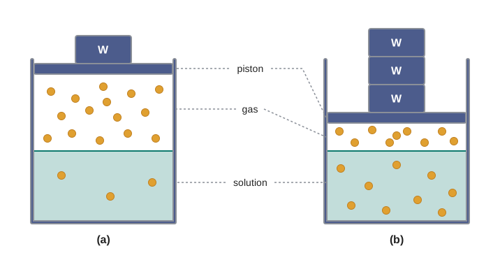
Fig. 1.1 – Effect of pressure on the solubility of a gas.
Now increase the pressure over the solution phase by compressing the gas to a smaller volume [Fig. 1.1 (b)]. This will increase the number of gaseous particles per unit volume over the solution, and also the rate at which the gaseous particles are striking the surface of the solution to enter it. Since more particles are entering the liquid than are leaving it, the solubility of the gas will increase until a new equilibrium is reached — resulting in an increase in the pressure of a gas above the solution, and thus its solubility increases.
Henry’s Law
Henry was the first to give a quantitative relation between pressure and the solubility of a gas in a solvent, which is known as Henry’s law. The law states that at a constant temperature, the solubility of a gas in a liquid is directly proportional to the partial pressure of the gas present above the surface of the liquid or solution.
Dalton, a contemporary of Henry, also concluded independently that the solubility of a gas in a liquid solution is a function of the partial pressure of the gas.
If we use the mole fraction of a gas in the solution as a measure of its solubility, then it can be said that the mole fraction of gas in the solution is proportional to the partial pressure of the gas over the solution. The most commonly used form of Henry’s law states that “the partial pressure of the gas in vapour phase (\(p\)) is proportional to the mole fraction of the gas (\(x\)) in the solution” and is expressed as:
\[p = K_{\mathrm{H}}\,x \qquad (1.11)\]
Here \(K_{\mathrm{H}}\) is the Henry’s law constant.
If we draw a graph between the partial pressure of the gas versus the mole fraction of the gas in solution, then we should get a plot of the type shown in Fig. 1.2 — a straight line through the origin, whose slope is \(K_{\mathrm{H}}\).
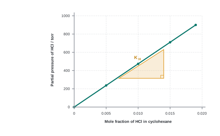
Fig. 1.2 – Solubility of HCl gas in cyclohexane at 293 K.
Different gases have different \(K_{\mathrm{H}}\) values at the same temperature (Table 1.2). This suggests that \(K_{\mathrm{H}}\) is a function of the nature of the gas.
It is obvious from equation (1.11) that the higher the value of \(K_{\mathrm{H}}\) at a given pressure, the lower is the solubility of the gas in the liquid. Read equation (1.11) as \(x = p/K_{\mathrm{H}}\) and this becomes plain — with \(K_{\mathrm{H}}\) in the denominator, a large \(K_{\mathrm{H}}\) means a small mole fraction, that is, a poorly soluble gas.
Table 1.2: Values of Henry’s Law Constant for Some Selected Gases in Water
| Gas | Temperature/K | \(K_{\mathrm{H}}\)/kbar | Gas | Temperature/K | \(K_{\mathrm{H}}\)/kbar |
|---|---|---|---|---|---|
| He | 293 | 144.97 | Argon | 298 | 40.3 |
| \(\mathrm{H_2}\) | 293 | 69.16 | \(\mathrm{CO_2}\) | 298 | 1.67 |
| \(\mathrm{N_2}\) | 293 | 76.48 | Formaldehyde | 298 | \(1.83\times10^{-5}\) |
| \(\mathrm{N_2}\) | 303 | 88.84 | Methane | 298 | 0.413 |
| \(\mathrm{O_2}\) | 293 | 34.86 | Vinyl chloride | 298 | 0.611 |
| \(\mathrm{O_2}\) | 303 | 46.82 |
It can be seen from Table 1.2 that \(K_{\mathrm{H}}\) values for both \(\mathrm{N_2}\) and \(\mathrm{O_2}\) increase with increase of temperature, indicating that the solubility of gases increases with decrease of temperature. It is due to this reason that aquatic species are more comfortable in cold waters rather than in warm waters.
Henry’s Law in Industry and in the Body
Henry’s law finds several applications in industry and explains some biological phenomena. Notable among these are:
To increase the solubility of \(\mathrm{CO_2}\) in soft drinks and soda water, the bottle is sealed under high pressure. A higher partial pressure of \(\mathrm{CO_2}\) above the liquid forces more of it into solution, exactly as equation (1.11) predicts.
Scuba divers must cope with high concentrations of dissolved gases while breathing air at high pressure underwater. Increased pressure increases the solubility of atmospheric gases in blood. When the divers come towards the surface, the pressure gradually decreases. This releases the dissolved gases and leads to the formation of bubbles of nitrogen in the blood. This blocks capillaries and creates a medical condition known as bends, which are painful and dangerous to life.
To avoid bends, as well as the toxic effects of high concentrations of nitrogen in the blood, the tanks used by scuba divers are filled with air diluted with helium (11.7% helium, 56.2% nitrogen and 32.1% oxygen). Look up helium in Table 1.2: its \(K_{\mathrm{H}}\) of 144.97 kbar is the largest in the table, which is precisely why it is chosen — it is the gas least willing to dissolve in blood in the first place.
At high altitudes the partial pressure of oxygen is less than that at the ground level. This leads to low concentrations of oxygen in the blood and tissues of people living at high altitudes or of climbers. Low blood oxygen causes climbers to become weak and unable to think clearly, symptoms of a condition known as anoxia.
The sequence of events that produces the bends is worth fixing in order, as set out in FC 1.2, because the same chain of reasoning — pressure changes, so solubility changes, so dissolved gas must go somewhere — is the key to every Henry’s law application.
Flowchart
FC 1.2 – Why divers get the bends: diver descends → pressure of breathing air rises → partial pressure of N₂ in lungs rises → (Henry’s law) solubility of N₂ in blood rises → extra N₂ dissolves in blood → diver ascends rapidly → pressure falls sharply → blood now holds more N₂ than it can → excess N₂ comes out as bubbles → bubbles block capillaries → bends. Branch: slow, staged ascent → dissolved N₂ is released gradually through the lungs → no bubbles.
Effect of Temperature
The solubility of gases in liquids decreases with rise in temperature. Why should this be so? When dissolved, the gas molecules are present in the liquid phase, and the process of dissolution can be considered similar to condensation — the gas is being “captured” into the liquid — and heat is evolved in this process.
We have learnt in the last Section that the dissolution process involves dynamic equilibrium and thus must follow Le Chatelier’s Principle. As dissolution is an exothermic process, the solubility should decrease with increase of temperature. Heating supplies the very energy that the dissolved molecules need to escape back into the gas phase.
1.4 Vapour Pressure of Liquid Solutions
Liquid solutions are formed when the solvent is a liquid. The solute can be a gas, a liquid or a solid. Solutions of gases in liquids have already been discussed in Section 1.3.2. In this Section, we shall discuss the solutions of liquids and solids in a liquid.
Such solutions may contain one or more volatile components. A volatile substance is simply one that evaporates easily — its molecules escape from the liquid surface into the space above readily at ordinary temperatures. Generally, the liquid solvent is volatile. The solute may or may not be volatile: ethanol dissolved in water is volatile, while sugar dissolved in water is not.
We shall discuss the properties of only binary solutions, that is, the solutions containing two components, namely, the solutions of (i) liquids in liquids and (ii) solids in liquids.
1.4.1 Vapour Pressure of Liquid-Liquid Solutions
Let us consider a binary solution of two volatile liquids and denote the two components as 1 and 2. When taken in a closed vessel, both the components would evaporate, and eventually an equilibrium would be established between the vapour phase and the liquid phase — molecules leaving the liquid surface and molecules returning to it at the same rate.
Let the total vapour pressure at this stage be \(p_{\text{total}}\), and let \(p_1\) and \(p_2\) be the partial vapour pressures of the two components 1 and 2 respectively. These partial pressures are related to the mole fractions \(x_1\) and \(x_2\) of the two components 1 and 2 respectively.
The reason for this relation is easy to picture. Only the molecules sitting at the surface can escape. If component 1 makes up a larger fraction of the molecules in the liquid, it occupies a larger fraction of the surface, so a larger fraction of the escaping molecules are of component 1 — and its contribution to the vapour pressure rises in proportion.
Raoult’s Law for Volatile Liquids
The French chemist, Francois Marte Raoult (1886) gave the quantitative relationship between them. The relationship is known as the Raoult’s law, which states that for a solution of volatile liquids, the partial vapour pressure of each component of the solution is directly proportional to its mole fraction present in solution.
Thus, for component 1
\[p_1 \propto x_1\]
and
\[p_1 = p_1^{0}\,x_1 \qquad (1.12)\]
where \(p_1^{0}\) is the vapour pressure of pure component 1 at the same temperature.
Similarly, for component 2
\[p_2 = p_2^{0}\,x_2 \qquad (1.13)\]
where \(p_2^{0}\) represents the vapour pressure of the pure component 2.
Note carefully what \(p_1^{0}\) means. It is not an arbitrary constant: it is the vapour pressure the component would have if it were present pure, i.e. when \(x_1 = 1\). Raoult’s law therefore says that a component in solution exerts only that fraction of its pure vapour pressure which corresponds to its share of the molecules.
Adding the Two Partial Pressures
According to Dalton’s law of partial pressures, the total pressure (\(p_{\text{total}}\)) over the solution phase in the container will be the sum of the partial pressures of the components of the solution and is given as:
\[p_{\text{total}} = p_1 + p_2 \qquad (1.14)\]
Substituting the values of \(p_1\) and \(p_2\), we get
\[p_{\text{total}} = x_1 p_1^{0} + x_2 p_2^{0}\]
\[= (1 - x_2)\,p_1^{0} + x_2 p_2^{0} \qquad (1.15)\]
\[= p_1^{0} + (p_2^{0} - p_1^{0})\,x_2 \qquad (1.16)\]
The step from (1.15) to (1.16) is only algebra — expand the bracket and collect the terms in \(x_2\) — but it is worth doing carefully, because it puts the equation into the form \(y = c + mx\): a straight line with intercept \(p_1^{0}\) and slope \((p_2^{0} - p_1^{0})\). Here we have used \(x_1 = 1 - x_2\), which is simply equation (1.7) for a binary solution.
The following conclusions can be drawn from equation (1.16).
Total vapour pressure over the solution can be related to the mole fraction of any one component.
Total vapour pressure over the solution varies linearly with the mole fraction of component 2.
Depending on the vapour pressures of the pure components 1 and 2, total vapour pressure over the solution decreases or increases with the increase of the mole fraction of component 1.
A plot of \(p_1\) or \(p_2\) versus the mole fractions \(x_1\) and \(x_2\) for a solution gives a linear plot as shown in Fig. 1.3.
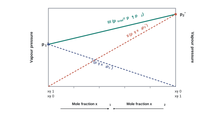
Fig. 1.3 – Vapour pressure of an ideal solution.
These lines (I and II) pass through the points for which \(x_1\) and \(x_2\) are equal to unity — that is, each partial-pressure line ends at the vapour pressure of that pure component. Similarly the plot (line III) of \(p_{\text{total}}\) versus \(x_2\) is also linear (Fig. 1.3). The minimum value of \(p_{\text{total}}\) is \(p_1^{0}\) and the maximum value is \(p_2^{0}\), assuming that component 1 is less volatile than component 2, i.e., \(p_1^{0} < p_2^{0}\).
Composition of the Vapour Phase
The composition of the vapour phase in equilibrium with the solution is determined by the partial pressures of the components. If \(y_1\) and \(y_2\) are the mole fractions of the components 1 and 2 respectively in the vapour phase, then, using Dalton’s law of partial pressures:
\[p_1 = y_1\,p_{\text{total}} \qquad (1.17)\]
\[p_2 = y_2\,p_{\text{total}} \qquad (1.18)\]
In general
\[p_i = y_i\,p_{\text{total}} \qquad (1.19)\]
Keep the two symbols apart: \(x\) always refers to composition in the liquid, and \(y\) always refers to composition in the vapour. They are not equal, and the difference between them is the whole basis of distillation.
1.4.2 Raoult’s Law as a Special Case of Henry’s Law
According to Raoult’s law, the vapour pressure of a volatile component in a given solution is given by \(p_i = x_i\,p_i^{0}\).
In the solution of a gas in a liquid, one of the components is so volatile that it exists as a gas, and we have already seen that its solubility is given by Henry’s law, which states that
\[p = K_{\mathrm{H}}\,x.\]
If we compare the equations for Raoult’s law and Henry’s law, it can be seen that in both cases the partial pressure of the volatile component or gas is directly proportional to its mole fraction in solution. The two equations have exactly the same shape — a pressure equal to a constant times a mole fraction. Only the proportionality constant \(K_{\mathrm{H}}\) differs from \(p_1^{0}\).
Thus, Raoult’s law becomes a special case of Henry’s law, in which \(K_{\mathrm{H}}\) becomes equal to \(p_1^{0}\).
1.4.3 Vapour Pressure of Solutions of Solids in Liquids
Another important class of solutions consists of solids dissolved in liquid — for example, sodium chloride, glucose, urea and cane sugar in water, and iodine and sulphur dissolved in carbon disulphide. Some physical properties of these solutions are quite different from those of pure solvents. Take vapour pressure, for instance.
Liquids at a given temperature vapourise, and under equilibrium conditions the pressure exerted by the vapours of the liquid over the liquid phase is called vapour pressure [Fig. 1.4 (a)].
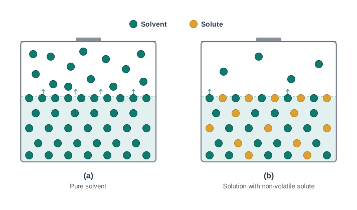
Fig. 1.4 – Lowering of vapour pressure by a non-volatile solute.
Why a Non-Volatile Solute Lowers Vapour Pressure
In a pure liquid the entire surface is occupied by the molecules of the liquid. If a non-volatile solute is added to a solvent to give a solution [Fig. 1.4 (b)], the vapour pressure of the solution is solely from the solvent alone — the solute, being non-volatile, contributes nothing to the vapour.
This vapour pressure of the solution at a given temperature is found to be lower than the vapour pressure of the pure solvent at the same temperature. In the solution, the surface has both solute and solvent molecules; thereby the fraction of the surface covered by the solvent molecules gets reduced. Consequently, the number of solvent molecules escaping from the surface is correspondingly reduced, and thus the vapour pressure is also reduced.
The decrease in the vapour pressure of solvent depends on the quantity of non-volatile solute present in the solution, irrespective of its nature. It is a matter of counting particles, not of identifying them. For example, the decrease in the vapour pressure of water produced by adding 1.0 mol of sucrose to one kg of water is nearly similar to that produced by adding 1.0 mol of urea to the same quantity of water at the same temperature — even though sucrose and urea are completely different substances.
This “counting, not identifying” idea is the seed of the whole of Section 1.6, where such properties are given the name colligative properties.
Raoult’s Law in Its General Form
Raoult’s law in its general form can be stated as: for any solution the partial vapour pressure of each volatile component in the solution is directly proportional to its mole fraction.
In a binary solution, let us denote the solvent by 1 and the solute by 2. When the solute is non-volatile, only the solvent molecules are present in the vapour phase and contribute to the vapour pressure.
Let \(p_1\) be the vapour pressure of the solvent, \(x_1\) be its mole fraction, and \(p_1^{0}\) be its vapour pressure in the pure state. Then according to Raoult’s law
\[p_1 \propto x_1\]
and
\[p_1 = x_1\,p_1^{0} \qquad (1.20)\]
The proportionality constant is equal to the vapour pressure of the pure solvent, \(p_1^{0}\). A plot between the vapour pressure and the mole fraction of the solvent is linear, as shown in Fig. 1.5: it runs from zero (when there is no solvent at all) up to \(p_1^{0}\) (when the solvent is pure, \(x_1 = 1\)).
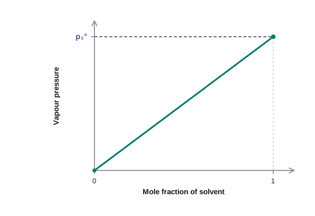
Fig. 1.5 – Vapour pressure versus mole fraction of solvent.
1.5 Ideal and Non-ideal Solutions
Liquid-liquid solutions can be classified into ideal and non-ideal solutions on the basis of Raoult’s law. The test is simple: does the solution actually behave the way equation (1.16) says it should, at every composition — or does it wander away from that prediction?
1.5.1 Ideal Solutions
The solutions which obey Raoult’s law over the entire range of concentration are known as ideal solutions. The words “entire range” matter. A solution that happens to fit Raoult’s law when it is very dilute but drifts away when it is concentrated is not an ideal solution.
The ideal solutions have two other important properties. The enthalpy of mixing of the pure components to form the solution is zero, and the volume of mixing is also zero, i.e.,
\[\Delta_{\text{mix}}H = 0, \qquad \Delta_{\text{mix}}V = 0 \qquad (1.21)\]
It means that no heat is absorbed or evolved when the components are mixed — the mixture neither warms up nor cools down. Also, the volume of the solution would be equal to the sum of the volumes of the two components: mix 50 mL with 50 mL and you get exactly 100 mL, with no shrinking or swelling.
The Molecular Picture
At the molecular level, ideal behaviour of solutions can be explained by considering two components A and B. In the pure components, the intermolecular attractive interactions will be of types A-A and B-B. In the binary solution, in addition to these two interactions, A-B type interactions will also be present.
If the intermolecular attractive forces between the A-A and B-B are nearly equal to those between A-B, this leads to the formation of an ideal solution. In such a mixture, a molecule of A is held in the solution just as firmly as it was held in pure A, so it escapes into the vapour just as easily as before, and Raoult’s law is obeyed exactly.
This also explains the two zeros in equation (1.21). Breaking A-A and B-B contacts costs energy; forming A-B contacts releases energy. If the three kinds of interaction are of equal strength, the cost and the gain cancel, so no heat is absorbed or released and \(\Delta_{\text{mix}}H = 0\). Since the molecules are packing together with the same forces as before, the total volume also stays unchanged, so \(\Delta_{\text{mix}}V = 0\).
A perfectly ideal solution is rare, but some solutions are nearly ideal in behaviour. Solutions of n-hexane and n-heptane, bromoethane and chloroethane, benzene and toluene, etc., fall into this category. Notice what these pairs have in common: in each pair the two molecules are chemically very similar, so A-B forces are naturally about the same as A-A and B-B forces.
1.5.2 Non-ideal Solutions
When a solution does not obey Raoult’s law over the entire range of concentration, then it is called a non-ideal solution. The vapour pressure of such a solution is either higher or lower than that predicted by Raoult’s law (equation 1.16).
If it is higher, the solution exhibits positive deviation, and if it is lower, it exhibits negative deviation from Raoult’s law. The plots of vapour pressure as a function of mole fractions for such solutions are shown in Fig. 1.6, where the dashed straight lines show what Raoult’s law would predict and the curved lines show what is actually measured.
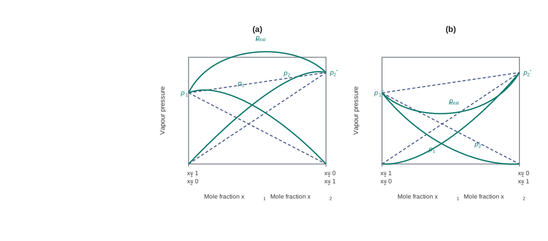
Fig. 1.6 – Deviations from Raoult’s law: (a) positive and (b) negative.
Positive Deviation: Weaker A-B Forces
The cause for these deviations lies in the nature of interactions at the molecular level.
In the case of positive deviation from Raoult’s law, A-B interactions are weaker than those between A-A or B-B. That is, in this case the intermolecular attractive forces between the solute-solvent molecules are weaker than those between the solute-solute and solvent-solvent molecules.
This means that in such solutions, molecules of A (or B) will find it easier to escape than in the pure state. This will increase the vapour pressure and result in positive deviation.
Mixtures of ethanol and acetone behave in this manner. In pure ethanol, the molecules are hydrogen bonded to one another. On adding acetone, its molecules get in between the host molecules and break some of the hydrogen bonds between them. Due to the weakening of interactions, the solution shows positive deviation from Raoult’s law [Fig. 1.6 (a)].
In a solution formed by adding carbon disulphide to acetone, the dipolar interactions between solute-solvent molecules are weaker than the respective interactions among the solute-solute and solvent-solvent molecules. This solution also shows positive deviation.
Since escaping is now easier than it was in the pure liquids, the molecules must have been released from some attraction — and releasing molecules from attraction costs energy. That is why a solution showing positive deviation has \(\Delta_{\text{mix}}H > 0\) (mixing is endothermic) and usually also \(\Delta_{\text{mix}}V > 0\) (the loosely held molecules take up slightly more room).
Negative Deviation: Stronger A-B Forces
In the case of negative deviations from Raoult’s law, the intermolecular attractive forces between A-A and B-B are weaker than those between A-B, and this leads to a decrease in vapour pressure, resulting in negative deviations.
An example of this type is a mixture of phenol and aniline. In this case the intermolecular hydrogen bonding between the phenolic proton and the lone pair on the nitrogen atom of aniline is stronger than the respective intermolecular hydrogen bonding between similar molecules.
Similarly, a mixture of chloroform and acetone forms a solution with negative deviation from Raoult’s law. This is because the chloroform molecule is able to form a hydrogen bond with the acetone molecule, as shown in Fig. 1.7 (c).
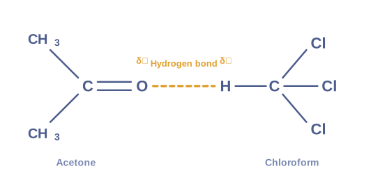
Fig. 1.7 (c) – Hydrogen bonding between acetone and chloroform.
This decreases the escaping tendency of molecules for each component, and consequently the vapour pressure decreases, resulting in negative deviation from Raoult’s law [Fig. 1.6 (b)]. Because a new, stronger attraction is being formed, energy is released on mixing: such solutions have \(\Delta_{\text{mix}}H < 0\) (mixing is exothermic) and usually \(\Delta_{\text{mix}}V < 0\) (the molecules are pulled a little closer together).
Azeotropes
Some liquids on mixing form azeotropes, which are binary mixtures having the same composition in liquid and vapour phase and boiling at a constant temperature.
This is a genuinely awkward situation for a chemist. Fractional distillation works only because the vapour is richer in one component than the liquid it came from (Section 1.4.1). At the azeotropic composition that difference vanishes: the vapour that boils off has exactly the same composition as the liquid left behind, so distilling it changes nothing. In such cases, it is not possible to separate the components by fractional distillation.
There are two types of azeotropes, called minimum boiling azeotrope and maximum boiling azeotrope.
The solutions which show a large positive deviation from Raoult’s law form a minimum boiling azeotrope at a specific composition. Their vapour pressure is abnormally high, so a lower temperature is enough to make that vapour pressure equal atmospheric pressure — hence the low boiling point.
For example, an ethanol-water mixture (obtained by fermentation of sugars) on fractional distillation gives a solution containing approximately 95% by volume of ethanol. Once this composition, known as the azeotrope composition, has been achieved, the liquid and vapour have the same composition, and no further separation occurs.
The solutions that show large negative deviation from Raoult’s law form a maximum boiling azeotrope at a specific composition. Here the vapour pressure is abnormally low, so the mixture must be heated to a higher temperature than either pure liquid before its vapour pressure reaches atmospheric pressure.
Nitric acid and water is an example of this class of azeotrope. This azeotrope has the approximate composition, 68% nitric acid and 32% water by mass, with a boiling point of 393.5 K.
1.6 Colligative Properties and Determination of Molar Mass
We have learnt in Section 1.4.3 that the vapour pressure of a solution decreases when a non-volatile solute is added to a volatile solvent. There are many properties of solutions which are connected with this decrease of vapour pressure. These are:
- relative lowering of vapour pressure of the solvent
- depression of freezing point of the solvent
- elevation of boiling point of the solvent
- osmotic pressure of the solution
All these properties depend on the number of solute particles irrespective of their nature relative to the total number of particles present in the solution. Such properties are called colligative properties (colligative: from Latin — co means together, ligare means to bind).
This “count, don’t identify” idea is what makes the whole section powerful. If a property depends only on the number of dissolved particles, then measuring that property lets us count the particles — and once we can count particles in a weighed sample, we can find the molar mass of the solute. That is why the title of this section joins colligative properties to the determination of molar mass. In the following Sections we will discuss these properties one by one.
1.6.1 Relative Lowering of Vapour Pressure
We have learnt in Section 1.4.3 that the vapour pressure of a solvent in solution is less than that of the pure solvent. Raoult established that the lowering of vapour pressure depends only on the concentration of the solute particles and it is independent of their identity.
The equation (1.20) given in Section 1.4.3 establishes a relation between the vapour pressure of the solution, the mole fraction and the vapour pressure of the solvent, i.e.,
\[p_1 = x_1\,p_1^{0} \qquad (1.22)\]
The reduction in the vapour pressure of solvent (\(\Delta p_1\)) is given as:
\[\Delta p_1 = p_1^{0} - p_1 = p_1^{0} - p_1^{0}x_1\]
\[= p_1^{0}\,(1 - x_1) \qquad (1.23)\]
Knowing that \(x_2 = 1 - x_1\), equation (1.23) reduces to
\[\Delta p_1 = x_2\,p_1^{0} \qquad (1.24)\]
Read equation (1.24) slowly: the drop in vapour pressure is fixed by \(x_2\), the mole fraction of the solute — not by what the solute is.
In a solution containing several non-volatile solutes, the lowering of the vapour pressure depends on the sum of the mole fractions of the different solutes.
Equation (1.24) can be written as
\[\frac{\Delta p_1}{p_1^{0}} = \frac{p_1^{0} - p_1}{p_1^{0}} = x_2 \qquad (1.25)\]
The expression on the left hand side of the equation as mentioned earlier is called relative lowering of vapour pressure and is equal to the mole fraction of the solute.
The above equation can be written as:
\[\frac{p_1^{0} - p_1}{p_1^{0}} = \frac{n_2}{n_1 + n_2} \qquad \left(\text{since } x_2 = \frac{n_2}{n_1 + n_2}\right) \qquad (1.26)\]
Here \(n_1\) and \(n_2\) are the number of moles of solvent and solute respectively present in the solution.
For dilute solutions \(n_2 << n_1\), hence neglecting \(n_2\) in the denominator we have
\[\frac{p_1^{0} - p_1}{p_1^{0}} = \frac{n_2}{n_1} \qquad (1.27)\]
This approximation is allowed only because the solution is dilute: the few moles of solute make almost no difference to the total. It is the same approximation we used in Example 1.6 for a dissolved gas.
or
\[\frac{p_1^{0} - p_1}{p_1^{0}} = \frac{w_2 \times M_1}{M_2 \times w_1} \qquad (1.28)\]
Here \(w_1\) and \(w_2\) are the masses and \(M_1\) and \(M_2\) are the molar masses of the solvent and solute respectively. Equation (1.28) simply follows from (1.27) by writing each number of moles as mass divided by molar mass: \(n_2 = w_2/M_2\) and \(n_1 = w_1/M_1\).
From this equation (1.28), knowing all other quantities, the molar mass of solute (\(M_2\)) can be calculated. This is the first of our four molar-mass “weighing machines”.
1.6.2 Elevation of Boiling Point
The vapour pressure of a liquid increases with increase of temperature. It boils at the temperature at which its vapour pressure is equal to the atmospheric pressure. For example, water boils at 373.15 K (100 °C) because at this temperature the vapour pressure of water is 1.013 bar (1 atmosphere).
We have also learnt in the last section that the vapour pressure of the solvent decreases in the presence of a non-volatile solute. Fig. 1.8 depicts the variation of vapour pressure of the pure solvent and of the solution as a function of temperature — the curve for the solution lies below the curve for the pure solvent at every temperature.
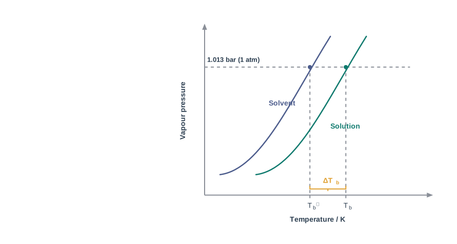
Fig. 1.8 – Elevation of boiling point.
For example, the vapour pressure of an aqueous solution of sucrose is less than 1.013 bar at 373.15 K. In order to make this solution boil, its vapour pressure must be increased to 1.013 bar by raising the temperature above the boiling temperature of the pure solvent (water).
Thus, the boiling point of a solution is always higher than that of the boiling point of the pure solvent in which the solution is prepared, as shown in Fig. 1.8.
Similar to the lowering of vapour pressure, the elevation of boiling point also depends on the number of solute molecules rather than their nature. A solution of 1 mol of sucrose in 1000 g of water boils at 373.52 K at one atmospheric pressure.
Let \(T_{\mathrm{b}}^{0}\) be the boiling point of pure solvent and \(T_{\mathrm{b}}\) be the boiling point of the solution. The increase in the boiling point \(\Delta T_{\mathrm{b}} = T_{\mathrm{b}} - T_{\mathrm{b}}^{0}\) is known as elevation of boiling point.
The Working Equation
Experiments have shown that for dilute solutions the elevation of boiling point (\(\Delta T_{\mathrm{b}}\)) is directly proportional to the molal concentration of the solute in a solution. Thus
\[\Delta T_{\mathrm{b}} \propto m \qquad (1.29)\]
or
\[\Delta T_{\mathrm{b}} = K_{\mathrm{b}}\,m \qquad (1.30)\]
Here \(m\) (molality) is the number of moles of solute dissolved in 1 kg of solvent, and the constant of proportionality, \(K_{\mathrm{b}}\), is called Boiling Point Elevation Constant or Molal Elevation Constant (Ebullioscopic Constant).
The unit of \(K_{\mathrm{b}}\) is K kg mol\(^{-1}\). Values of \(K_{\mathrm{b}}\) for some common solvents are given in Table 1.3. Notice that molality — and not molarity — is used here, for the reason given in Section 1.2: this is an experiment involving heating, and molality does not change with temperature.
If \(w_2\) gram of solute of molar mass \(M_2\) is dissolved in \(w_1\) gram of solvent, then molality, \(m\), of the solution is given by the expression:
\[m = \frac{w_2/M_2}{w_1/1000} = \frac{1000 \times w_2}{M_2 \times w_1} \qquad (1.31)\]
The factor of 1000 appears only because \(w_1\) is in grams while molality demands kilograms of solvent.
Substituting the value of molality in equation (1.30) we get
\[\Delta T_{\mathrm{b}} = \frac{K_{\mathrm{b}} \times 1000 \times w_2}{M_2 \times w_1} \qquad (1.32)\]
Rearranging to make \(M_2\) the subject,
\[M_2 = \frac{1000 \times w_2 \times K_{\mathrm{b}}}{\Delta T_{\mathrm{b}} \times w_1} \qquad (1.33)\]
Thus, in order to determine \(M_2\), the molar mass of the solute, a known mass of solute in a known mass of the solvent is taken, and \(\Delta T_{\mathrm{b}}\) is determined experimentally for a known solvent whose \(K_{\mathrm{b}}\) value is known.
1.6.3 Depression of Freezing Point
The lowering of vapour pressure of a solution causes a lowering of the freezing point compared to that of the pure solvent (Fig. 1.9).
We know that at the freezing point of a substance, the solid phase is in dynamic equilibrium with the liquid phase. Thus, the freezing point of a substance may be defined as the temperature at which the vapour pressure of the substance in its liquid phase is equal to its vapour pressure in the solid phase.
A solution will freeze when its vapour pressure equals the vapour pressure of the pure solid solvent, as is clear from Fig. 1.9. It is important to realise that the solid that separates out on freezing is pure solvent (pure ice, in the case of an aqueous solution), so the relevant solid curve is that of the pure solvent.
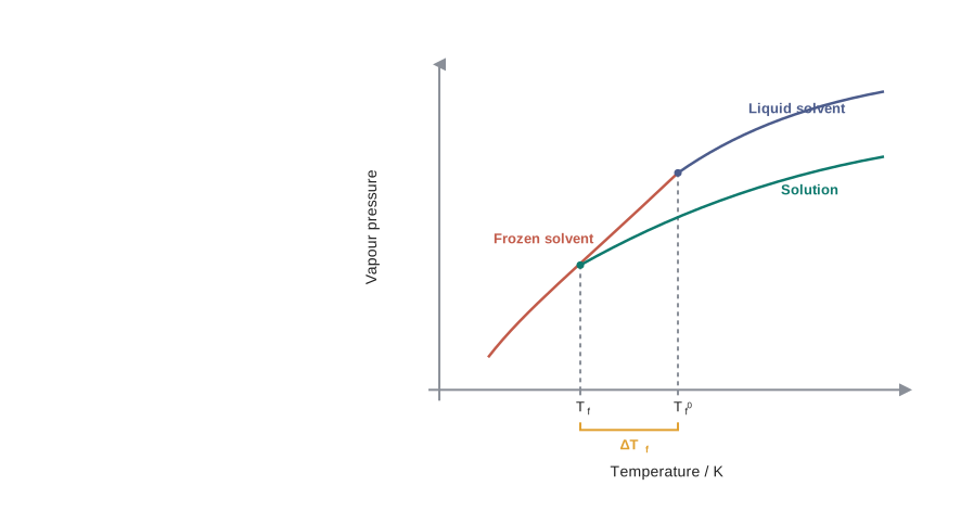
Fig. 1.9 – Depression of freezing point.
According to Raoult’s law, when a non-volatile solid is added to the solvent, its vapour pressure decreases, and now it would become equal to that of the solid solvent at a lower temperature. Thus, the freezing point of the solvent decreases.
Let \(T_{\mathrm{f}}^{0}\) be the freezing point of pure solvent and \(T_{\mathrm{f}}\) be its freezing point when a non-volatile solute is dissolved in it. The decrease in freezing point
\[\Delta T_{\mathrm{f}} = T_{\mathrm{f}}^{0} - T_{\mathrm{f}}\]
is known as depression in freezing point. Note the order of the two terms carefully: it is the reverse of the order used for \(\Delta T_{\mathrm{b}}\), and it is written that way so that \(\Delta T_{\mathrm{f}}\) also comes out positive.
The Working Equation
Similar to the elevation of boiling point, the depression of freezing point (\(\Delta T_{\mathrm{f}}\)) for a dilute solution (ideal solution) is directly proportional to the molality, \(m\), of the solution. Thus,
\[\Delta T_{\mathrm{f}} \propto m\]
or
\[\Delta T_{\mathrm{f}} = K_{\mathrm{f}}\,m \qquad (1.34)\]
The proportionality constant, \(K_{\mathrm{f}}\), which depends on the nature of the solvent, is known as Freezing Point Depression Constant or Molal Depression Constant or Cryoscopic Constant. The unit of \(K_{\mathrm{f}}\) is K kg mol\(^{-1}\). Values of \(K_{\mathrm{f}}\) for some common solvents are listed in Table 1.3.
If \(w_2\) gram of the solute having molar mass as \(M_2\), present in \(w_1\) gram of solvent, produces the depression in freezing point \(\Delta T_{\mathrm{f}}\) of the solvent, then the molality of the solute is given by the equation (1.31).
\[m = \frac{w_2/M_2}{w_1/1000} \qquad (1.31)\]
Substituting this value of molality in equation (1.34) we get:
\[\Delta T_{\mathrm{f}} = \frac{K_{\mathrm{f}} \times w_2/M_2}{w_1/1000}\]
\[\Delta T_{\mathrm{f}} = \frac{K_{\mathrm{f}} \times w_2 \times 1000}{M_2 \times w_1} \qquad (1.35)\]
\[M_2 = \frac{K_{\mathrm{f}} \times w_2 \times 1000}{\Delta T_{\mathrm{f}} \times w_1} \qquad (1.36)\]
Thus, for determining the molar mass of the solute we should know the quantities \(w_1\), \(w_2\), \(\Delta T_{\mathrm{f}}\), along with the molal freezing point depression constant.
Where \(K_{\mathrm{f}}\) and \(K_{\mathrm{b}}\) Come From
The values of \(K_{\mathrm{f}}\) and \(K_{\mathrm{b}}\), which depend upon the nature of the solvent, can be ascertained from the following relations.
\[K_{\mathrm{f}} = \frac{R \times M_1 \times T_{\mathrm{f}}^{2}}{1000 \times \Delta_{\text{fus}}H} \qquad (1.37)\]
\[K_{\mathrm{b}} = \frac{R \times M_1 \times T_{\mathrm{b}}^{2}}{1000 \times \Delta_{\text{vap}}H} \qquad (1.38)\]
Here the symbols \(R\) and \(M_1\) stand for the gas constant and the molar mass of the solvent, respectively, and \(T_{\mathrm{f}}\) and \(T_{\mathrm{b}}\) denote the freezing point and the boiling point of the pure solvent respectively in kelvin. Further, \(\Delta_{\text{fus}}H\) and \(\Delta_{\text{vap}}H\) represent the enthalpies for the fusion and vapourisation of the solvent, respectively.
These two equations confirm in symbols what the tables show in numbers: \(K_{\mathrm{f}}\) and \(K_{\mathrm{b}}\) contain nothing whatever about the solute. Every quantity on the right-hand side belongs to the solvent.
Table 1.3: Molal Boiling Point Elevation and Freezing Point Depression Constants for Some Solvents
| Solvent | b. p./K | \(K_{\mathrm{b}}\)/K kg mol\(^{-1}\) | f. p./K | \(K_{\mathrm{f}}\)/K kg mol\(^{-1}\) |
|---|---|---|---|---|
| Water | 373.15 | 0.52 | 273.0 | 1.86 |
| Ethanol | 351.5 | 1.20 | 155.7 | 1.99 |
| Cyclohexane | 353.74 | 2.79 | 279.55 | 20.00 |
| Benzene | 353.3 | 2.53 | 278.6 | 5.12 |
| Chloroform | 334.4 | 3.63 | 209.6 | 4.79 |
| Carbon tetrachloride | 350.0 | 5.03 | 250.5 | 31.8 |
| Carbon disulphide | 319.4 | 2.34 | 164.2 | 3.83 |
| Diethyl ether | 307.8 | 2.02 | 156.9 | 1.79 |
| Acetic acid | 391.1 | 2.93 | 290.0 | 3.90 |
1.6.4 Osmosis and Osmotic Pressure
There are many phenomena which we observe in nature or at home. For example, raw mangoes shrivel when pickled in brine (salt water); wilted flowers revive when placed in fresh water; blood cells collapse when suspended in saline water, and so on.
If we look into these processes we find one thing common in all — that is, all these substances are bound by membranes. These membranes can be of animal or vegetable origin, and these occur naturally, such as pig’s bladder or parchment, or can be synthetic, such as cellophane.
These membranes appear to be continuous sheets or films, yet they contain a network of submicroscopic holes or pores. Small solvent molecules, like water, can pass through these holes, but the passage of bigger molecules like solute is hindered. Membranes having this kind of properties are known as semipermeable membranes (SPM).
Osmosis
Assume that only solvent molecules can pass through these semipermeable membranes. If this membrane is placed between the solvent and the solution as shown in Fig. 1.10, the solvent molecules will flow through the membrane from pure solvent to the solution. This process of flow of the solvent is called osmosis.
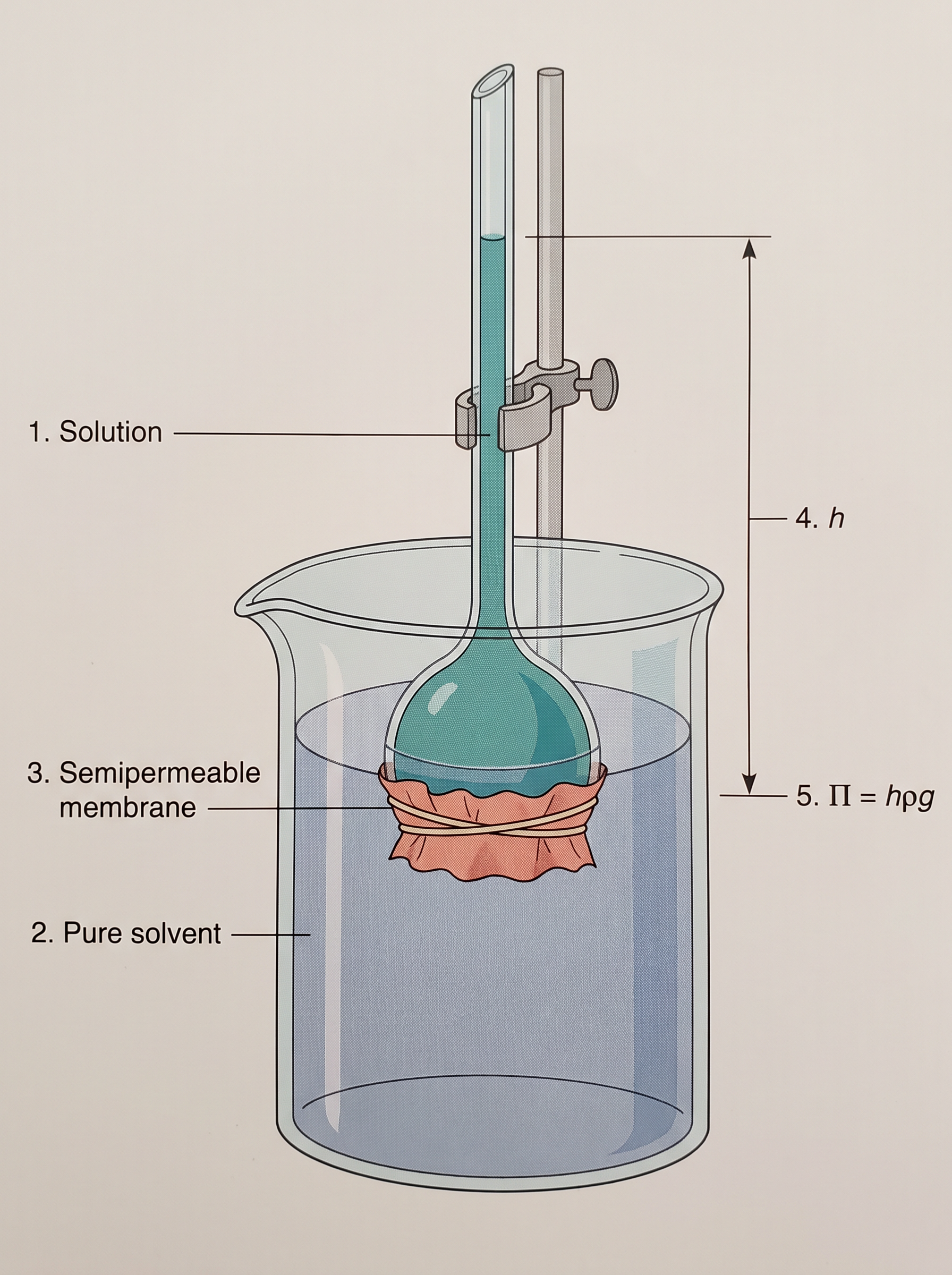
Fig. 1.10 – Osmosis in a thistle funnel.
The flow will continue till equilibrium is attained. As solvent enters the solution in Fig. 1.10, the liquid column rises, and the extra weight of that column presses down on the solution — until the pressure it exerts is just enough to stop any further net flow.
The flow of the solvent from its side to the solution side across a semipermeable membrane can be stopped if some extra pressure is applied on the solution. This pressure that just stops the flow of solvent is called osmotic pressure of the solution.
The flow of solvent from a dilute solution to the concentrated solution across a semipermeable membrane is due to osmosis. The important point to be kept in mind is that solvent molecules always flow from lower concentration to higher concentration of solution. The osmotic pressure has been found to depend on the concentration of the solution.
The osmotic pressure of a solution is the excess pressure that must be applied to a solution to prevent osmosis, i.e., to stop the passage of solvent molecules through a semipermeable membrane into the solution. This is illustrated in Fig. 1.11.
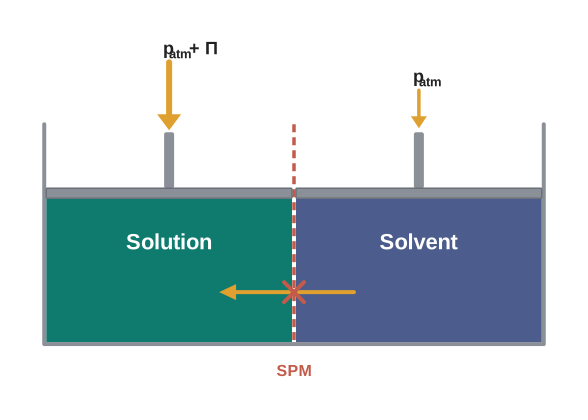
Fig. 1.11 – Osmotic pressure stops the flow of solvent.
The Osmotic Pressure Equation
Osmotic pressure is a colligative property, as it depends on the number of solute molecules and not on their identity.
For dilute solutions, it has been found experimentally that osmotic pressure is proportional to the molarity, \(C\), of the solution at a given temperature \(T\). Thus:
\[\Pi = C\,R\,T \qquad (1.39)\]
Here \(\Pi\) is the osmotic pressure and \(R\) is the gas constant. The resemblance of this equation to the ideal gas equation \(PV = nRT\) is striking, and not accidental: dissolved particles roaming through a solvent behave in many ways like gas particles roaming through a container.
\[\Pi = (n_2/V)\,R\,T \qquad (1.40)\]
Here \(V\) is the volume of a solution in litres containing \(n_2\) moles of solute. If \(w_2\) grams of solute, of molar mass \(M_2\), is present in the solution, then \(n_2 = w_2/M_2\) and we can write,
\[\Pi\,V = \frac{w_2\,R\,T}{M_2} \qquad (1.41)\]
or
\[M_2 = \frac{w_2\,R\,T}{\Pi\,V} \qquad (1.42)\]
Thus, knowing the quantities \(w_2\), \(T\), \(\Pi\) and \(V\) we can calculate the molar mass of the solute.
Measurement of osmotic pressure provides another method of determining the molar masses of solutes. This method is widely used to determine molar masses of proteins, polymers and other macromolecules.
The osmotic pressure method has the advantage over other methods, as pressure measurement is done around room temperature and the molarity of the solution is used instead of molality. As compared to other colligative properties, its magnitude is large even for very dilute solutions — which is exactly what a chemist needs when the solute is a protein of enormous molar mass and only a milligram of it is available.
The technique of osmotic pressure for the determination of molar mass of solutes is particularly useful for biomolecules, as they are generally not stable at higher temperatures — a boiling-point experiment would simply destroy them — and polymers have poor solubility, so only very dilute solutions can be made in the first place.
Isotonic, Hypertonic and Hypotonic Solutions
Two solutions having the same osmotic pressure at a given temperature are called isotonic solutions. When such solutions are separated by a semipermeable membrane, no osmosis occurs between them — neither side is “pulling” harder than the other.
For example, the osmotic pressure associated with the fluid inside the blood cell is equivalent to that of 0.9% (mass/volume) sodium chloride solution, called normal saline solution, and it is safe to inject intravenously.
On the other hand, if we place the cells in a solution containing more than 0.9% (mass/volume) sodium chloride, water will flow out of the cells and they would shrink. Such a solution is called hypertonic.
If the salt concentration is less than 0.9% (mass/volume), the solution is said to be hypotonic. In this case, water will flow into the cells if placed in this solution and they would swell.
Osmosis in Everyday Life
The phenomena mentioned at the beginning of this section can be explained on the basis of osmosis.
A raw mango placed in concentrated salt solution loses water via osmosis and shrivels into pickle. Wilted flowers revive when placed in fresh water. A carrot that has become limp because of water loss into the atmosphere can be placed into water, making it firm once again — water will move into its cells through osmosis.
When placed in water containing less than 0.9% (mass/volume) salt, blood cells swell due to the flow of water into them by osmosis.
People taking a lot of salt or salty food experience water retention in tissue cells and intercellular spaces because of osmosis. The resulting puffiness or swelling is called edema.
Water movement from soil into plant roots, and subsequently into the upper portion of the plant, is partly due to osmosis.
The preservation of meat by salting and of fruits by adding sugar protects against bacterial action. Through the process of osmosis, a bacterium on salted meat or candied fruit loses water, shrivels and dies. This is one of the oldest food-preservation techniques known, and it is pure colligative chemistry: the salt or sugar makes the surroundings hypertonic to the microorganism.
1.6.5 Reverse Osmosis and Water Purification
The direction of osmosis can be reversed if a pressure larger than the osmotic pressure is applied to the solution side. That is, now the pure solvent flows out of the solution through the semipermeable membrane. This phenomenon is called reverse osmosis and is of great practical utility.
Reverse osmosis is used in desalination of sea water. A schematic set-up for the process is shown in Fig. 1.12.
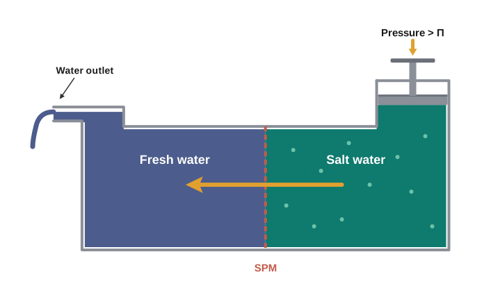
Fig. 1.12 – Reverse osmosis.
When pressure more than the osmotic pressure is applied, pure water is squeezed out of the sea water through the membrane. A variety of polymer membranes are available for this purpose.
The pressure required for reverse osmosis is quite high — which stands to reason, since sea water is a concentrated solution and therefore has a large osmotic pressure that must first be overcome before anything at all happens.
A workable porous membrane is a film of cellulose acetate placed over a suitable support. Cellulose acetate is permeable to water but impermeable to the impurities and ions present in sea water. These days many countries use desalination plants to meet their potable water requirements.
1.7 Abnormal Molar Masses
Every molar mass we calculated in Section 1.6 rested on one quiet assumption: that each formula unit we dissolved gave exactly one particle in solution. For many solutes that is simply not true — and when it is not true, the molar mass that comes out of a colligative-property experiment is wrong. Such a value is called an abnormal molar mass, and this section explains where it comes from and how to correct for it.
When the Solute Breaks Apart
We know that ionic compounds, when dissolved in water, dissociate into cations and anions. For example, if we dissolve one mole of KCl (74.5 g) in water, we expect one mole each of \(\mathrm{K^{+}}\) and \(\mathrm{Cl^{-}}\) ions to be released in the solution. If this happens, there would be two moles of particles in the solution.
If we ignore interionic attractions, one mole of KCl in one kg of water would be expected to increase the boiling point by 2 × 0.52 K = 1.04 K — twice the elevation that one mole of a non-electrolyte such as glucose would produce, because a colligative property counts particles.
Now, if we did not know about the degree of dissociation, we could be led to conclude that the mass of 2 mol of particles is 74.5 g, and hence that the mass of one mole of KCl would be 37.25 g — exactly half of the true value. This brings to light the rule that, when there is dissociation of solute into ions, the experimentally determined molar mass is always lower than the true value.
When the Solute Sticks Together
The opposite can also happen. Molecules of ethanoic acid (acetic acid) dimerise in benzene due to hydrogen bonding. This normally happens in solvents of low dielectric constant, which are unable to pull the polar molecules apart. In this case the number of particles is reduced due to dimerisation.
The association of molecules is depicted as follows:
\[2\,\mathrm{CH_3COOH} \rightleftharpoons (\mathrm{CH_3COOH})_2\]
The two acid molecules lock on to each other through a pair of hydrogen bonds between the –OH of one and the C=O of the other, forming a closed ring, as shown in Fig. 1.13.
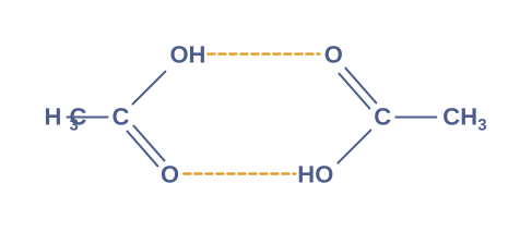
Fig. 1.13 – The cyclic dimer of ethanoic acid.
It can be undoubtedly stated here that if all the molecules of ethanoic acid associate in benzene, then \(\Delta T_{\mathrm{b}}\) or \(\Delta T_{\mathrm{f}}\) for ethanoic acid will be half of the normal value — because two molecules now behave as a single particle. The molar mass calculated on the basis of this \(\Delta T_{\mathrm{b}}\) or \(\Delta T_{\mathrm{f}}\) will, therefore, be twice the expected value: look back at equation (1.36), where \(\Delta T_{\mathrm{f}}\) sits in the denominator, and halving it must double \(M_2\).
Such a molar mass that is either lower or higher than the expected or normal value is called an abnormal molar mass.
The van’t Hoff Factor
In 1880 van’t Hoff introduced a factor \(i\), known as the van’t Hoff factor, to account for the extent of dissociation or association. This factor \(i\) is defined as:
\[i = \frac{\text{Normal molar mass}}{\text{Abnormal molar mass}}\]
\[= \frac{\text{Observed colligative property}}{\text{Calculated colligative property}}\]
\[i = \frac{\text{Total number of moles of particles after association/dissociation}}{\text{Number of moles of particles before association/dissociation}}\]
All three expressions say the same thing in different currencies: \(i\) is simply the factor by which the number of particles has changed.
Here the abnormal molar mass is the experimentally determined molar mass, and the calculated colligative properties are obtained by assuming that the non-volatile solute is neither associated nor dissociated.
In case of association, the value of \(i\) is less than unity, while for dissociation it is greater than unity. For example, the value of \(i\) for aqueous KCl solution is close to 2, while the value for ethanoic acid in benzene is nearly 0.5.
Corrected Colligative-Property Equations
Inclusion of the van’t Hoff factor modifies the equations for colligative properties as follows:
Relative lowering of vapour pressure of solvent,
\[\frac{p_1^{o} - p_1}{p_1^{o}} = i\,.\,\frac{n_2}{n_1}\]
Elevation of Boiling point,
\[\Delta T_b = i\,K_b\,m\]
Depression of Freezing point,
\[\Delta T_f = i\,K_f\,m\]
Osmotic pressure of solution,
\[\Pi = i\,n_2\,R\,T\,/\,V\]
In every case \(i\) enters as a simple multiplier, which is exactly what you would expect: it is correcting the count of particles, and the colligative property is proportional to that count.
Table 1.4: Values of van’t Hoff factor, \(i\), at Various Concentrations for NaCl, KCl, \(\mathrm{MgSO_4}\) and \(\mathrm{K_2SO_4}\).
| Salt | *Values of \(i\): 0.1 m | 0.01 m | 0.001 m | van’t Hoff Factor \(i\) for complete dissociation of solute |
|---|---|---|---|---|
| NaCl | 1.87 | 1.94 | 1.97 | 2.00 |
| KCl | 1.85 | 1.94 | 1.98 | 2.00 |
| \(\mathrm{MgSO_4}\) | 1.21 | 1.53 | 1.82 | 2.00 |
| \(\mathrm{K_2SO_4}\) | 2.32 | 2.70 | 2.84 | 3.00 |
* represent \(i\) values for incomplete dissociation.
Table 1.4 depicts values of the factor, \(i\), for several strong electrolytes. For KCl, NaCl and \(\mathrm{MgSO_4}\), \(i\) values approach 2 as the solution becomes very dilute. As expected, the value of \(i\) gets close to 3 for \(\mathrm{K_2SO_4}\), since one formula unit of \(\mathrm{K_2SO_4}\) can give three ions — two \(\mathrm{K^{+}}\) and one \(\mathrm{SO_4^{2-}}\).
1.8 Summary
What a solution is
- A solution is a homogeneous mixture of two or more substances. The component present in the largest amount is the solvent; the rest are solutes. Solutions are classified as solid, liquid or gaseous, according to the state of the solvent.
Expressing concentration
- The concentration of a solution is expressed in terms of mole fraction, molarity, molality and in percentages (mass %, volume %, mass by volume %, and ppm for trace amounts).
- Mass %, ppm, mole fraction and molality do not change with temperature; molarity does, because volume changes with temperature.
Solubility of a gas: Henry’s law
- The dissolution of a gas in a liquid is governed by Henry’s law, according to which, at a given temperature, the solubility of a gas in a liquid is directly proportional to the partial pressure of the gas.
\[p = K_H\,x\]
- A larger \(K_H\) means a lower solubility. The solubility of a gas falls as the temperature rises, because dissolution of a gas is exothermic.
Vapour pressure: Raoult’s law
- The vapour pressure of the solvent is lowered by the presence of a non-volatile solute in the solution. This lowering is governed by Raoult’s law, according to which the relative lowering of vapour pressure of the solvent over a solution is equal to the mole fraction of a non-volatile solute present in the solution.
\[\frac{p_1^0 - p_1}{p_1^0} = x_2\]
- However, in a binary liquid solution, if both the components of the solution are volatile, then another form of Raoult’s law is used. Mathematically, this form of Raoult’s law is stated as:
\[p_{\text{total}} = p_1^0 x_1 + p_2^0 x_2\]
- At equilibrium, the vapour phase is always richer in the more volatile component — which is what makes distillation possible.
Ideal and non-ideal solutions
- Solutions which obey Raoult’s law over the entire range of concentration are called ideal solutions. For them, \(\Delta_{\text{mix}}H = 0\) and \(\Delta_{\text{mix}}V = 0\).
- Two types of deviations from Raoult’s law, called positive and negative deviations, are observed. Positive deviation arises when A–B attractions are weaker than A–A and B–B attractions; negative deviation arises when A–B attractions are stronger.
- Azeotropes arise due to very large deviations from Raoult’s law. A large positive deviation gives a minimum boiling azeotrope, a large negative deviation a maximum boiling azeotrope. An azeotrope has the same composition in the liquid and vapour phases, so its components cannot be separated by fractional distillation.
Colligative properties
- The properties of solutions which depend on the number of solute particles and are independent of their chemical identity are called colligative properties. These are lowering of vapour pressure, elevation of boiling point, depression of freezing point and osmotic pressure.
\[\Delta T_b = K_b\,m, \qquad \Delta T_f = K_f\,m, \qquad \Pi = C R T\]
- The process of osmosis can be reversed if a pressure higher than the osmotic pressure is applied to the solution. This reverse osmosis is used in the desalination of sea water.
- Colligative properties have been used to determine the molar mass of solutes. Solutes which dissociate in solution exhibit a molar mass lower than the actual molar mass, and those which associate show a higher molar mass than their actual values.
van’t Hoff factor
- Quantitatively, the extent to which a solute is dissociated or associated can be expressed by the van’t Hoff factor \(i\). This factor has been defined as the ratio of normal molar mass to experimentally determined molar mass, or as the ratio of the observed colligative property to the calculated colligative property.
- \(i > 1\) indicates dissociation, \(i < 1\) indicates association, and \(i = 1\) means the solute neither dissociates nor associates. Including \(i\) corrects each colligative-property equation, for example \(\Delta T_f = i\,K_f\,m\) and \(\Pi = i\,n_2 R T / V\).
The chain of reasoning of this chapter
The whole chapter hangs together as one line of argument, which is worth revising as a single sequence, shown in FC 1.4.
Flowchart
FC 1.4 – The logic of the chapter: non-volatile solute added to solvent → solute particles occupy part of the surface → fewer solvent molecules escape → vapour pressure of solvent is lowered (Raoult’s law) → branch 1: solution must be heated higher to reach 1 atm → elevation of boiling point (ΔT_b = K_b m); branch 2: solution’s vapour pressure equals that of the solid only at a lower temperature → depression of freezing point (ΔT_f = K_f m); branch 3: solvent flows through a semipermeable membrane into the solution → osmosis → osmotic pressure (Π = CRT). All three branches → each depends only on the NUMBER of solute particles → colligative properties → used to find molar mass M₂ → if the solute dissociates or associates, correct with the van’t Hoff factor i → true molar mass.
1.9 NCERT Questions
Define the term solution. How many types of solutions are formed? Write briefly about each type with an example.
Give an example of a solid solution in which the solute is a gas.
Define the following terms: (i) Mole fraction (ii) Molality (iii) Molarity (iv) Mass percentage.
Concentrated nitric acid used in laboratory work is 68% nitric acid by mass in aqueous solution. What should be the molarity of such a sample of the acid if the density of the solution is 1.504 g mL\(^{-1}\)?
A solution of glucose in water is labelled as 10% w/w. What would be the molality and mole fraction of each component in the solution? If the density of the solution is 1.2 g mL\(^{-1}\), then what shall be the molarity of the solution?
How many mL of 0.1 M HCl are required to react completely with 1 g mixture of \(\mathrm{Na_2CO_3}\) and \(\mathrm{NaHCO_3}\) containing equimolar amounts of both?
A solution is obtained by mixing 300 g of 25% solution and 400 g of 40% solution by mass. Calculate the mass percentage of the resulting solution.
An antifreeze solution is prepared from 222.6 g of ethylene glycol (\(\mathrm{C_2H_6O_2}\)) and 200 g of water. Calculate the molality of the solution. If the density of the solution is 1.072 g mL\(^{-1}\), then what shall be the molarity of the solution?
A sample of drinking water was found to be severely contaminated with chloroform (\(\mathrm{CHCl_3}\)) supposed to be a carcinogen. The level of contamination was 15 ppm (by mass): (i) express this in percent by mass (ii) determine the molality of chloroform in the water sample.
What role does the molecular interaction play in a solution of alcohol and water?
Why do gases always tend to be less soluble in liquids as the temperature is raised?
State Henry’s law and mention some important applications.
The partial pressure of ethane over a solution containing \(6.56 \times 10^{-3}\) g of ethane is 1 bar. If the solution contains \(5.00 \times 10^{-2}\) g of ethane, then what shall be the partial pressure of the gas?
What is meant by positive and negative deviations from Raoult’s law and how is the sign of \(\Delta_{\text{mix}}H\) related to positive and negative deviations from Raoult’s law?
An aqueous solution of 2% non-volatile solute exerts a pressure of 1.004 bar at the normal boiling point of the solvent. What is the molar mass of the solute?
Heptane and octane form an ideal solution. At 373 K, the vapour pressures of the two liquid components are 105.2 kPa and 46.8 kPa respectively. What will be the vapour pressure of a mixture of 26.0 g of heptane and 35 g of octane?
The vapour pressure of water is 12.3 kPa at 300 K. Calculate vapour pressure of 1 molal solution of a non-volatile solute in it.
Calculate the mass of a non-volatile solute (molar mass 40 g mol\(^{-1}\)) which should be dissolved in 114 g octane to reduce its vapour pressure to 80%.
A solution containing 30 g of non-volatile solute exactly in 90 g of water has a vapour pressure of 2.8 kPa at 298 K. Further, 18 g of water is then added to the solution and the new vapour pressure becomes 2.9 kPa at 298 K. Calculate: (i) molar mass of the solute (ii) vapour pressure of water at 298 K.
A 5% solution (by mass) of cane sugar in water has freezing point of 271 K. Calculate the freezing point of 5% glucose in water if freezing point of pure water is 273.15 K.
Two elements A and B form compounds having formula \(\mathrm{AB_2}\) and \(\mathrm{AB_4}\). When dissolved in 20 g of benzene (\(\mathrm{C_6H_6}\)), 1 g of \(\mathrm{AB_2}\) lowers the freezing point by 2.3 K whereas 1.0 g of \(\mathrm{AB_4}\) lowers it by 1.3 K. The molar depression constant for benzene is 5.1 K kg mol\(^{-1}\). Calculate atomic masses of A and B.
At 300 K, 36 g of glucose present in a litre of its solution has an osmotic pressure of 4.98 bar. If the osmotic pressure of the solution is 1.52 bars at the same temperature, what would be its concentration?
Suggest the most important type of intermolecular attractive interaction in the following pairs. (i) n-hexane and n-octane (ii) \(\mathrm{I_2}\) and \(\mathrm{CCl_4}\) (iii) \(\mathrm{NaClO_4}\) and water (iv) methanol and acetone (v) acetonitrile (\(\mathrm{CH_3CN}\)) and acetone (\(\mathrm{C_3H_6O}\)).
Based on solute-solvent interactions, arrange the following in order of increasing solubility in n-octane and explain. Cyclohexane, KCl, \(\mathrm{CH_3OH}\), \(\mathrm{CH_3CN}\).
Amongst the following compounds, identify which are insoluble, partially soluble and highly soluble in water? (i) phenol (ii) toluene (iii) formic acid (iv) ethylene glycol (v) chloroform (vi) pentanol.
If the density of some lake water is 1.25 g mL\(^{-1}\) and contains 92 g of \(\mathrm{Na^+}\) ions per kg of water, calculate the molarity of \(\mathrm{Na^+}\) ions in the lake.
If the solubility product of CuS is \(6 \times 10^{-16}\), calculate the maximum molarity of CuS in aqueous solution.
Calculate the mass percentage of aspirin (\(\mathrm{C_9H_8O_4}\)) in acetonitrile (\(\mathrm{CH_3CN}\)) when 6.5 g of \(\mathrm{C_9H_8O_4}\) is dissolved in 450 g of \(\mathrm{CH_3CN}\).
Nalorphene (\(\mathrm{C_{19}H_{21}NO_3}\)), similar to morphine, is used to combat withdrawal symptoms in narcotic users. Dose of nalorphene generally given is 1.5 mg. Calculate the mass of \(1.5 \times 10^{-3}\) m aqueous solution required for the above dose.
Calculate the amount of benzoic acid (\(\mathrm{C_6H_5COOH}\)) required for preparing 250 mL of 0.15 M solution in methanol.
The depression in freezing point of water observed for the same amount of acetic acid, trichloroacetic acid and trifluoroacetic acid increases in the order given above. Explain briefly.
Calculate the depression in the freezing point of water when 10 g of \(\mathrm{CH_3CH_2CHClCOOH}\) is added to 250 g of water. \(K_a = 1.4 \times 10^{-3}\), \(K_f = 1.86\) K kg mol\(^{-1}\).
19.5 g of \(\mathrm{CH_2FCOOH}\) is dissolved in 500 g of water. The depression in the freezing point of water observed is 1.0 °C. Calculate the van’t Hoff factor and dissociation constant of fluoroacetic acid.
Vapour pressure of water at 293 K is 17.535 mm Hg. Calculate the vapour pressure of water at 293 K when 25 g of glucose is dissolved in 450 g of water.
Henry’s law constant for the molality of methane in benzene at 298 K is \(4.27 \times 10^5\) mm Hg. Calculate the solubility of methane in benzene at 298 K under 760 mm Hg.
100 g of liquid A (molar mass 140 g mol\(^{-1}\)) was dissolved in 1000 g of liquid B (molar mass 180 g mol\(^{-1}\)). The vapour pressure of pure liquid B was found to be 500 torr. Calculate the vapour pressure of pure liquid A and its vapour pressure in the solution if the total vapour pressure of the solution is 475 torr.
Vapour pressures of pure acetone and chloroform at 328 K are 741.8 mm Hg and 632.8 mm Hg respectively. Assuming that they form ideal solution over the entire range of composition, plot \(p_{\text{total}}\), \(p_{\text{chloroform}}\), and \(p_{\text{acetone}}\) as a function of \(x_{\text{acetone}}\). The experimental data observed for different compositions of mixture is:
| \(100 \times x_{\text{acetone}}\) | 0 | 11.8 | 23.4 | 36.0 | 50.8 | 58.2 | 64.5 | 72.1 |
|---|---|---|---|---|---|---|---|---|
| \(p_{\text{acetone}}\) /mm Hg | 0 | 54.9 | 110.1 | 202.4 | 322.7 | 405.9 | 454.1 | 521.1 |
| \(p_{\text{chloroform}}\) /mm Hg | 632.8 | 548.1 | 469.4 | 359.7 | 257.7 | 193.6 | 161.2 | 120.7 |
Plot this data also on the same graph paper. Indicate whether it has positive deviation or negative deviation from the ideal solution.
Benzene and toluene form ideal solution over the entire range of composition. The vapour pressure of pure benzene and toluene at 300 K are 50.71 mm Hg and 32.06 mm Hg respectively. Calculate the mole fraction of benzene in vapour phase if 80 g of benzene is mixed with 100 g of toluene.
The air is a mixture of a number of gases. The major components are oxygen and nitrogen with approximate proportion of 20% is to 79% by volume at 298 K. The water is in equilibrium with air at a pressure of 10 atm. At 298 K if the Henry’s law constants for oxygen and nitrogen at 298 K are \(3.30 \times 10^7\) mm and \(6.51 \times 10^7\) mm respectively, calculate the composition of these gases in water.
Determine the amount of \(\mathrm{CaCl_2}\) (\(i\) = 2.47) dissolved in 2.5 litre of water such that its osmotic pressure is 0.75 atm at 27 °C.
Determine the osmotic pressure of a solution prepared by dissolving 25 mg of \(\mathrm{K_2SO_4}\) in 2 litre of water at 25 °C, assuming that it is completely dissociated.
1.10 Check Your Concepts
Explain why molarity changes when a solution is warmed, while molality does not. Which of the two would you choose for an experiment on depression of freezing point, and why?
Naphthalene dissolves readily in benzene but hardly at all in water, while sodium chloride does exactly the opposite. Explain both observations using the idea of “like dissolves like”.
Assertion (A): A soft drink kept in a warm room goes flat faster than one kept in a refrigerator. Reason (R): The solubility of a gas in a liquid decreases with rise in temperature because dissolution of a gas is an exothermic process. State whether A and R are true, and whether R is the correct explanation of A.
Aquatic animals are said to be “more comfortable” in cold water than in warm water. Justify this statement using the Henry’s law constant values for \(\mathrm{O_2}\) at 293 K and 303 K given in Table 1.2.
A gas has a very large Henry’s law constant in water at a given temperature. What does this tell you about its solubility? Between \(\mathrm{CO_2}\) and He at 298 K, which one would you expect to dissolve more in water at the same partial pressure, and why?
Explain, in terms of surface molecules, why the vapour pressure of a solvent falls when a non-volatile solute is dissolved in it. Why does the identity of the solute not matter?
Why is the vapour phase above a boiling liquid mixture always richer in the more volatile component? How does this fact make fractional distillation possible?
Match the following mixtures with the correct behaviour:
| Column A | Column B |
|---|---|
| a. n-hexane + n-heptane | i. negative deviation from Raoult’s law |
| b. ethanol + acetone | ii. nearly ideal solution |
| c. chloroform + acetone | iii. positive deviation from Raoult’s law |
In each case, state the reason based on intermolecular forces.
When two liquids are mixed, the beaker becomes cold and the total volume of the mixture is found to be slightly greater than the sum of the two volumes. What kind of deviation from Raoult’s law does this mixture show? What are the signs of \(\Delta_{\text{mix}}H\) and \(\Delta_{\text{mix}}V\)?
Why can absolute (100%) alcohol not be obtained by fractional distillation of an ethanol-water mixture? Name the type of azeotrope involved and explain why its boiling point is lower than that of either pure component.
Nitric acid and water form a maximum boiling azeotrope. What does this tell you about the sign of the deviation from Raoult’s law, and about the strength of the interactions between \(\mathrm{HNO_3}\) and \(\mathrm{H_2O}\) molecules compared with those in the pure liquids?
Define colligative properties and name the four discussed in this chapter. What single change caused by the solute lies behind all four?
Explain why the boiling point of a solution is always higher, and its freezing point always lower, than that of the pure solvent. Use a vapour pressure versus temperature diagram in your answer.
Osmotic pressure is preferred over the other colligative properties for determining the molar masses of proteins and polymers. Give two reasons.
What happens to a blood cell when it is placed in (i) pure water, (ii) 0.9% (mass/volume) sodium chloride solution, and (iii) a 5% sodium chloride solution? Name each type of solution and explain the direction of water flow.
Explain, on the basis of osmosis, why (i) a raw mango shrivels when placed in brine, (ii) wilted flowers revive in fresh water, and (iii) salting preserves meat from bacterial attack.
Distinguish between osmosis and reverse osmosis. What condition of pressure must be satisfied for reverse osmosis to occur, and why is cellulose acetate a suitable membrane material for desalination?
A solute is found to have an experimentally determined molar mass twice its expected value in benzene. Has the solute dissociated or associated? What is the approximate value of its van’t Hoff factor? Give one example of such a solute.
Assertion (A): One molal aqueous KCl depresses the freezing point of water roughly twice as much as one molal aqueous glucose. Reason (R): Colligative properties depend on the number of solute particles in the solution and not on their chemical identity. State whether A and R are true, and whether R correctly explains A.
Table 1.4 shows that for NaCl, the van’t Hoff factor increases from 1.87 at 0.1 m to 1.97 at 0.001 m. Explain this trend. Why does \(\mathrm{MgSO_4}\) show a much smaller value of \(i\) than NaCl at the same concentration?
Arrange 0.1 m aqueous solutions of glucose, NaCl and \(\mathrm{K_2SO_4}\) in increasing order of (i) freezing point and (ii) boiling point. Give reasons for the order, assuming complete dissociation of the electrolytes.
1.11 Practice With Numericals
A solution is prepared by dissolving 25.0 g of ethylene glycol (\(\mathrm{C_2H_6O_2}\), molar mass 62 g mol\(^{-1}\)) in 375 g of water. Calculate (i) the mass percentage of ethylene glycol, (ii) the molality of the solution, and (iii) the mole fraction of each component.
Calculate the molarity of a solution prepared by dissolving 4.0 g of NaOH (molar mass 40 g mol\(^{-1}\)) in enough water to make 250 mL of solution.
An aqueous solution of sulphuric acid is 49% \(\mathrm{H_2SO_4}\) by mass and has a density of 1.35 g mL\(^{-1}\). Calculate its molarity and its molality. (Molar mass of \(\mathrm{H_2SO_4}\) = 98 g mol\(^{-1}\).)
The Henry’s law constant for oxygen dissolved in water is 34.86 kbar at 293 K. If the partial pressure of oxygen above the water is 0.30 bar, calculate the mole fraction of oxygen in the water at 293 K.
Nitrogen gas is bubbled through water at 293 K under a partial pressure of 2.0 bar. Using \(K_H\) = 76.48 kbar for \(\mathrm{N_2}\) at 293 K, calculate the number of moles of nitrogen dissolved in 1 litre of water. (1 litre of water contains 55.5 mol of water.)
Two volatile liquids X and Y form an ideal solution. At 320 K, \(p_X^0\) = 160 mm Hg and \(p_Y^0\) = 320 mm Hg. A solution is made by mixing 1 mol of X with 3 mol of Y. Calculate the total vapour pressure of the solution and the mole fraction of Y in the vapour phase.
The vapour pressure of pure benzene at 313 K is 160 mm Hg. When 3.0 g of a non-volatile, non-electrolyte solute is dissolved in 78 g of benzene (molar mass 78 g mol\(^{-1}\)), the vapour pressure of the solution falls to 152 mm Hg. Calculate the molar mass of the solute.
Calculate the boiling point of a solution prepared by dissolving 12.0 g of urea (\(\mathrm{NH_2CONH_2}\), molar mass 60 g mol\(^{-1}\)) in 500 g of water. (\(K_b\) for water = 0.52 K kg mol\(^{-1}\); boiling point of pure water = 373.15 K.)
2.56 g of a non-volatile, non-electrolyte solute dissolved in 100 g of benzene raises the boiling point of benzene by 0.256 K. Calculate the molar mass of the solute. (\(K_b\) for benzene = 2.53 K kg mol\(^{-1}\).)
Calculate the freezing point of a solution containing 6.0 g of glucose (\(\mathrm{C_6H_{12}O_6}\), molar mass 180 g mol\(^{-1}\)) in 100 g of water. (\(K_f\) for water = 1.86 K kg mol\(^{-1}\); freezing point of pure water = 273.15 K.)
0.75 g of a non-electrolyte solute dissolved in 30 g of cyclohexane lowers the freezing point of cyclohexane by 2.00 K. Calculate the molar mass of the solute. (\(K_f\) for cyclohexane = 20.00 K kg mol\(^{-1}\).)
Calculate the osmotic pressure at 300 K of a solution containing 9.0 g of glucose (molar mass 180 g mol\(^{-1}\)) in 500 mL of solution. (\(R\) = 0.083 L bar K\(^{-1}\) mol\(^{-1}\).)
A solution of a polymer containing 2.0 g of the polymer in 200 mL of solution has an osmotic pressure of \(4.15 \times 10^{-3}\) bar at 300 K. Calculate the molar mass of the polymer. (\(R\) = 0.083 L bar K\(^{-1}\) mol\(^{-1}\).)
A 0.10 molal aqueous solution of KCl freezes at 272.79 K. Calculate the van’t Hoff factor and the degree of dissociation of KCl at this concentration. (\(K_f\) for water = 1.86 K kg mol\(^{-1}\); freezing point of pure water = 273.15 K.)
Calculate the depression in freezing point of a 0.010 molal aqueous solution of \(\mathrm{K_2SO_4}\), assuming complete dissociation. (\(K_f\) for water = 1.86 K kg mol\(^{-1}\).)
Calculate the osmotic pressure at 300 K of a 0.010 M aqueous solution of NaCl, taking the van’t Hoff factor as 1.94. (\(R\) = 0.083 L bar K\(^{-1}\) mol\(^{-1}\).)
2.0 g of benzoic acid (\(\mathrm{C_6H_5COOH}\), molar mass 122 g mol\(^{-1}\)) dissolved in 50 g of benzene gives a depression in freezing point of 0.80 K. Calculate the van’t Hoff factor and the percentage association of benzoic acid, assuming it forms a dimer. (\(K_f\) for benzene = 5.12 K kg mol\(^{-1}\).)