Chapter 3: Classification of Elements and Periodicity in Properties
[INPUT]
In 1869, a Russian chemist named Dmitri Mendeleev was trying to bring order to a growing crowd of about sixty known elements. He wrote the properties of each element on cards and arranged them, again and again, in the increasing order of their atomic weights. A striking pattern emerged: after fixed intervals, elements with similar properties reappeared, almost like the beats of a song.
But Mendeleev did something bold. Where an element with the “right” properties did not exist, he refused to force a wrong element into the slot. Instead, he left the gap empty and declared that an undiscovered element must belong there. He even predicted the weight, density, and the formulas of the oxides and chlorides of these missing elements, naming them “eka-aluminium” and “eka-silicon.”
Years later, when gallium and germanium were finally discovered, their measured properties matched Mendeleev’s predictions almost exactly. A table built from careful observation had successfully foretold the existence of elements no one had yet seen. That is the power of the Periodic Table you are about to study — not just a chart to memorise, but a map that reveals why elements behave the way they do, and lets us predict properties before we ever meet an element in the laboratory.
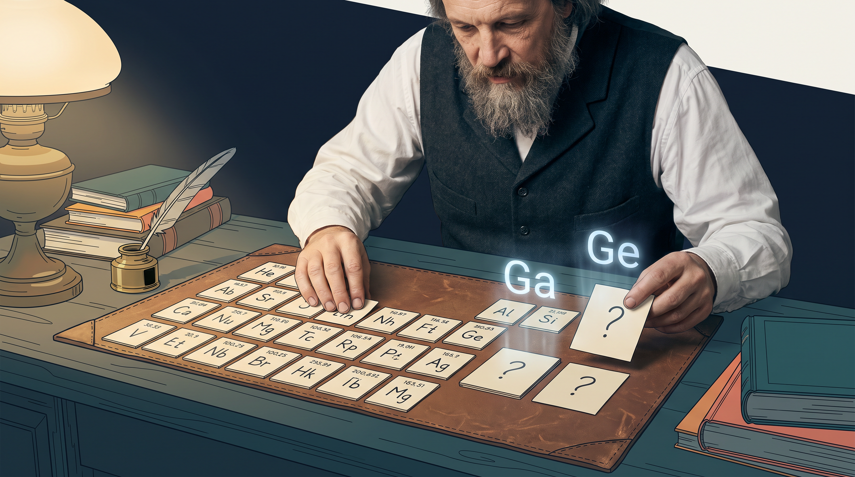
Fig. 3.0 – Mendeleev and the prediction of eka-aluminium and eka-silicon.
This chapter will give you the reasoning tools to answer each of these questions for yourself.
3.1 Why Do We Need to Classify Elements?
Everything around you — the air you breathe, the water you drink, the metal casing of your phone — is built from a small set of basic substances called elements. An element cannot be broken down into anything simpler by ordinary chemical means. This is why we treat elements as the basic units of all types of matter.
The number of known elements has grown steadily over time. In 1800, only 31 elements were known. By 1865, that number had more than doubled to 63, and at present 114 elements are known. Some of the most recently discovered ones do not occur in nature at all; they are man-made, created in the laboratory, and efforts to synthesise still newer elements are continuing. The steady rise in the number of known elements is easy to picture as a simple timeline, shown in Fig. 3.1.
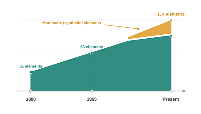
Fig. 3.1 – Growth in the number of known elements over time.
Why We Group Elements
With such a large number of elements, it becomes very difficult to study the chemistry of each one individually, together with their innumerable compounds. Imagine trying to learn the behaviour of every single element in isolation — the task would be almost endless, and we would never see the connections between them.
To ease this problem, scientists searched for a systematic way to organise their knowledge by classifying the elements. A good classification does two powerful things. First, it rationalizes the chemical facts we already know, by placing elements that behave alike into the same groups. Second — and this is the truly remarkable part — it can even help us predict the properties of elements that have not yet been discovered or studied, pointing chemists toward fresh directions for further research.
In the sections that follow, we will trace the historical development of the Periodic Table as it stands today, arrive at the Modern Periodic Law, see how the periodic classification follows as a logical consequence of the electronic configuration of atoms, and finally examine the periodic trends in the physical and chemical properties of the elements.
3.2 Genesis of Periodic Classification
The Periodic Law and the Periodic Table did not appear overnight. They grew slowly, as the consequence of many scientists patiently systematising the knowledge gained through their observations and experiments. Each researcher noticed a small piece of the pattern, and the next built upon it. Before we look at the final table, it is worth walking through these early attempts, because each one teaches us something about how a good classification is judged.
A recurring idea in this story is that certain properties of elements seem to repeat at regular intervals when the elements are lined up by their atomic weight. Here, atomic weight simply means the relative mass of an atom of the element compared with a standard. As we shall see, spotting where the repetition happens is exactly what allowed chemists to organise the elements.
Döbereiner’s Triads
The German chemist Johann Döbereiner, in the early 1800s, was the first to seriously consider the idea of trends among the properties of elements. By 1829, he had noticed a similarity among the physical and chemical properties of several groups of three elements, which he called Triads.
In each triad, he observed something remarkable about the middle element. Its atomic weight fell about half way between the atomic weights of the other two, and its properties, too, lay in between those of the other two members. The triads he identified are listed in Table 3.1.
Table 3.1 Döbereiner’s Triads
| Element | Atomic weight | Element | Atomic weight | Element | Atomic weight |
|---|---|---|---|---|---|
| Li | 7 | Ca | 40 | Cl | 35.5 |
| Na | 23 | Sr | 88 | Br | 80 |
| K | 39 | Ba | 137 | I | 127 |
Notice, for example, that sodium’s atomic weight of 23 is very close to the average of lithium (7) and potassium (39), which is \(\frac{7+39}{2}=23\). This numerical regularity, referred to as the Law of Triads, was the first hint that the properties of elements might be linked to their atomic weights in a systematic way.
However, the relationship seemed to work only for a few sets of elements. Because it could not be extended to most of the known elements, it was dismissed at the time as a mere coincidence.
de Chancourtois and Newlands
The next reported attempt to classify the elements was made by the French geologist A. E. B. de Chancourtois in 1862. He arranged the then-known elements in order of increasing atomic weight and wrapped them around a cylinder, making a cylindrical table designed to display the periodic recurrence of properties. This clever idea, unfortunately, did not attract much attention.
A few years later, in 1865, the English chemist John Alexander Newlands put forward the Law of Octaves. He arranged the elements in increasing order of their atomic weights and noticed that every eighth element had properties similar to the first, as shown in Table 3.2.
The comparison he drew was musical. In the octaves of music, the eighth note resembles the first, and Newlands saw the same kind of repeat-after-eight pattern in the elements.
Table 3.2 Newlands’ Octaves
| Element | Li | Be | B | C | N | O | F |
|---|---|---|---|---|---|---|---|
| At. wt. | 7 | 9 | 11 | 12 | 14 | 16 | 19 |
| Element | Na | Mg | Al | Si | P | S | Cl |
| At. wt. | 23 | 24 | 27 | 29 | 31 | 32 | 35.5 |
| Element | K | Ca | |||||
| At. wt. | 39 | 40 |
Newlands’ Law of Octaves seemed to hold true only for the elements up to calcium; beyond that, the pattern broke down. Although his idea was not widely accepted in his own time, his contribution was recognised much later, when he was awarded the Davy Medal in 1887 by the Royal Society, London.
Meyer and Mendeleev
The Periodic Law, as we understand it today, owes its development chiefly to two chemists working independently: the Russian chemist Dmitri Mendeleev (1834–1907) and the German chemist Lothar Meyer (1830–1895).
In 1869, both proposed that when elements are arranged in the increasing order of their atomic weights, similarities in their physical and chemical properties appear at regular intervals.
Lothar Meyer approached this graphically. He plotted physical properties such as atomic volume, melting point, and boiling point against atomic weight, and obtained a curve that rose and fell in a repeating, periodically recurring pattern. Unlike Newlands, who assumed a fixed repeat of eight, Meyer observed that the length of the repeating pattern actually changed as one moved through the elements — an important and more realistic insight.
By 1868, Meyer had developed a table of elements that closely resembles the Modern Periodic Table. However, his work was not published until after that of Mendeleev, who is therefore generally credited with the development of the Modern Periodic Table.
Mendeleev’s Periodic Law
While Döbereiner had initiated the study of periodic relationships, it was Mendeleev who was responsible for publishing the Periodic Law for the first time.
Mendeleev arranged the elements in horizontal rows and vertical columns of a table, in order of their increasing atomic weights, in such a way that elements with similar properties fell into the same vertical column, or group.
His system was more elaborate than Meyer’s. Mendeleev fully recognised the significance of periodicity and used a broader range of physical and chemical properties to classify the elements. In particular, he relied heavily on the similarities in the empirical formulas and properties of the compounds that the elements formed. In other words, he did not judge an element by the element alone, but also by the kinds of oxides, hydrides, and chlorides it produced.
Gaps and Predictions
Mendeleev soon realised that some elements simply did not fit his scheme if the order of atomic weight was followed too strictly. His response was daring. He decided that the atomic weight measurements of the day might be slightly incorrect, and he chose to place elements with similar properties together even when this meant breaking the strict weight order.
For example, iodine has a lower atomic weight than tellurium, yet Mendeleev placed iodine after tellurium so that it would sit with the other similar elements — fluorine, chlorine, and bromine — in the same family, as reflected in his table (Fig. 3.2). He trusted chemical behaviour over a raw number.
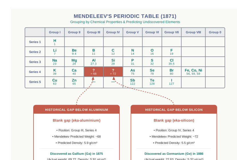
Fig. 3.2 – Mendeleev’s original Periodic Table.
Keeping his primary aim of grouping similar elements together, Mendeleev did something even bolder. He proposed that some elements were still undiscovered, and he deliberately left several gaps in his table for them. At the time, both gallium and germanium were unknown. He left a gap under aluminium and another under silicon, and named these missing elements Eka-Aluminium and Eka-Silicon.
Mendeleev did not merely predict that these elements existed; he described some of their general physical properties in advance. When gallium and germanium were later discovered, the properties measured for them matched Mendeleev’s predictions with striking accuracy, as shown in Table 3.3.
Table 3.3 Mendeleev’s Predictions for the Elements Eka-aluminium (Gallium) and Eka-silicon (Germanium)
| Property | Eka-aluminium (predicted) | Gallium (found) | Eka-silicon (predicted) | Germanium (found) |
|---|---|---|---|---|
| Atomic weight | 68 | 70 | 72 | 72.6 |
| Density / (g/cm³) | 5.9 | 5.94 | 5.5 | 5.36 |
| Melting point / K | Low | 302.93 | High | 1231 |
| Formula of oxide | \(\mathrm{E_2O_3}\) | \(\mathrm{Ga_2O_3}\) | \(\mathrm{EO_2}\) | \(\mathrm{GeO_2}\) |
| Formula of chloride | \(\mathrm{ECl_3}\) | \(\mathrm{GaCl_3}\) | \(\mathrm{ECl_4}\) | \(\mathrm{GeCl_4}\) |
The boldness of these quantitative predictions, and their eventual success, is what made Mendeleev and his Periodic Table famous. A version of Mendeleev’s Periodic Table, as published in 1905, is shown in Fig. 3.2.
Taken together, these attempts show a clear line of progress, which is easiest to appreciate side by side.
3.3 Modern Periodic Law and the Present Form of the Periodic Table
We must keep one important fact in mind: when Mendeleev built his Periodic Table, chemists knew nothing about the internal structure of the atom. They had no idea about protons, electrons, or the arrangement of electrons. Mendeleev’s ordering by atomic weight was, in a sense, the best that could be done at the time.
The beginning of the twentieth century, however, witnessed profound developments in the theories about sub-atomic particles. Once the atom’s inner structure came to light, the true basis of the Periodic Table could finally be uncovered.
Moseley and the Atomic Number
In 1913, the English physicist Henry Moseley studied the characteristic X-rays given off by different elements. Every element, when bombarded suitably, emits X-rays of a frequency that is characteristic of that element — a kind of fingerprint.
Moseley looked for a regular relationship between this X-ray frequency and the identity of the element. He found that a plot of \(\sqrt{\nu}\) (where \(\nu\) is the frequency of the X-rays emitted) against the atomic number \(Z\) gave a straight line. Crucially, plotting \(\sqrt{\nu}\) against atomic mass did not give such a clean straight line.
This was a decisive result. A property that varies in a simple, straight-line fashion with atomic number, but not with atomic mass, is telling us that the atomic number — not the atomic mass — is the more fundamental property of an element. The atomic number, you may recall, is equal to the nuclear charge, that is, the number of protons in the nucleus, and in a neutral atom it also equals the number of electrons.
Because of Moseley’s work, Mendeleev’s Periodic Law was accordingly modified. Atomic weight was replaced by atomic number as the ordering principle, giving us what we now call the Modern Periodic Law.
Why Electronic Configuration is the Real Basis
Once we accept that atomic number governs periodicity, its deeper meaning becomes clear. Since the atomic number fixes the number of electrons in a neutral atom, it also fixes how those electrons are arranged — the electronic configuration.
It is now recognised that the Periodic Law is essentially the consequence of the periodic variation in electronic configurations. As we move through the elements, the pattern of filling electrons into shells and orbitals repeats itself, and it is this repeating pattern of configurations that indeed determines the physical and chemical properties of elements and their compounds.
The Modern Periodic Law revealed important analogies among the 94 naturally occurring elements. Even elements once thought purely artificial, such as neptunium and plutonium, are, like actinium and protoactinium, found in trace amounts in pitchblende — an ore of uranium. This law renewed interest in Inorganic Chemistry and has carried into the present day, extended further by the creation of artificially produced short-lived elements.
The Long Form of the Periodic Table
Numerous forms of the Periodic Table have been devised from time to time. Some forms emphasise chemical reactions and valence, while others stress the electronic configuration of elements. The modern version most widely used is the so-called “long form” of the Periodic Table, shown in Fig. 3.3. It is the most convenient and is the one we shall use throughout.
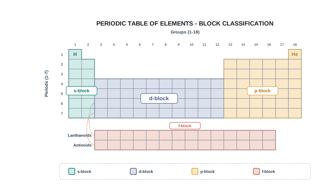
Fig. 3.3 – The long form of the modern Periodic Table.
In this table, the horizontal rows — which Mendeleev had called series — are now called periods, and the vertical columns are called groups. Elements having similar outer electronic configurations in their atoms are placed one below another in the same vertical column, which is why groups are also called families.
Following the recommendation of the International Union of Pure and Applied Chemistry (IUPAC), the groups are numbered from 1 to 18. This simple numbering replaces the older, more confusing notation of groups IA to VIIA, VIII, IB to VIIB, and 0.
Periods and Groups
There are altogether seven periods. The period number corresponds to the highest principal quantum number (\(n\)) of the elements in that period. Here, the principal quantum number \(n\) is the number that labels the main energy level, or shell, of an electron.
The first period contains only 2 elements. The subsequent periods consist of 8, 8, 18, 18, and 32 elements, respectively. The seventh period is still incomplete; like the sixth period, it would have a theoretical maximum of 32 elements based on the number of available quantum numbers.
In this form of the Periodic Table, 14 elements each of the sixth and seventh periods — the lanthanoids and the actinoids, respectively — are placed in separate panels at the bottom. This is done purely to keep the main table compact and readable; otherwise the table would become inconveniently wide.
3.4 Nomenclature of Elements with Atomic Numbers > 100
Why Naming Became a Problem
Traditionally, the naming of a newly discovered element was the privilege of its discoverer (or discoverers), and the suggested name was then ratified by IUPAC. In recent years, however, this simple tradition has led to some controversy.
The reason lies in the nature of the newest elements. Those with very high atomic numbers are so unstable — that is, so quickly radioactive — that only minute quantities, sometimes only a few atoms, can ever be obtained. Their synthesis and characterisation (confirming exactly which element has been made and measuring its properties) therefore require highly sophisticated and costly equipment and laboratories.
Such work is carried out with a competitive spirit in only a handful of laboratories around the world. Under this pressure, scientists have sometimes been tempted to claim a discovery even before collecting reliable data on the new element.
A famous case is element 104. Both American and Soviet scientists claimed the credit for discovering it. The Americans named it Rutherfordium, whereas the Soviets named it Kurchatovium — leaving the world with two names for one element.
The IUPAC Systematic Names
To avoid such problems, IUPAC recommended that until a new element’s discovery is proved and its name is officially recognised, a systematic name should be derived directly from the atomic number of the element. This is done using fixed numerical roots for 0 and for the numbers 1 to 9, listed in Table 3.4.
Table 3.4 Notation for IUPAC Nomenclature of Elements
| Digit | Name | Abbreviation |
|---|---|---|
| 0 | nil | n |
| 1 | un | u |
| 2 | bi | b |
| 3 | tri | t |
| 4 | quad | q |
| 5 | pent | p |
| 6 | hex | h |
| 7 | sept | s |
| 8 | oct | o |
| 9 | enn | e |
The rule is simple: take the digits that make up the atomic number, replace each digit by its root, join the roots together in the same order as the digits, and add “ium” at the end. The three-letter symbol is formed by joining the abbreviations of the same roots. The full sequence of steps is summarised in FC 3.1.
Flowchart
FC 3.1 – IUPAC systematic naming: atomic number → split into individual digits → replace each digit with its numerical root (Table 3.4) → join the roots in order → add “ium” to get the temporary name; in parallel, join the digit abbreviations to get the three-letter symbol → later, IUPAC vote assigns the permanent name and symbol.
The systematic IUPAC names for the elements with \(Z\) above 100 are shown in Table 3.5, alongside the permanent official names that IUPAC has since assigned.
Table 3.5 Nomenclature of Elements with Atomic Number Above 100
| Atomic Number | Name according to IUPAC nomenclature | Symbol | IUPAC Official Name | IUPAC Symbol |
|---|---|---|---|---|
| 101 | Unnilunium | Unu | Mendelevium | Md |
| 102 | Unnilbium | Unb | Nobelium | No |
| 103 | Unniltrium | Unt | Lawrencium | Lr |
| 104 | Unnilquadium | Unq | Rutherfordium | Rf |
| 105 | Unnilpentium | Unp | Dubnium | Db |
| 106 | Unnilhexium | Unh | Seaborgium | Sg |
| 107 | Unnilseptium | Uns | Bohrium | Bh |
| 108 | Unniloctium | Uno | Hassium | Hs |
| 109 | Unnilennium | Une | Meitnerium | Mt |
| 110 | Ununnillium | Uun | Darmstadtium | Ds |
| 111 | Unununnium | Uuu | Rontgenium | Rg |
| 112 | Ununbium | Uub | Copernicium | Cn |
| 113 | Ununtrium | Uut | Nihonium | Nh |
| 114 | Ununquadium | Uuq | Flerovium | Fl |
| 115 | Ununpentium | Uup | Moscovium | Mc |
| 116 | Ununhexium | Uuh | Livermorium | Lv |
| 117 | Ununseptium | Uus | Tennessine | Ts |
| 118 | Ununoctium | Uuo | Oganesson | Og |
From Temporary to Permanent Names
In this way, a newly made element first receives a temporary name, with a symbol consisting of three letters. Later, once its discovery is firmly established, a permanent name and symbol are decided by a vote of IUPAC representatives from each country.
The permanent name might reflect the country (or the state within a country) in which the element was discovered, or it may pay tribute to a notable scientist. You can see both kinds of tribute in Table 3.5 — for instance, Nihonium (after Japan) and Mendelevium (after Mendeleev).
As of now, elements with atomic numbers up to 118 have been discovered, and the official names of all these elements have been announced by IUPAC.
3.5 Electronic Configurations of Elements and the Periodic Table
In the preceding chapter you learnt that an electron in an atom is described by a set of four quantum numbers, and that the principal quantum number (\(n\)) defines the main energy level, known as a shell. You also studied how electrons are filled into different subshells, also called orbitals (\(s\), \(p\), \(d\), \(f\)), within an atom.
The distribution of electrons into the orbitals of an atom is called its electronic configuration. As a quick reminder, the four subshell types can hold different numbers of electrons: an \(s\) subshell holds up to 2, a \(p\) subshell up to 6, a \(d\) subshell up to 10, and an \(f\) subshell up to 14 electrons. These numbers will matter throughout this section.
An element’s location in the Periodic Table reflects the quantum numbers of the last orbital that was filled. In this section we will see the direct and beautiful connection between the electronic configurations of the elements and the long form of the Periodic Table.
Electronic Configurations Across Periods
The period tells us the value of \(n\) for the outermost, or valence, shell. In other words, each successive period in the Periodic Table is associated with the filling of the next higher principal energy level (\(n = 1\), then \(n = 2\), and so on).
A very useful rule follows from this: the number of elements in any period is exactly twice the number of atomic orbitals available in the energy level being filled. (The factor of two appears because each orbital holds two electrons, and each electron added means one more element.)
The First Three Periods
The first period (\(n = 1\)) begins with the filling of the lowest available level, \(1s\). Since there is only one \(1s\) orbital, it holds two electrons, so this period has just two elements — hydrogen (\(1s^1\)) and helium (\(1s^2\)) — after which the first shell (the K shell) is complete.
The second period (\(n = 2\)) starts with lithium, whose third electron enters the \(2s\) orbital. Beryllium, with four electrons, has the configuration \(1s^2\,2s^2\). From the next element, boron, the \(2p\) orbitals begin to fill, and the L shell is completed at neon (\(2s^2\,2p^6\)). Thus the second period contains 8 elements.
The third period (\(n = 3\)) begins at sodium, where the added electron enters a \(3s\) orbital. The successive filling of the \(3s\) and \(3p\) orbitals then gives a third period of 8 elements, from sodium to argon.
Where the Transition Series Appear
The fourth period (\(n = 4\)) starts at potassium, and the added electrons first fill the \(4s\) orbital. Now something new happens. Before the \(4p\) orbital fills, the filling of the \(3d\) orbitals becomes energetically more favourable, and we meet the so-called \(3d\) transition series of elements.
This filling order — where \(4s\) fills before \(3d\) — is not a mistake; it happens because, at this stage, the \(4s\) orbital is actually slightly lower in energy than the \(3d\). The \(3d\) transition series starts from scandium (\(Z = 21\)), which has the configuration \(3d^1\,4s^2\), and the \(3d\) orbitals are completely filled at zinc (\(Z = 30\)), with configuration \(3d^{10}\,4s^2\). The fourth period then ends at krypton with the filling of the \(4p\) orbitals. Altogether there are 18 elements in this fourth period.
The fifth period (\(n = 5\)), beginning with rubidium, is similar to the fourth period and contains the \(4d\) transition series, which starts at yttrium (\(Z = 39\)). This period ends at xenon with the filling of the \(5p\) orbitals.
The Inner Transition Series
The sixth period (\(n = 6\)) contains 32 elements. Here, successive electrons enter the \(6s\), \(4f\), \(5d\), and \(6p\) orbitals, in that broad order. The filling of the \(4f\) orbitals begins with cerium (\(Z = 58\)) and ends at lutetium (\(Z = 71\)), giving the \(4f\)-inner transition series, which is called the lanthanoid series.
The seventh period (\(n = 7\)) is similar to the sixth, with the successive filling of the \(7s\), \(5f\), \(6d\), and \(7p\) orbitals, and it includes most of the man-made radioactive elements. This period will end at the element with atomic number 118, which would belong to the noble gas family. The filling of the \(5f\) orbitals, beginning after actinium (\(Z = 89\)), gives the \(5f\)-inner transition series, known as the actinoid series.
The overall order in which orbitals are filled as we build up the elements is worth having at a glance, and is shown in FC 3.2.
Flowchart
FC 3.2 – Order of orbital filling (aufbau order): 1s → 2s → 2p → 3s → 3p → 4s → 3d → 4p → 5s → 4d → 5p → 6s → 4f → 5d → 6p → 7s → 5f → 6d → 7p; mark 3d/4d/5d/6d as the transition-series entries and 4f/5f as the inner-transition (lanthanoid/actinoid) entries.
The \(4f\)- and \(5f\)-inner transition series are placed separately at the bottom of the Periodic Table. This is done to keep the table’s structure neat and, more importantly, to preserve the principle of classification by keeping elements with similar properties in a single column.
Group-wise Electronic Configurations
Elements in the same vertical column, or group, have similar valence shell electronic configurations. They possess the same number of electrons in their outer orbitals, and this is precisely why they show similar chemical properties.
For example, the Group 1 elements (the alkali metals) all have an \(ns^1\) valence shell electronic configuration, as shown below.
| Atomic number | Symbol | Electronic configuration |
|---|---|---|
| 3 | Li | \(1s^2\,2s^1\) (or) \([\mathrm{He}]\,2s^1\) |
| 11 | Na | \(1s^2\,2s^2\,2p^6\,3s^1\) (or) \([\mathrm{Ne}]\,3s^1\) |
| 19 | K | \(1s^2\,2s^2\,2p^6\,3s^2\,3p^6\,4s^1\) (or) \([\mathrm{Ar}]\,4s^1\) |
| 37 | Rb | \(1s^2\,2s^2\,2p^6\,3s^2\,3p^6\,3d^{10}\,4s^2\,4p^6\,5s^1\) (or) \([\mathrm{Kr}]\,5s^1\) |
| 55 | Cs | \(1s^2\,2s^2\,2p^6\,3s^2\,3p^6\,3d^{10}\,4s^2\,4p^6\,4d^{10}\,5s^2\,5p^6\,6s^1\) (or) \([\mathrm{Xe}]\,6s^1\) |
| 87 | Fr | \([\mathrm{Rn}]\,7s^1\) |
Notice that although lithium and caesium differ enormously in atomic mass, they share the same \(ns^1\) outer configuration — and that shared outer arrangement is what makes them all soft, reactive alkali metals.
Thus we can clearly see that the properties of an element have a periodic dependence upon its atomic number, and not upon its relative atomic mass.
3.6 Electronic Configurations and Types of Elements: s-, p-, d-, f- Blocks
The aufbau (build-up) principle, together with the electronic configuration of atoms, provides a solid theoretical foundation for the periodic classification. Recall that the aufbau principle simply says electrons fill the lowest-energy orbitals first as we build up an atom.
The elements in a vertical column of the Periodic Table make up a group, or family, and show similar chemical behaviour. This similarity arises because these elements have the same number, and the same distribution, of electrons in their outermost orbitals.
We can classify all the elements into four blocks — the s-block, p-block, d-block, and f-block — depending on the type of atomic orbital that is being filled with electrons. This block structure is illustrated in Fig. 3.4.
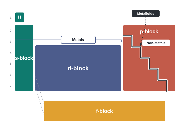
Fig. 3.4 – The s-, p-, d-, and f-blocks of the Periodic Table.
There are two exceptions worth noting at once. Strictly, helium belongs to the s-block (its configuration is \(1s^2\)), yet it is positioned in the p-block along with the other Group 18 elements. This is justified because its completely filled valence shell (\(1s^2\)) makes it behave exactly like the other noble gases.
The other exception is hydrogen. With only one s-electron, it can be placed in Group 1 with the alkali metals. But it can also gain one electron to reach a noble-gas arrangement, which makes it resemble a Group 17 (halogen) element. Because it is such a special case, hydrogen is placed separately at the top of the Periodic Table, as shown in Fig. 3.3 and Fig. 3.4.
A quick side-by-side view of the four blocks makes their differences easy to hold in mind.
We will now briefly discuss the salient features of these four types of elements. Some of the terms used here — such as ionization enthalpy and electron gain enthalpy — will be defined properly in Section 3.7; for now, ionization enthalpy can be read simply as a measure of how easily an atom loses an electron.
3.6.1 The s-Block Elements
The elements of Group 1 (the alkali metals) and Group 2 (the alkaline earth metals), which have \(ns^1\) and \(ns^2\) outermost electronic configurations respectively, belong to the s-Block Elements.
These are all reactive metals with low ionization enthalpies, meaning they give up their outer electrons easily. They lose the outermost electron(s) readily to form a 1+ ion (in the case of the alkali metals) or a 2+ ion (in the case of the alkaline earth metals).
The metallic character and the reactivity both increase as we go down the group. Because of this high reactivity, s-block elements are never found pure (in the free state) in nature; they always occur combined with other elements. The compounds of the s-block elements are predominantly ionic, with the important exception of those of lithium and beryllium, which show more covalent character.
3.6.2 The p-Block Elements
The p-Block Elements are those belonging to Groups 13 to 18. Together with the s-Block Elements, they are called the Representative Elements or Main Group Elements.
Their outermost electronic configuration varies from \(ns^2np^1\) to \(ns^2np^6\) across each period. At the end of every period sits a noble gas, with a closed valence shell of \(ns^2np^6\).
All the orbitals in the valence shell of the noble gases are completely filled with electrons, and it is very difficult to disturb this stable arrangement by adding or removing electrons. This is why the noble gases show very low chemical reactivity.
Just before the noble gas family lie two chemically important groups of non-metals: the halogens (Group 17) and the chalcogens (Group 16). These two groups have highly negative electron gain enthalpies and readily add one or two electrons, respectively, to attain the stable noble-gas configuration.
Across a period, the non-metallic character increases as we move from left to right, while down a group the metallic character increases.
3.6.3 The d-Block Elements (Transition Elements)
These are the elements of Groups 3 to 12, sitting in the centre of the Periodic Table. They are characterised by the filling of inner \(d\) orbitals by electrons, and are therefore referred to as the d-Block Elements.
Their general outer electronic configuration is \((n-1)d^{1-10}ns^{0-2}\), with the exception of palladium (Pd), whose configuration is \(4d^{10}5s^0\). They are all metals. They mostly form coloured ions, exhibit variable valence (that is, several oxidation states), show paramagnetism (attraction to a magnetic field, arising from unpaired electrons), and are frequently used as catalysts.
However, zinc, cadmium, and mercury, which have the electronic configuration \((n-1)d^{10}ns^2\), do not show most of the properties of transition elements, because their \(d\) subshell is completely filled.
In a way, the transition metals form a bridge between the chemically active metals of the s-block and the less active elements of Groups 13 and 14 — and it is from this “in-between” position that they take their familiar name, “Transition Elements.”
3.6.4 The f-Block Elements (Inner-Transition Elements)
The two rows of elements placed at the bottom of the Periodic Table are the Lanthanoids, from cerium, Ce (\(Z = 58\)), to lutetium, Lu (\(Z = 71\)), and the Actinoids, from thorium, Th (\(Z = 90\)), to lawrencium, Lr (\(Z = 103\)).
They are characterised by the outer electronic configuration \((n-2)f^{1-14}(n-1)d^{0-1}ns^2\). Because the last electron added to each of these elements enters an \(f\)-orbital, these two series are called the Inner-Transition Elements or f-Block Elements.
They are all metals. Within each series, the properties of the elements are quite similar to one another. The chemistry of the early actinoids is more complicated than that of the corresponding lanthanoids, owing to the large number of oxidation states possible for these actinoid elements.
The actinoid elements are radioactive. Many of them have been made only in nanogram quantities, or even less, through nuclear reactions, and their chemistry is therefore not yet fully studied. The elements that come after uranium are called the Transuranium Elements.
3.6.5 Metals, Non-metals and Metalloids
In addition to the classification into s-, p-, d-, and f-blocks, Fig. 3.4 shows another broad classification of elements based on their properties: they can be divided into Metals and Non-Metals.
Metals comprise more than 78% of all known elements and appear on the left side of the Periodic Table. Metals are usually solids at room temperature — mercury is an exception (it is a liquid), while gallium and caesium also have very low melting points (\(303\ \text{K}\) and \(302\ \text{K}\), respectively). Metals usually have high melting and boiling points, are good conductors of heat and electricity, and are both malleable (can be flattened into thin sheets by hammering) and ductile (can be drawn into wires).
Non-metals, in contrast, are located at the top right-hand side of the Periodic Table. In fact, along any horizontal row, the character of the elements changes from metallic on the left to non-metallic on the right. Non-metals are usually solids or gases at room temperature, with low melting and boiling points (boron and carbon are exceptions). They are poor conductors of heat and electricity, and most non-metallic solids are brittle — neither malleable nor ductile.
The elements become more metallic as we go down a group, whereas the non-metallic character increases as we move from left to right across the Periodic Table.
This change from metallic to non-metallic character is not abrupt. It is marked by the thick zig-zag line shown in Fig. 3.4. The elements that border this line and run diagonally across the table — such as silicon, germanium, arsenic, antimony, and tellurium — show properties characteristic of both metals and non-metals. These elements are called Semi-metals or Metalloids.
3.7 Periodic Trends in Properties of Elements
There are many observable patterns in the physical and chemical properties of elements as we descend a group or move across a period in the Periodic Table.
For example, within a period, chemical reactivity tends to be high in the Group 1 metals, lower in the elements towards the middle of the table, and then increases again to a maximum in the Group 17 non-metals. Likewise, within a group of representative metals (say the alkali metals), reactivity increases on moving down the group, whereas within a group of non-metals (say the halogens), reactivity decreases down the group.
But why do the properties of elements follow these trends? And how can we explain periodicity at all? To answer these questions, we must look into the atomic structure and the way electrons are arranged. In this section we shall discuss the periodic trends in certain physical and chemical properties and try to explain them in terms of the number of electrons and their energy levels.
3.7.1 Trends in Physical Properties
There are numerous physical properties of elements — such as melting and boiling points, heats of fusion and vaporization, and energy of atomization — that show periodic variations. Here, however, we shall focus on the periodic trends in atomic and ionic radii, ionization enthalpy, electron gain enthalpy, and electronegativity.
Atomic Radius
You can well imagine that finding the size of an atom is much more complicated than measuring the radius of a ball. Do you know why? Firstly, the size of an atom (with a radius of about \(1.2\ \text{Å}\), that is, \(1.2\times10^{-10}\ \text{m}\)) is extremely small. Secondly, the electron cloud surrounding the atom does not have a sharp boundary, so its size cannot be pinned down precisely. In other words, there is no practical way to measure the size of an individual, isolated atom directly.
However, we can estimate atomic size indirectly, by measuring the distance between atoms in the combined state — that is, in molecules and crystals.
For a non-metallic element, one practical approach is to measure the distance between two atoms joined by a single bond in a covalent molecule, and take half of that distance as the atom’s radius.
For example, the bond distance in the chlorine molecule (\(\mathrm{Cl_2}\)) is 198 pm, and half of this distance, 99 pm, is taken as the atomic (covalent) radius of chlorine.
For metals, we use a similar idea in the metallic crystal.
For example, the distance between two adjacent copper atoms in solid copper is 256 pm, so the metallic radius of copper is assigned a value of 128 pm.
For simplicity, in this book we use the single term atomic radius to refer to either the covalent radius or the metallic radius, depending on whether the element is a non-metal or a metal. Atomic radii can be measured by X-ray or other spectroscopic methods.
The atomic radii of a few elements are listed in Table 3.6(a), from which two clear trends emerge. We can explain both in terms of nuclear charge and energy level.
Table 3.6(a) Atomic Radii / pm Across the Periods
| Atom (Period II) | Li | Be | B | C | N | O | F |
|---|---|---|---|---|---|---|---|
| Atomic radius | 152 | 111 | 88 | 77 | 74 | 66 | 64 |
| Atom (Period III) | Na | Mg | Al | Si | P | S | Cl |
| Atomic radius | 186 | 160 | 143 | 117 | 110 | 104 | 99 |
The first trend is that atomic size generally decreases across a period, as illustrated in Fig. 3.5(a) for the elements of the second period. This happens because, within a period, the outer electrons are all being added to the same valence shell, while the effective nuclear charge — the net positive pull actually felt by an outer electron — increases as the atomic number increases. The rising pull draws the electrons closer to the nucleus, so the atom shrinks.
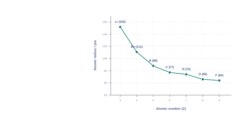
Fig. 3.5(a) – Variation of atomic radius across the second period.
The second trend is that within a family, or vertical column, the atomic radius increases regularly with atomic number, as illustrated in Fig. 3.5(b) for the alkali metals and the halogens. As we descend a group, the principal quantum number (\(n\)) increases, so the valence electrons occupy shells that are farther from the nucleus. Moreover, the inner shells, now filled with electrons, shield the outer electrons from the pull of the nucleus. Consequently, the size of the atom increases down the group.
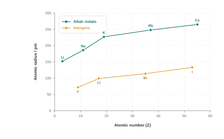
Fig. 3.5(b) – Variation of atomic radius down a group.
Table 3.6(b) Atomic Radii / pm Down a Family
| Atom (Group I) | Atomic Radius | Atom (Group 17) | Atomic Radius |
|---|---|---|---|
| Li | 152 | F | 64 |
| Na | 186 | Cl | 99 |
| K | 231 | Br | 114 |
| Rb | 244 | I | 133 |
| Cs | 262 | At | 140 |
Note that the atomic radii of the noble gases are not considered here. Being monoatomic, their non-bonded radii are very large. In fact, the radii of noble gases should be compared not with the covalent radii but with the van der Waals radii of the other elements.
Ionic Radius
The removal of an electron from an atom results in the formation of a cation (a positive ion), whereas the gain of an electron leads to an anion (a negative ion). The ionic radii can be estimated by measuring the distances between cations and anions in ionic crystals.
In general, the ionic radii of elements exhibit the same trends as the atomic radii. A cation is always smaller than its parent atom, because it has fewer electrons while its nuclear charge remains the same — the same nucleus now pulls in a smaller electron cloud.
For example, the atomic radius of sodium is 186 pm, compared with an ionic radius of only 95 pm for \(\mathrm{Na^+}\).
The size of an anion, on the other hand, is always larger than that of its parent atom, because adding one or more electrons increases the repulsion among the electrons and decreases the effective nuclear charge per electron. For example, the ionic radius of the fluoride ion (\(\mathrm{F^-}\)) is 136 pm, whereas the atomic radius of fluorine is only 64 pm.
When some atoms and ions contain the same number of electrons, we call them isoelectronic species.
For example, \(\mathrm{O^{2-}}\), \(\mathrm{F^-}\), \(\mathrm{Na^+}\), and \(\mathrm{Mg^{2+}}\) all have the same number of electrons (10). Their radii differ, however, because of their different nuclear charges. Among such isoelectronic species, the one with the greater positive nuclear charge will have the smaller radius, because the greater positive charge pulls the fixed set of electrons in more tightly. Conversely, an anion with a greater negative charge has the larger radius, because the net repulsion among the electrons outweighs the nuclear charge and the ion expands in size.
Ionization Enthalpy
A quantitative measure of the tendency of an element to lose an electron is given by its ionization enthalpy. It represents the energy required to remove an electron from an isolated gaseous atom (X) in its ground state.
\[\mathrm{X}\text{(g)} \rightarrow \mathrm{X^+}\text{(g)} + \mathrm{e^-} \qquad (3.1)\]
The ionization enthalpy is expressed in units of \(\text{kJ mol}^{-1}\). We can similarly define the second ionization enthalpy as the energy required to remove the second most loosely bound electron, that is, the energy for the reaction in equation 3.2.
\[\mathrm{X^+}\text{(g)} \rightarrow \mathrm{X^{2+}}\text{(g)} + \mathrm{e^-} \qquad (3.2)\]
Because energy is always required to pull an electron away from an atom, ionization enthalpies are always positive. The second ionization enthalpy is higher than the first, because it is more difficult to remove an electron from a positively charged ion than from a neutral atom. In the same way, the third ionization enthalpy is higher than the second, and so on. When we say “ionization enthalpy” without qualification, we mean the first ionization enthalpy.
The first ionization enthalpies of elements with atomic numbers up to 60 are plotted in Fig. 3.6, and the periodicity of the graph is striking.
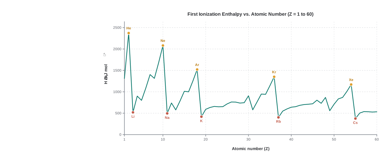
Fig. 3.6 – Variation of first ionization enthalpy with atomic number.
You will find maxima at the noble gases, which have closed electron shells and very stable electronic configurations. On the other hand, minima occur at the alkali metals, whose low ionization enthalpies match their high reactivity.
In addition, two general trends stand out: the first ionization enthalpy generally increases across a period and decreases down a group. These trends are illustrated in Figs. 3.7(a) and 3.7(b), for the second period and the first group respectively.
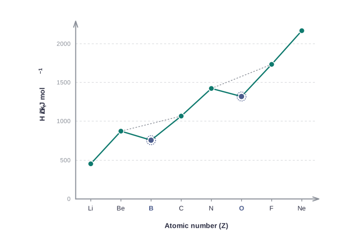
Fig. 3.7(a) – First ionization enthalpy across the second period.
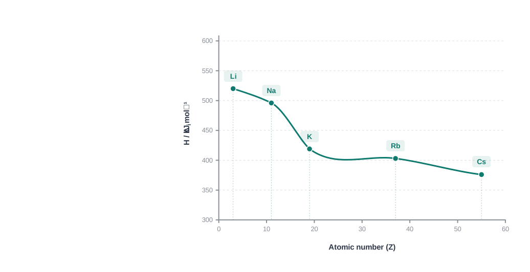
Fig. 3.7(b) – First ionization enthalpy down the alkali metal group.
You will appreciate that ionization enthalpy and atomic radius are closely related. To understand these trends, we must consider two factors: (i) the attraction of the electrons towards the nucleus, and (ii) the repulsion of the electrons from one another.
The effective nuclear charge experienced by a valence electron is less than the actual charge on the nucleus, because of the “shielding” or “screening” of the valence electron from the nucleus by the intervening core electrons. For example, the \(2s\) electron in lithium is shielded from the nucleus by the inner core of \(1s\) electrons, so the valence electron experiences a net positive charge that is less than the full charge of +3. In general, shielding is most effective when the inner orbitals are completely filled — exactly the situation for the alkali metals, with their single outermost \(ns\)-electron preceding a noble-gas core.
When we move from lithium to fluorine across the second period, successive electrons are added to orbitals of the same principal quantum level. The shielding by the inner core does not increase very much, so it cannot compensate for the increased attraction of the electron to the nucleus. Thus, across a period, the increasing nuclear charge outweighs the shielding, the outermost electrons are held more and more tightly, and the ionization enthalpy increases.
As we go down a group, the outermost electron lies increasingly farther from the nucleus, and there is increased shielding of the nuclear charge by the electrons in the inner levels. In this case the increase in shielding outweighs the increasing nuclear charge, so the removal of the outermost electron requires less energy, and ionization enthalpy decreases down a group.
Two Instructive Anomalies
From Fig. 3.7(a), you will notice that the first ionization enthalpy of boron (\(Z = 5\)) is slightly less than that of beryllium (\(Z = 4\)), even though boron has a greater nuclear charge.
The reason lies in the type of electron removed. Within the same principal quantum level, an \(s\)-electron is attracted to the nucleus more strongly than a \(p\)-electron. In beryllium, the electron removed during ionization is a \(2s\)-electron, whereas in boron it is a \(2p\)-electron. Because a \(2s\)-electron penetrates closer to the nucleus than a \(2p\)-electron, the \(2p\)-electron of boron is more shielded by the inner core. It is therefore easier to remove the \(2p\)-electron from boron than the \(2s\)-electron from beryllium, and so boron has the smaller first ionization enthalpy.
A second “anomaly” is the smaller first ionization enthalpy of oxygen compared with nitrogen. This arises from electron pairing. In the nitrogen atom, the three \(2p\)-electrons occupy three different orbitals singly (following Hund’s rule). In the oxygen atom, two of the four \(2p\)-electrons must share the same \(2p\)-orbital, producing extra electron–electron repulsion. Because of this repulsion, it is easier to remove the fourth \(2p\)-electron from oxygen than to remove one of the three from nitrogen.
Electron Gain Enthalpy
When an electron is added to a neutral gaseous atom (X) to convert it into a negative ion, the enthalpy change accompanying the process is defined as the electron gain enthalpy (\(\Delta_{eg}H\)). It provides a measure of the ease with which an atom adds an electron to form an anion, as shown in equation 3.3.
\[\mathrm{X}\text{(g)} + \mathrm{e^-} \rightarrow \mathrm{X^-}\text{(g)} \qquad (3.3)\]
Depending on the element, this process can be either endothermic or exothermic. For many elements, energy is released when an electron is added to the atom, and the electron gain enthalpy is negative. For example, the Group 17 elements (the halogens) have very high (large) negative electron gain enthalpies, because by picking up an electron they attain a stable noble-gas configuration.
On the other hand, the noble gases have large positive electron gain enthalpies, because the incoming electron would have to enter the next higher principal quantum level, leading to a very unstable electronic configuration. It may be noted that electron gain enthalpies have their large negative values towards the upper right of the periodic table, just before the noble gases.
Table 3.7 Electron Gain Enthalpies / (kJ mol⁻¹) of Some Main Group Elements
| Group 1 | \(\Delta_{eg}H\) | Group 16 | \(\Delta_{eg}H\) | Group 17 | \(\Delta_{eg}H\) | Group 0 | \(\Delta_{eg}H\) |
|---|---|---|---|---|---|---|---|
| H | – 73 | He | + 48 | ||||
| Li | – 60 | O | – 141 | F | – 328 | Ne | + 116 |
| Na | – 53 | S | – 200 | Cl | – 349 | Ar | + 96 |
| K | – 48 | Se | – 195 | Br | – 325 | Kr | + 96 |
| Rb | – 47 | Te | – 190 | I | – 295 | Xe | + 77 |
| Cs | – 46 | Po | – 174 | At | – 270 | Rn | + 68 |
The variation in electron gain enthalpies is less systematic than that in ionization enthalpies. As a general rule, electron gain enthalpy becomes more negative with increasing atomic number across a period. This is because the effective nuclear charge increases from left to right, so it becomes easier to add an electron to a smaller atom, where the added electron would, on average, be closer to the positively charged nucleus.
We should also expect the electron gain enthalpy to become less negative as we go down a group, because the size of the atom increases and the added electron would be farther from the nucleus. This is generally the case, as seen in Table 3.7.
However, the electron gain enthalpy of oxygen or fluorine is less negative than that of the element just below it (sulphur or chlorine, respectively). This is because when an electron is added to the small O or F atom, it enters the compact \(n = 2\) level and suffers significant repulsion from the other electrons already crowded there. For the larger \(n = 3\) level (S or Cl), the added electron occupies a bigger region of space, and the electron–electron repulsion is much less.
The quantity related to electron gain enthalpy is the electron affinity. In many books, the negative of the enthalpy change for the process in equation 3.3 is defined as the electron affinity (\(A_e\)) of the atom. If energy is released when an electron is added, the electron affinity is taken as positive (this is the opposite of the thermodynamic convention). Electron affinity is defined at absolute zero, so at any other temperature (T) the heat capacities of reactants and products must be accounted for, giving: \[\Delta_{eg}H = -A_e - \tfrac{5}{2}RT\]
Electronegativity
A qualitative measure of the ability of an atom, in a chemical compound, to attract shared electrons to itself is called electronegativity.
Unlike ionization enthalpy and electron gain enthalpy, electronegativity is not a measurable quantity. However, a number of numerical scales of electronegativity have been developed, such as the Pauling scale, the Mulliken–Jaffe scale, and the Allred–Rochow scale. The most widely used is the Pauling scale. Linus Pauling, an American scientist, in 1922 arbitrarily assigned a value of 4.0 to fluorine, the element considered to have the greatest ability to attract electrons. Approximate electronegativity values for a few elements are given in Table 3.8(a).
The electronegativity of any given element is not constant; it varies depending on the element to which it is bound. Though it is not a measurable quantity, it does provide a valuable means of predicting the nature of the force that holds a pair of atoms together — a relationship you will explore later.
Electronegativity generally increases across a period from left to right (say from lithium to fluorine) and decreases down a group (say from fluorine to astatine). How can these trends be explained? They can be related directly to atomic radii. The attraction between the outer (valence) electrons and the nucleus increases as the atomic radius decreases across a period, so the electronegativity also increases. On the same account, electronegativity values decrease as the atomic radius increases down a group. The overall trend is therefore similar to that of ionization enthalpy.
Table 3.8(a) Electronegativity Values (on Pauling scale) Across the Periods
| Atom (Period II) | Li | Be | B | C | N | O | F |
|---|---|---|---|---|---|---|---|
| Electronegativity | 1.0 | 1.5 | 2.0 | 2.5 | 3.0 | 3.5 | 4.0 |
| Atom (Period III) | Na | Mg | Al | Si | P | S | Cl |
| Electronegativity | 0.9 | 1.2 | 1.5 | 1.8 | 2.1 | 2.5 | 3.0 |
Table 3.8(b) Electronegativity Values (on Pauling scale) Down a Family
| Atom (Group I) | Electronegativity Value | Atom (Group 17) | Electronegativity Value |
|---|---|---|---|
| Li | 1.0 | F | 4.0 |
| Na | 0.9 | Cl | 3.0 |
| K | 0.8 | Br | 2.8 |
| Rb | 0.8 | I | 2.5 |
| Cs | 0.7 | At | 2.2 |
Knowing the relationship between electronegativity and atomic radius, we can now connect electronegativity to non-metallic properties. Non-metallic elements have a strong tendency to gain electrons. Therefore, electronegativity is directly related to the non-metallic properties of elements, and inversely related to their metallic properties.
Thus, the increase in electronegativity across a period is accompanied by an increase in non-metallic properties (or a decrease in metallic properties). Similarly, the decrease in electronegativity down a group is accompanied by a decrease in non-metallic properties (or an increase in metallic properties).
All these periodic trends — atomic radius, ionization enthalpy, electron gain enthalpy, electronegativity, and metallic/non-metallic character — are summarised together in Fig. 3.8.
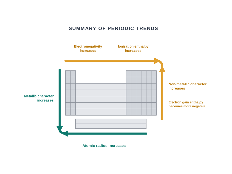
Fig. 3.8 – Summary of periodic trends in elements.
3.7.2 Periodic Trends in Chemical Properties
Most of the trends in chemical properties of elements — such as diagonal relationships, the inert pair effect, and the effects of lanthanoid contraction — will be dealt with alongside the discussion of each group in later chapters. In this section we shall study the periodicity of the valence state shown by elements, and the anomalous properties of the second-period elements (from lithium to fluorine).
Periodicity of Valence or Oxidation States
The valence is the most characteristic property of the elements, and it can be understood in terms of their electronic configurations. The valence of representative elements is usually (though not necessarily) equal to the number of electrons in the outermost orbitals, and/or equal to eight minus the number of outermost electrons, as shown below.
| Group | 1 | 2 | 13 | 14 | 15 | 16 | 17 | 18 |
|---|---|---|---|---|---|---|---|---|
| Number of valence electrons | 1 | 2 | 3 | 4 | 5 | 6 | 7 | 8 |
| Valence | 1 | 2 | 3 | 4 | 3, 5 | 2, 6 | 1, 7 | 0, 8 |
Nowadays, the term oxidation state is frequently used in place of valence. Consider the two oxygen-containing compounds \(\mathrm{OF_2}\) and \(\mathrm{Na_2O}\). The order of electronegativity among the three elements involved is F > O > Na.
In \(\mathrm{OF_2}\), each fluorine atom (outer configuration \(2s^2 2p^5\)) shares one electron with oxygen. Being the most electronegative element, fluorine is given the oxidation state –1. Since there are two fluorine atoms, oxygen (outer configuration \(2s^2 2p^4\)) shares two electrons and thereby exhibits an oxidation state of +2.
In \(\mathrm{Na_2O}\), oxygen, being more electronegative, accepts two electrons — one from each of the two sodium atoms — and thus shows an oxidation state of –2. Sodium (configuration \(3s^1\)) loses one electron to oxygen and is given an oxidation state of +1.
In this way, the oxidation state of an element in a particular compound can be defined as the charge acquired by its atom on the basis of electronegative consideration relative to the other atoms in the molecule.
Some periodic trends in the valence of elements, seen through the formulas of their hydrides and oxides, are shown in Table 3.9. Many elements also exhibit variable valence — this is particularly characteristic of the transition elements and the actinoids, which we shall study later.
Table 3.9 Periodic Trends in Valence of Elements as Shown by the Formulas of Their Compounds
| Group | 1 | 2 | 13 | 14 | 15 | 16 | 17 |
|---|---|---|---|---|---|---|---|
| Formula of hydride | \(\mathrm{LiH}\), \(\mathrm{NaH}\), \(\mathrm{KH}\) | \(\mathrm{CaH_2}\) | \(\mathrm{B_2H_6}\), \(\mathrm{AlH_3}\) | \(\mathrm{CH_4}\), \(\mathrm{SiH_4}\), \(\mathrm{GeH_4}\), \(\mathrm{SnH_4}\) | \(\mathrm{NH_3}\), \(\mathrm{PH_3}\), \(\mathrm{AsH_3}\) | \(\mathrm{H_2O}\), \(\mathrm{H_2S}\), \(\mathrm{H_2Se}\), \(\mathrm{H_2Te}\) | \(\mathrm{HF}\), \(\mathrm{HCl}\), \(\mathrm{HBr}\), \(\mathrm{HI}\) |
| Formula of oxide | \(\mathrm{Li_2O}\), \(\mathrm{Na_2O}\), \(\mathrm{K_2O}\) | \(\mathrm{MgO}\), \(\mathrm{CaO}\), \(\mathrm{SrO}\), \(\mathrm{BaO}\) | \(\mathrm{B_2O_3}\), \(\mathrm{Al_2O_3}\), \(\mathrm{Ga_2O_3}\), \(\mathrm{In_2O_3}\) | \(\mathrm{CO_2}\), \(\mathrm{SiO_2}\), \(\mathrm{GeO_2}\), \(\mathrm{SnO_2}\), \(\mathrm{PbO_2}\) | \(\mathrm{N_2O_3}\), \(\mathrm{N_2O_5}\), \(\mathrm{P_4O_6}\), \(\mathrm{P_4O_{10}}\), \(\mathrm{As_2O_3}\), \(\mathrm{As_2O_5}\), \(\mathrm{Sb_2O_3}\), \(\mathrm{Sb_2O_5}\), \(\mathrm{Bi_2O_3}\) | \(\mathrm{SO_3}\), \(\mathrm{SeO_3}\), \(\mathrm{TeO_3}\) | \(\mathrm{Cl_2O_7}\) |
Anomalous Properties of Second Period Elements
The first element of each of the groups 1 (lithium) and 2 (beryllium), and of the groups 13 to 17 (boron to fluorine), differs in many respects from the other members of its own group.
For example, lithium (unlike the other alkali metals) and beryllium (unlike the other alkaline earth metals) form compounds with pronounced covalent character, whereas the other members of these groups predominantly form ionic compounds. In fact, the behaviour of lithium and beryllium is more similar to that of the second element of the following group — that is, magnesium and aluminium, respectively. This kind of similarity is commonly referred to as a diagonal relationship in periodic properties, and it is reflected in the radii shown below.
| Property | Li | Be | B | Na | Mg | Al |
|---|---|---|---|---|---|---|
| Metallic radius M / pm | 152 | 111 | 88 | 186 | 160 | 143 |
| Ionic radius M⁺ / pm | 76 | 31 | – | 102 | 72 | – |
What are the reasons for the different chemical behaviour of the first member of a group in the s- and p-blocks, compared with the subsequent members? The anomalous behaviour is attributed to their small size, their large charge/radius ratio, and their high electronegativity.
In addition, the first member of a group has only four valence orbitals (2s and 2p) available for bonding, whereas the second member of the group has nine valence orbitals (3s, 3p, 3d). As a consequence, the maximum covalency of the first member of each group is limited to 4. For example, boron can only form \([\mathrm{BF_4}]^-\), whereas the other members of the group can expand their valence shell to accommodate more than four pairs of electrons — for instance, aluminium forms \([\mathrm{AlF_6}]^{3-}\).
Furthermore, the first member of the p-block elements displays a greater ability to form \(p\pi\)–\(p\pi\) multiple bonds — both to itself (for example, \(\mathrm{C=C}\), \(\mathrm{C\equiv C}\), \(\mathrm{N=N}\), \(\mathrm{N\equiv N}\)) and to other second-period elements (for example, \(\mathrm{C=O}\), \(\mathrm{C=N}\), \(\mathrm{C\equiv N}\), \(\mathrm{N=O}\)) — compared with the subsequent members of the same group.
3.7.3 Periodic Trends and Chemical Reactivity
We have now observed the periodic trends in certain fundamental properties — atomic and ionic radii, ionization enthalpy, electron gain enthalpy, and valence. We know by now that this periodicity is closely related to electronic configuration; indeed, all chemical and physical properties are a manifestation of the electronic configuration of elements. Let us now explore how these fundamental properties connect to chemical reactivity.
The atomic and ionic radii generally decrease across a period from left to right. As a consequence, the ionization enthalpies generally increase (with the exceptions outlined earlier), and the electron gain enthalpies become more negative across the period.
In other words, the ionization enthalpy of the element at the extreme left of a period is the smallest, and the electron gain enthalpy of the element at the extreme right is the most negative (noting that the noble gases, with completely filled shells, have rather positive electron gain enthalpies). This results in high chemical reactivity at the two extremes of a period, and the lowest reactivity in the centre.
Thus, the maximum chemical reactivity at the extreme left (among the alkali metals) is shown by the easy loss of an electron, leading to the formation of a cation. At the extreme right (among the halogens), the maximum reactivity is shown by the gain of an electron, forming an anion. This behaviour can be related to the reducing and oxidizing behaviour of the elements, which you will study later.
More directly, it can be related to the metallic and non-metallic character of the elements. The metallic character of an element, highest at the extreme left, decreases, while the non-metallic character increases, as we move from left to right across the period.
Reaction with Oxygen: the Nature of Oxides
The chemical reactivity of an element can be shown well by its reactions with oxygen and with the halogens. Here we shall consider the reaction with oxygen only. Elements at the two extremes of a period readily combine with oxygen to form oxides.
The normal oxide formed by the element at the extreme left is the most basic (for example, \(\mathrm{Na_2O}\)), whereas that formed by the element at the extreme right is the most acidic (for example, \(\mathrm{Cl_2O_7}\)). Oxides of elements in the centre are amphoteric (for example, \(\mathrm{Al_2O_3}\), \(\mathrm{As_2O_3}\)) or neutral (for example, CO, NO, \(\mathrm{N_2O}\)).
Reactivity Trends Down a Group and in the Transition Series
Among the transition metals (the 3d series), the change in atomic radii across the period is much smaller than that among the representative elements. The change in atomic radii is smaller still among the inner-transition metals (the 4f series). The ionization enthalpies of the transition metals are intermediate between those of the s- and p-blocks. As a consequence, they are less electropositive than the Group 1 and Group 2 metals.
In a group, the increase in atomic and ionic radii with increasing atomic number generally results in a gradual decrease in ionization enthalpies, and a regular decrease (with an exception in some third-period elements, as noted in the electron gain enthalpy discussion) in electron gain enthalpies for the main group elements.
Thus, the metallic character increases down a group and the non-metallic character decreases. This trend can be related to the reducing and oxidizing properties of the elements, which you will learn later. In the case of the transition elements, however, a reverse trend is observed, which can be explained in terms of atomic size and ionization enthalpy.
3.8 Summary
In this Chapter, you studied the development of the Periodic Law and the Periodic Table, and the periodic trends that follow from the electronic configurations of atoms. The key ideas are recapped below.
How the Periodic Table developed
- The classification of elements grew from the work of many scientists. The overall journey — from the first hints of a pattern to the modern law — is condensed in FC 3.3.
Flowchart
FC 3.3 – Development of the Periodic Table: Döbereiner’s Triads (middle element ≈ average of the other two) → Newlands’ Law of Octaves (every 8th element similar, valid up to Ca) → Meyer & Mendeleev (properties recur at regular intervals with atomic weight; Mendeleev leaves gaps and predicts new elements) → Moseley (atomic number is more fundamental than atomic weight) → Modern Periodic Law (properties are periodic functions of atomic number).
- Mendeleev’s Periodic Table was based on atomic masses.
- The Modern Periodic Table arranges the elements in order of their atomic numbers, in seven horizontal rows (periods) and eighteen vertical columns (groups or families).
- Atomic numbers increase consecutively along a period, and in a regular pattern down a group.
Groups, periods, and blocks
- Elements of the same group have similar valence shell electronic configurations, and therefore show similar chemical properties.
- Elements of the same period have a steadily increasing number of electrons from left to right, and therefore have different valencies.
- On the basis of the orbital being filled, four types of elements are recognised: s-block, p-block, d-block, and f-block elements.
- Hydrogen, with a single electron in the \(1s\) orbital, occupies a unique position and is placed separately at the top of the table.
Metals, non-metals, and metalloids
- Metals make up more than 78% of the known elements.
- Non-metals, located towards the top right of the table, number fewer than twenty.
- Elements at the borderline between metals and non-metals (e.g., Si, Ge, As) are called metalloids or semi-metals.
- Metallic character increases down a group and decreases from left to right across a period.
- Overall, the physical and chemical properties of elements vary periodically with their atomic numbers.
Periodic trends in properties
- Periodic trends are seen in atomic size, ionization enthalpy, electron gain enthalpy, electronegativity, and valence.
- Atomic radii decrease from left to right across a period and increase down a group.
- Ionization enthalpies generally increase across a period and decrease down a group; electronegativity follows a similar trend.
- Electron gain enthalpies, in general, become more negative across a period and less negative down a group.
- Valence shows periodicity: for representative elements, the valence is either equal to the number of outermost electrons or to eight minus that number.
Chemical reactivity and the nature of oxides
- Chemical reactivity is highest at the two extremes of a period and lowest in the centre.
- Reactivity at the left extreme comes from the ease of electron loss (low ionization enthalpy); at the right extreme it comes from the ease of electron gain.
- Highly reactive elements do not occur free in nature; they are usually found in the combined form.
- Oxides of the elements on the left are basic, those on the right are acidic, and those in the centre are amphoteric or neutral.
3.9 NCERT Questions
What is the basic theme of organisation in the periodic table?
Which important property did Mendeleev use to classify the elements in his periodic table, and did he stick to that?
What is the basic difference in approach between Mendeleev’s Periodic Law and the Modern Periodic Law?
On the basis of quantum numbers, justify that the sixth period of the periodic table should have 32 elements.
In terms of period and group, where would you locate the element with \(Z = 114\)?
Write the atomic number of the element present in the third period and seventeenth group of the periodic table.
Which element do you think would have been named by
- Lawrence Berkeley Laboratory,
- Seaborg’s group?
Why do elements in the same group have similar physical and chemical properties?
What does atomic radius and ionic radius really mean to you?
How do atomic radii vary in a period and in a group? How do you explain the variation?
What do you understand by isoelectronic species? Name a species that will be isoelectronic with each of the following atoms or ions:
- \(\mathrm{F^-}\)
- Ar
- \(\mathrm{Mg^{2+}}\)
- \(\mathrm{Rb^+}\).
Consider the following species: \(\mathrm{N^{3-}}\), \(\mathrm{O^{2-}}\), \(\mathrm{F^-}\), \(\mathrm{Na^+}\), \(\mathrm{Mg^{2+}}\) and \(\mathrm{Al^{3+}}\).
- What is common in them?
- Arrange them in the order of increasing ionic radii.
Explain why cations are smaller and anions larger in radii than their parent atoms.
What is the significance of the terms ‘isolated gaseous atom’ and ‘ground state’ while defining ionization enthalpy and electron gain enthalpy? (Hint: requirements for comparison purposes.)
The energy of an electron in the ground state of the hydrogen atom is \(-2.18\times10^{-18}\ \text{J}\). Calculate the ionization enthalpy of atomic hydrogen in terms of \(\text{J mol}^{-1}\). (Hint: apply the idea of the mole concept to derive the answer.)
Among the second-period elements, the actual ionization enthalpies are in the order Li < B < Be < C < O < N < F < Ne. Explain why
- Be has higher \(\Delta_i H\) than B, and
- O has lower \(\Delta_i H\) than N and F.
How would you explain the fact that the first ionization enthalpy of sodium is lower than that of magnesium, but its second ionization enthalpy is higher than that of magnesium?
What are the various factors due to which the ionization enthalpy of the main group elements tends to decrease down a group?
The first ionization enthalpy values (in \(\text{kJ mol}^{-1}\)) of Group 13 elements are:
| B | Al | Ga | In | Tl |
|---|---|---|---|---|
| 801 | 577 | 579 | 558 | 589 |
How would you explain this deviation from the general trend?
Which of the following pairs of elements would have a more negative electron gain enthalpy?
- O or F
- F or Cl.
Would you expect the second electron gain enthalpy of O to be positive, more negative, or less negative than the first? Justify your answer.
What is the basic difference between the terms electron gain enthalpy and electronegativity?
How would you react to the statement that the electronegativity of N on the Pauling scale is 3.0 in all nitrogen compounds?
Describe the theory associated with the radius of an atom as it
- gains an electron,
- loses an electron.
Would you expect the first ionization enthalpies for two isotopes of the same element to be the same or different? Justify your answer.
What are the major differences between metals and non-metals?
Use the periodic table to answer the following questions.
- Identify an element with five electrons in the outer subshell.
- Identify an element that would tend to lose two electrons.
- Identify an element that would tend to gain two electrons.
- Identify the group having metal, non-metal, liquid as well as gas at room temperature.
The increasing order of reactivity among Group 1 elements is Li < Na < K < Rb < Cs, whereas that among Group 17 elements is F > Cl > Br > I. Explain.
Write the general outer electronic configuration of s-, p-, d-, and f-block elements.
Assign the position of the element having outer electronic configuration
- \(ns^2np^4\) for \(n = 3\),
- \((n-1)d^2ns^2\) for \(n = 4\), and
- \((n-2)f^7(n-1)d^1ns^2\) for \(n = 6\), in the periodic table.
The first (\(\Delta_i H_1\)) and the second (\(\Delta_i H_2\)) ionization enthalpies (in \(\text{kJ mol}^{-1}\)) and the electron gain enthalpy (\(\Delta_{eg}H\), in \(\text{kJ mol}^{-1}\)) of a few elements are given below:
| Element | \(\Delta_i H_1\) | \(\Delta_i H_2\) | \(\Delta_{eg}H\) |
|---|---|---|---|
| I | 520 | 7300 | – 60 |
| II | 419 | 3051 | – 48 |
| III | 1681 | 3374 | – 328 |
| IV | 1008 | 1846 | – 295 |
| V | 2372 | 5251 | + 48 |
| VI | 738 | 1451 | – 40 |
Which of the above elements is likely to be: a. the least reactive element; b. the most reactive metal; c. the most reactive non-metal; d. the least reactive non-metal; e. the metal which can form a stable binary halide of the formula \(\mathrm{MX_2}\) (X = halogen); f. the metal which can form a predominantly stable covalent halide of the formula \(\mathrm{MX}\) (X = halogen)?
- Predict the formulas of the stable binary compounds that would be formed by the combination of the following pairs of elements.
- Lithium and oxygen
- Magnesium and nitrogen
- Aluminium and iodine
- Silicon and oxygen
- Phosphorus and fluorine
- Element 71 and fluorine.
- In the modern periodic table, the period indicates the value of:
- atomic number
- atomic mass
- principal quantum number
- azimuthal quantum number.
- Which of the following statements related to the modern periodic table is incorrect?
- The p-block has 6 columns, because a maximum of 6 electrons can occupy all the orbitals in a p-shell.
- The d-block has 8 columns, because a maximum of 8 electrons can occupy all the orbitals in a d-subshell.
- Each block contains a number of columns equal to the number of electrons that can occupy that subshell.
- The block indicates the value of the azimuthal quantum number (\(l\)) for the last subshell that received electrons in building up the electronic configuration.
- Anything that influences the valence electrons will affect the chemistry of the element. Which one of the following factors does not affect the valence shell?
- Valence principal quantum number (\(n\))
- Nuclear charge (\(Z\))
- Nuclear mass
- Number of core electrons.
- The size of the isoelectronic species \(\mathrm{F^-}\), Ne, and \(\mathrm{Na^+}\) is affected by:
- nuclear charge (\(Z\))
- valence principal quantum number (\(n\))
- electron–electron interaction in the outer orbitals
- none of the factors, because their size is the same.
- Which one of the following statements is incorrect in relation to ionization enthalpy?
- Ionization enthalpy increases for each successive electron.
- The greatest increase in ionization enthalpy is experienced on removal of an electron from the core noble-gas configuration.
- The end of valence electrons is marked by a big jump in ionization enthalpy.
- Removal of an electron from an orbital bearing a lower \(n\) value is easier than from an orbital having a higher \(n\) value.
- Considering the elements B, Al, Mg, and K, the correct order of their metallic character is:
- B > Al > Mg > K
- Al > Mg > B > K
- Mg > Al > K > B
- K > Mg > Al > B.
- Considering the elements B, C, N, F, and Si, the correct order of their non-metallic character is:
- B > C > Si > N > F
- Si > C > B > N > F
- F > N > C > B > Si
- F > N > C > Si > B.
- Considering the elements F, Cl, O, and N, the correct order of their chemical reactivity in terms of oxidizing property is:
- F > Cl > O > N
- F > O > Cl > N
- Cl > F > O > N
- O > F > N > Cl.
3.10 Check Your Concepts
- Match each scientist in Column I with the correct contribution in Column II.
| Column I | Column II |
|---|---|
| a. Döbereiner | i. Showed atomic number is more fundamental than atomic weight |
| b. Newlands | ii. Law of Triads |
| c. Mendeleev | iii. Placement of the actinoids below the lanthanoids |
| d. Moseley | iv. Law of Octaves |
| e. Seaborg | v. Left gaps and predicted eka-aluminium and eka-silicon |
Newlands’ Law of Octaves worked only for the lighter elements and broke down after calcium. Suggest a reason why an ordering rule based purely on a fixed repeat of eight could not hold for the heavier elements.
Assertion: When elements are arranged by atomic number, tellurium is correctly placed before iodine, even though iodine is lighter. Reason: The atomic number, not the atomic weight, is the true basis of periodicity. State whether the assertion and reason are correct, and whether the reason correctly explains the assertion.
Helium has the electronic configuration \(1s^2\), which would place it in the s-block. Give the reason why it is nevertheless positioned along with the Group 18 elements in the p-block.
Hydrogen is placed separately at the top of the Periodic Table rather than firmly inside Group 1. Give two reasons that justify this special treatment.
An element has the ground-state electronic configuration \([\mathrm{Ar}]\,3d^{10}4s^24p^3\). Identify its block, period, and group, and state whether it is a metal, non-metal, or metalloid.
Give reasons:
- transition metals commonly show variable oxidation states;
- many transition-metal compounds are coloured.
Explain why the second ionization enthalpy of an element is always greater than its first ionization enthalpy.
Arrange Na, Mg, and Al in order of increasing first ionization enthalpy, and explain why the value for Al does not simply continue the trend set by Na and Mg.
Explain, using size and charge/radius ratio, why lithium resembles magnesium (a diagonal relationship) more closely than it resembles sodium.
State two reasons why boron, the first member of Group 13, differs in its chemical behaviour from the other members of the group.
Assertion: The electron gain enthalpy of fluorine is less negative than that of chlorine. Reason: The added electron in fluorine enters a small \(n = 2\) shell where it suffers greater electron–electron repulsion. State whether the assertion and reason are correct, and whether the reason correctly explains the assertion.
Classify each of the following oxides as basic, acidic, amphoteric, or neutral, and justify each answer using the position of the element in the Periodic Table: \(\mathrm{Na_2O}\), \(\mathrm{CO_2}\), \(\mathrm{Al_2O_3}\), \(\mathrm{N_2O}\).
Complete and balance the following reactions, and state what each tells you about the nature of the oxide:
- \(\mathrm{K_2O} + \mathrm{H_2O} \rightarrow\)
- \(\mathrm{SO_3} + \mathrm{H_2O} \rightarrow\)
Explain why the electronegativity of an element is not a fixed constant, unlike its atomic number.
Arrange F, Cl, Br, and I in decreasing order of the magnitude of their electron gain enthalpy, and point out the one place where the trend does not follow the simple “decreases down the group” expectation.
3.11 Practice With Numericals
The energy required to remove the most loosely bound electron from a single gaseous lithium atom is \(8.64\times10^{-19}\ \text{J}\). Calculate the first ionization enthalpy of lithium in \(\text{kJ mol}^{-1}\). (Take \(N_A = 6.022\times10^{23}\ \text{mol}^{-1}\).)
The atomic weights of calcium and barium are 40 and 137, respectively. Using Döbereiner’s law of triads, predict the atomic weight of strontium, the middle member of this triad.
Calculate the percentage by mass of oxygen in aluminium oxide, \(\mathrm{Al_2O_3}\). (Atomic masses: Al = 27, O = 16.)
The first ionization enthalpy of magnesium is \(737\ \text{kJ mol}^{-1}\). Express this energy as the ionization energy per single magnesium atom, in joules. (Take \(N_A = 6.022\times10^{23}\ \text{mol}^{-1}\).)
Determine the number of electrons in each of the species \(\mathrm{S^{2-}}\), \(\mathrm{Cl^-}\), and \(\mathrm{K^+}\), and state whether the three are isoelectronic. (Atomic numbers: S = 16, Cl = 17, K = 19.)
The atomic (covalent) radius of bromine is 114 pm. Estimate the Br–Br bond length in a bromine molecule, \(\mathrm{Br_2}\).
Using the orbital-counting method, calculate the maximum number of elements that would be present in the seventh period of the Periodic Table if it were complete. (The orbitals filled across this period are \(7s\), \(5f\), \(6d\), and \(7p\).)
Calculate the percentage by mass of sodium in sodium oxide, \(\mathrm{Na_2O}\). (Atomic masses: Na = 23, O = 16.)