Chapter 6: Equilibrium
In the early 1900s, a hard question hung over farming and, quietly, over war. Crops need nitrogen to grow, yet the air above every field is almost four-fifths nitrogen gas that plants cannot use directly. The world was running low on natural nitrogen fertilisers, and chemists wondered: could nitrogen from the air be forced to combine with hydrogen to make ammonia, the raw material for fertilisers?
The German chemist Fritz Haber took up the challenge. He mixed nitrogen and hydrogen in a sealed vessel at high temperature and pressure and measured the ammonia formed at regular intervals. He noticed something strange. After a certain time, the amounts of nitrogen, hydrogen and ammonia stopped changing — yet plenty of nitrogen and hydrogen were still present. The reaction had not stopped; it had reached a balance. Ammonia was still forming, and at the very same instant ammonia was breaking apart, at exactly matching rates.
Working with the engineer Carl Bosch, Haber turned this balance into an industrial process that still feeds much of the world today. Their discovery rested entirely on one idea you are about to study: chemical equilibrium — a restless, two-way balance rather than a dead stop.
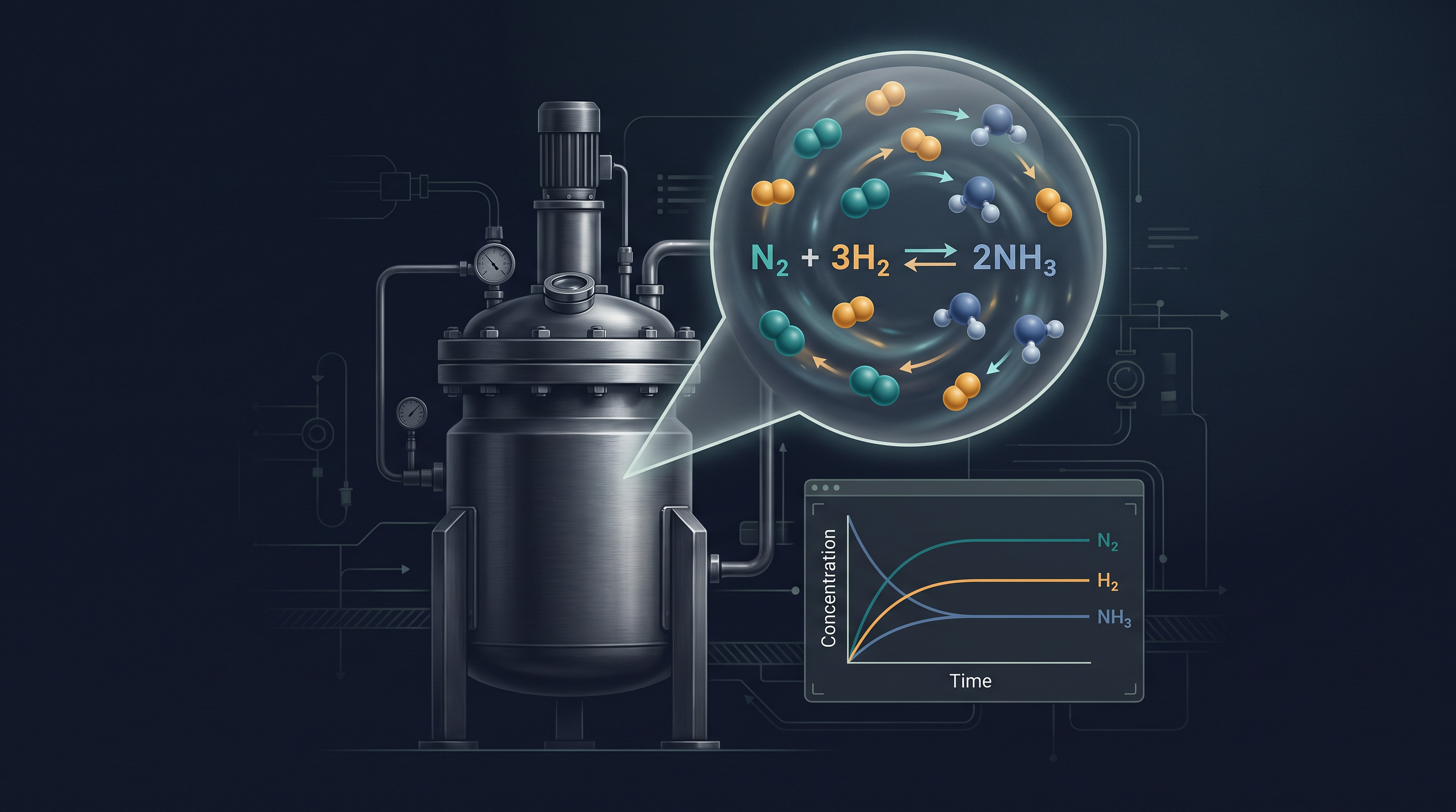
Fig. 6.0 – Dynamic equilibrium in the Haber process.
This chapter will give you the tools to reason your way to answers for each of these questions.
6.1 Equilibrium in Physical Processes
Before we study equilibrium in chemical reactions, it helps to watch it happen in simple physical changes that you already know — melting, boiling, sublimation and dissolving. In each of these, no new substance is made; only the physical state changes. Yet the same balancing act appears, and it is easier to picture here first.
The clearest examples are phase transformation processes — a substance moving from one physical state to another. The common ones are:
\[\mathrm{solid} \rightleftharpoons \mathrm{liquid}\] \[\mathrm{liquid} \rightleftharpoons \mathrm{gas}\] \[\mathrm{solid} \rightleftharpoons \mathrm{gas}\]
The double half-arrow (\(\rightleftharpoons\)) is important. It tells you the change is happening in both directions at once. Reading it left to right and right to left at the same time is the whole idea of equilibrium.
Why physical equilibria are worth studying first
In a physical process there is nothing to confuse us with a change of chemical identity. Water is water whether it is ice, liquid or vapour. So when we see the amounts of two phases become steady, we can be sure the steadiness comes from balance, not from a reaction using up the reactants. This makes physical processes an ideal training ground for the concept.
6.1.1 Solid-Liquid Equilibrium
Imagine a mixture of ice and water sealed inside a perfectly insulated thermos flask — one that allows no heat to pass between the contents and the surroundings — kept at 273 K and normal atmospheric pressure. If you watch the flask, nothing seems to happen. The mass of ice stays the same, the mass of water stays the same, and the temperature does not move.
But this stillness is only on the surface. At the boundary between ice and water there is intense activity. Water molecules keep colliding with the ice and sticking to it (freezing), while at the same time molecules of ice keep breaking away into the liquid (melting). Because these two opposite processes go on at exactly the same rate, the mass of ice and the mass of water do not change.
So the system is not “doing nothing.” It is in dynamic equilibrium — a balance kept alive by two opposing processes running at equal speed.
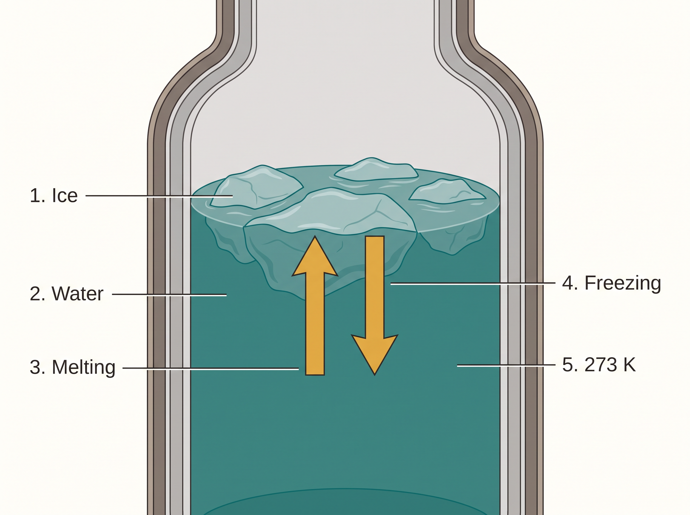
Fig. 6.1a – Solid-liquid equilibrium of ice and water.
There is a further point worth naming. Ice and water sit in balance only at one particular combination of temperature and pressure. For any pure substance at atmospheric pressure, the temperature at which its solid and liquid phases are in equilibrium has a special name.
From this we can draw two conclusions about the ice-water system:
First, both opposing processes (melting and freezing) go on together, at the same time. Second, they go on at the same rate, so the amounts of ice and water stay constant.
6.1.2 Liquid-Vapour Equilibrium
Now consider a liquid turning into vapour and back again. A neat way to observe this uses a closed, transparent box connected to a U-tube containing mercury — a manometer, which measures the pressure of gas inside the box. A manometer works simply: if the gas pressure rises, it pushes the mercury and the level in one limb climbs, so the height difference tells us the pressure.
First, a drying agent such as anhydrous calcium chloride (or phosphorus penta-oxide) is left in the box for a few hours to remove any moisture. The box is then tilted to remove the drying agent, and a watch glass (or petri dish) of water is quickly placed inside. The set-up is shown in Fig. 6.2.
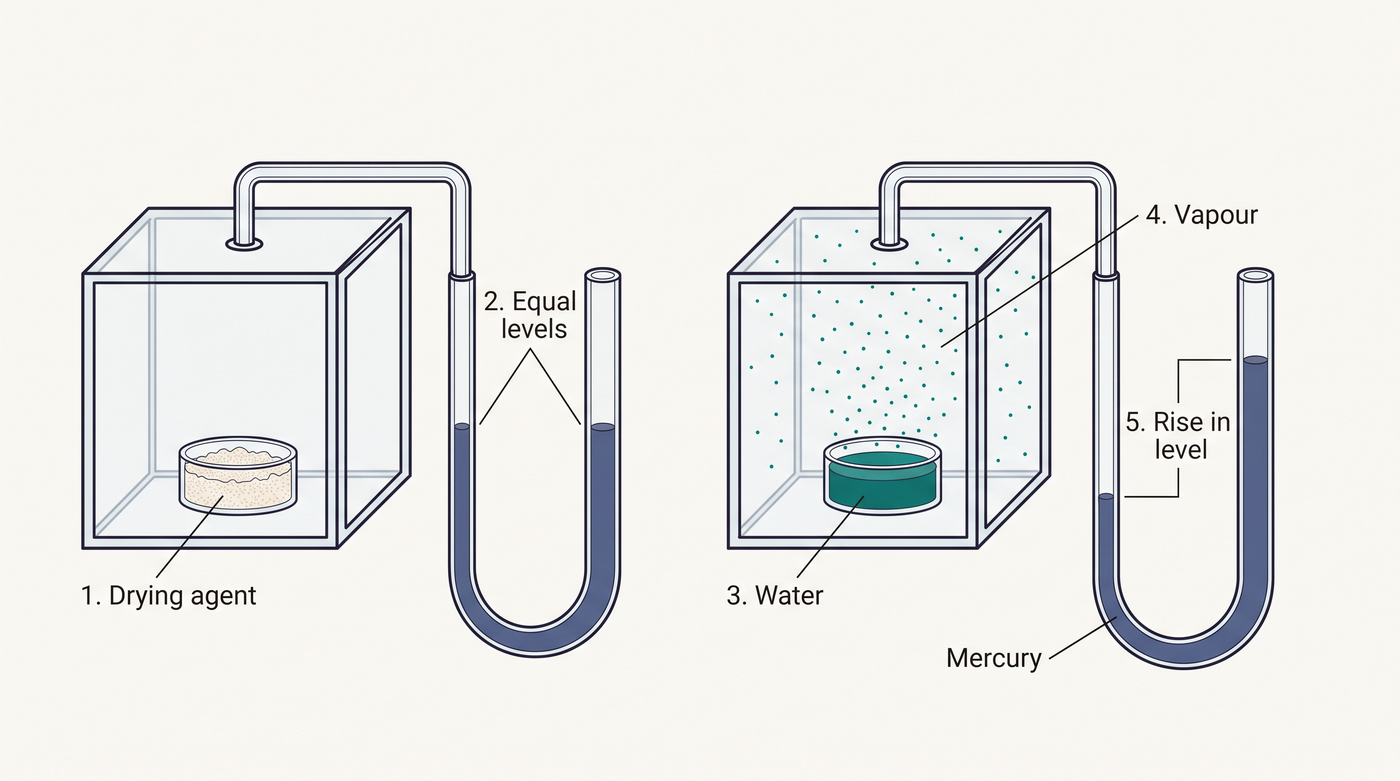
Fig. 6.2 – Measuring equilibrium vapour pressure of water.
Watch what happens. The mercury in the right limb of the manometer slowly rises and finally settles at a steady value — meaning the pressure inside the box rises and then becomes constant. At the same time, the volume of water in the watch glass falls a little and then stops falling.
Here is the reasoning behind these observations. At the start there was little or no water vapour in the box. As water evaporated, water molecules were added to the space above the liquid, so the pressure climbed. The rate of evaporation stays constant (it depends on temperature, which is fixed). But as more vapour builds up, more vapour molecules strike the liquid surface and return to it — so the rate of condensation keeps rising. Eventually condensation catches up with evaporation, and there is no further net loss of liquid:
\[\text{rate of evaporation} = \text{rate of condensation}\] \[\mathrm{H_2O}\text{(l)} \rightleftharpoons \mathrm{H_2O}\text{(vap)}\]
At this stage the pressure exerted by the vapour, at the given temperature, stays constant. This steady pressure has a name.
If the experiment is repeated with methyl alcohol, acetone and ether instead of water, each liquid settles at a different equilibrium vapour pressure at the same temperature. The liquid with the higher vapour pressure is more volatile — it escapes into vapour more readily — and therefore has a lower boiling point. This structure-property link matters: a liquid whose molecules are held together weakly evaporates easily, builds up a high vapour pressure, and boils at a lower temperature.
Open systems cannot reach equilibrium
There is an important condition hidden in all of this: the box must be closed. To see why, expose three watch glasses, each holding 1 mL of acetone, ethyl alcohol and water, to the open air in a warm room. In every case the liquid eventually disappears completely. How long it takes depends on (i) the nature of the liquid, (ii) the amount of liquid, and (iii) the temperature.
When the watch glass is open, the rate of evaporation stays constant, but the vapour molecules drift away into the huge volume of the room. Very few come back. So the rate of condensation stays far below the rate of evaporation, the two never become equal, and equilibrium is never reached. Equilibrium is impossible in an open system — the escaping molecules must be trapped for the reverse process to catch up.
The normal boiling point
Water and its vapour are in equilibrium at atmospheric pressure (1.013 bar) and 100 °C in a closed vessel — which is exactly why the boiling point of water is 100 °C at 1.013 bar. For any pure liquid, this defines another special temperature.
Because boiling depends on the surrounding pressure, the boiling point changes with altitude. High up on a mountain the atmospheric pressure is lower, so the boiling point of water falls below 100 °C — which is why cooking takes longer at high altitude.
6.1.3 Solid – Vapour Equilibrium
Some solids skip the liquid stage entirely and pass straight into vapour — a process called sublimation. Place solid iodine in a closed vessel and wait. The vessel slowly fills with violet vapour, and the colour deepens over time. After a while the intensity of the colour stops changing — equilibrium has been reached.
At this point solid iodine is subliming to give iodine vapour, and iodine vapour is condensing back to solid iodine, both at equal rates:
\[\mathrm{I_2}\text{(solid)} \rightleftharpoons \mathrm{I_2}\text{(vapour)}\]
The steady colour is the visible signal of the balance: as much vapour forms as returns to solid, so the amount of vapour stays constant.
Other substances show the same kind of solid-vapour equilibrium:
\[\mathrm{Camphor}\text{(solid)} \rightleftharpoons \mathrm{Camphor}\text{(vapour)}\] \[\mathrm{NH_4Cl}\text{(solid)} \rightleftharpoons \mathrm{NH_4Cl}\text{(vapour)}\]
6.1.4 Equilibrium Involving Dissolution of Solid or Gases in Liquids
Solids in liquids
You know from everyday experience that only a limited amount of salt or sugar will dissolve in a given amount of water at room temperature. If you make a thick sugar syrup by dissolving sugar at a high temperature and then cool it back down, sugar crystals separate out. A solution that can hold no more solute at a given temperature is called a saturated solution, and the concentration of solute in it depends on temperature.
In a saturated solution a dynamic equilibrium exists between the solute in the solid state and the solute in solution:
\[\mathrm{Sugar}\text{(solution)} \rightleftharpoons \mathrm{Sugar}\text{(solid)}\]
with
\[\text{rate of dissolution of sugar} = \text{rate of crystallisation of sugar}\]
How do we know both processes are really still going on, when the solution looks unchanging? The proof comes from a clever experiment using radioactive sugar — sugar whose molecules carry a radioactive marker that can be detected. Drop some radioactive sugar into a saturated solution of ordinary (non-radioactive) sugar. After some time, radioactivity shows up both in the solution and in the solid sugar at the bottom. Initially there was no radioactive sugar in the solution at all; the only way it could get there is if solid sugar keeps dissolving while dissolved sugar keeps crystallising, exchanging molecules between the two phases. The proportion of radioactive molecules in solution rises until it reaches a steady value — the mark of equilibrium.
Gases in liquids
Open a bottle of soda water and some of the dissolved carbon dioxide fizzes out at once. This happens because the solubility of carbon dioxide depends on the pressure of the gas above the liquid. Inside the sealed bottle there is an equilibrium between gaseous carbon dioxide and carbon dioxide dissolved in the liquid, held under pressure:
\[\mathrm{CO_2}\text{(gas)} \rightleftharpoons \mathrm{CO_2}\text{(in solution)}\]
This equilibrium is governed by Henry’s law.
The soda bottle is sealed under high gas pressure, so a lot of carbon dioxide stays dissolved. The moment you open it, the pressure above the liquid drops to the small partial pressure of carbon dioxide in the ordinary air. To reach the new, lower-pressure equilibrium, dissolved gas escapes — and if you leave the bottle open long enough, so much gas leaves that the drink goes “flat.”
Summing up the physical equilibria
These four physical systems can be generalised into a set of statements, which are collected in Table 6.1:
For a solid \(\rightleftharpoons\) liquid equilibrium, there is only one temperature (the melting point) at 1 atm (1.013 bar) at which the two phases can coexist. If no heat is exchanged with the surroundings, the mass of each phase stays constant.
For a liquid \(\rightleftharpoons\) vapour equilibrium, the vapour pressure is constant at a given temperature.
For dissolution of solids in liquids, the solubility is constant at a given temperature.
For dissolution of gases in liquids, the concentration of the gas in the liquid is proportional to the pressure of the gas over the liquid.
Table 6.1 Some Features of Physical Equilibria
| Process | Conclusion |
|---|---|
| Liquid \(\rightleftharpoons\) Vapour; \(\mathrm{H_2O}\text{(l)} \rightleftharpoons \mathrm{H_2O}\text{(g)}\) | \(p_{\mathrm{H_2O}}\) constant at a given temperature |
| Solid \(\rightleftharpoons\) Liquid; \(\mathrm{H_2O}\text{(s)} \rightleftharpoons \mathrm{H_2O}\text{(l)}\) | Melting point is fixed at constant pressure |
| Solute(s) \(\rightleftharpoons\) Solute (solution); \(\mathrm{Sugar}\text{(s)} \rightleftharpoons \mathrm{Sugar}\text{(solution)}\) | Concentration of solute in solution is constant at a given temperature |
| Gas(g) \(\rightleftharpoons\) Gas (aq); \(\mathrm{CO_2}\text{(g)} \rightleftharpoons \mathrm{CO_2}\text{(aq)}\) | \([\mathrm{gas(aq)}]/[\mathrm{gas(g)}]\) is constant at a given temperature; \([\mathrm{CO_2(aq)}]/[\mathrm{CO_2(g)}]\) is constant at a given temperature |
6.1.5 General Characteristics of Equilibria Involving Physical Processes
Looking back across all the physical processes above, five common features stand out for any system at equilibrium:
First, equilibrium is possible only in a closed system at a given temperature — otherwise, as we saw with the open watch glasses, the escaping molecules never return.
Second, both opposing processes occur at the same rate, giving a condition that is dynamic but stable.
Third, all measurable properties of the system remain constant — mass, pressure, colour intensity, concentration, and so on.
Fourth, when equilibrium is reached, it is marked by the constant value of one of its parameters at a given temperature (for example, the vapour pressure of a liquid, or the solubility of a solid). Table 6.1 lists such quantities.
Fifth, the magnitude of that constant quantity at any stage tells us how far the physical process has proceeded before reaching equilibrium.
6.2 Equilibrium in Chemical Processes – Dynamic Equilibrium
Just like the physical processes of the previous section, chemical reactions can also reach a state of equilibrium. These reactions run in both directions — forward and backward — and when the rates of the forward and reverse reactions become equal, the concentrations of reactants and products stop changing. That is the stage of chemical equilibrium.
The word dynamic is the key. The equilibrium is not a dead stop. It is made of a forward reaction, in which reactants give products, and a reverse reaction, in which products give back the original reactants — both going on together, endlessly.
Building up to the balance
To picture how this balance arises, take a general reversible reaction:
\[\mathrm{A} + \mathrm{B} \rightleftharpoons \mathrm{C} + \mathrm{D}\]
Suppose we start with only A and B. As time passes, products C and D pile up while reactants A and B are used up, as shown in Fig. 6.3.
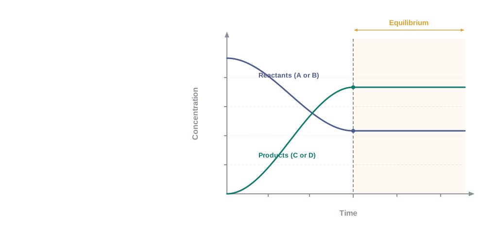
Fig. 6.3 – Concentration versus time for a reversible reaction.
This changing composition changes the two rates in opposite ways. As A and B get scarcer, the forward reaction slows down. As C and D build up, the reverse reaction speeds up. Sooner or later the two rates meet.
Eventually the forward and reverse reactions occur at the same rate, and the system reaches equilibrium. Notice that the concentrations then stay constant, but neither reaction has stopped.
An important consequence follows: the same equilibrium can be reached from either side. If instead we had started with only C and D — no A or B at all — the reverse reaction would run first, building up A and B until, once again, the two rates matched. The balance point does not care where you begin.
The deuterium experiment: proof that equilibrium is dynamic
How do we know the forward and reverse reactions are still running at equilibrium, rather than simply having stopped? The clearest proof comes from Haber’s synthesis of ammonia — the same reaction from our chapter opener.
In a series of experiments, Haber started with known amounts of dinitrogen and dihydrogen at high temperature and pressure, and measured the amount of ammonia at regular intervals, along with the leftover dihydrogen and dinitrogen. Fig. 6.4 (in the next section) shows that after a certain time the composition of the mixture stops changing even though some reactants are still present — a sure sign that equilibrium has been reached.
Now comes the elegant part. The synthesis is repeated under exactly the same conditions of partial pressure and temperature, but using \(\mathrm{D_2}\) (deuterium, a heavy form of hydrogen) in place of ordinary \(\mathrm{H_2}\). A mixture started with \(\mathrm{D_2}\) reaches equilibrium with the same overall composition — except that now \(\mathrm{D_2}\) and \(\mathrm{ND_3}\) are present instead of \(\mathrm{H_2}\) and \(\mathrm{NH_3}\).
Deuterium here acts as a tracer — a labelled atom we can follow. When the ordinary-hydrogen equilibrium mixture (\(\mathrm{H_2}\), \(\mathrm{N_2}\), \(\mathrm{NH_3}\)) and the deuterium equilibrium mixture (\(\mathrm{D_2}\), \(\mathrm{N_2}\), \(\mathrm{ND_3}\)) are mixed together and left for a while, the total amount of ammonia is unchanged. But when the mixture is analysed with a mass spectrometer — an instrument that sorts molecules by mass — something revealing shows up. The ammonia is now present in every mixed form: \(\mathrm{NH_3}\), \(\mathrm{NH_2D}\), \(\mathrm{NHD_2}\) and \(\mathrm{ND_3}\). The dihydrogen too appears as \(\mathrm{H_2}\), \(\mathrm{HD}\) and \(\mathrm{D_2}\).
The only way H and D atoms could get scrambled together like this is if the forward and reverse reactions kept running in the mixture, breaking molecules apart and rebuilding them in new combinations. Had the reaction simply stopped at equilibrium, no such mixing of isotopes could ever occur.
\[2\mathrm{NH_3}\text{(g)} \rightleftharpoons \mathrm{N_2}\text{(g)} + 3\mathrm{H_2}\text{(g)}\]
This is the definitive lesson: chemical reactions reach a state of dynamic equilibrium in which the rates of the forward and reverse reactions are equal and there is no net change in composition.
Reaching equilibrium from either side, again
The reversible reaction between dihydrogen and iodine gives another neat illustration. Consider:
\[\mathrm{H_2}\text{(g)} + \mathrm{I_2}\text{(g)} \rightleftharpoons 2\mathrm{HI}\text{(g)}\]
If we start with equal concentrations of \(\mathrm{H_2}\) and \(\mathrm{I_2}\), the reaction moves forward: \(\mathrm{H_2}\) and \(\mathrm{I_2}\) decrease while \(\mathrm{HI}\) increases, until all three become constant at equilibrium, as shown in Fig. 6.4.
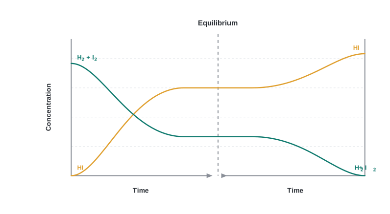
Fig. 6.4 – Reaching equilibrium from either direction.
We could equally well start with pure \(\mathrm{HI}\) alone and let the reverse reaction run: \(\mathrm{HI}\) decreases while \(\mathrm{H_2}\) and \(\mathrm{I_2}\) increase, again until all become constant. Provided the total number of H and I atoms in a given volume is the same, the very same equilibrium mixture is obtained whether we begin from pure reactants or pure product.
The same is true of the ammonia reaction. We can take \(\mathrm{H_2}\text{(g)}\) and \(\mathrm{N_2}\text{(g)}\) and make \(\mathrm{NH_3}\text{(g)}\), or take \(\mathrm{NH_3}\text{(g)}\) and decompose it back into \(\mathrm{N_2}\text{(g)}\) and \(\mathrm{H_2}\text{(g)}\):
\[\mathrm{N_2}\text{(g)} + 3\mathrm{H_2}\text{(g)} \rightleftharpoons 2\mathrm{NH_3}\text{(g)}\]
6.3 Law of Chemical Equilibrium and Equilibrium Constant
We now know that an equilibrium mixture is a mixture of reactants and products whose composition stops changing. But knowing that it stops is not enough. A chemist wants to answer sharper questions: What is the exact relationship between the concentrations of reactants and products at equilibrium? Can we predict the equilibrium concentrations from the starting ones? And which conditions can be adjusted to shift the balance toward more product? This last question is of huge practical value when choosing conditions for making industrial chemicals such as \(\mathrm{H_2}\), \(\mathrm{NH_3}\) and \(\mathrm{CaO}\).
The law of mass action
To answer these questions, consider once more a general reversible reaction:
\[\mathrm{A} + \mathrm{B} \rightleftharpoons \mathrm{C} + \mathrm{D}\]
where A and B are the reactants and C and D the products in the balanced equation. On the basis of experimental studies of many reversible reactions, the Norwegian chemists Cato Maximilian Guldberg and Peter Waage proposed in 1864 that the equilibrium concentrations are related by a simple equilibrium equation:
\[K_c = \frac{[\mathrm{C}][\mathrm{D}]}{[\mathrm{A}][\mathrm{B}]} \qquad (6.1)\]
Here \(K_c\) is the equilibrium constant, and the expression on the right is called the equilibrium constant expression. The square brackets stand for molar concentrations (in mol L⁻¹).
Finding the right expression: the H₂–I₂ data
Why is the equilibrium constant written with those particular powers? Guldberg and Waage’s expression was proposed from data, so let us follow the same evidence. Consider the reaction between gaseous \(\mathrm{H_2}\) and \(\mathrm{I_2}\) in a sealed vessel at 731 K:
\[\mathrm{H_2}\text{(g)} + \mathrm{I_2}\text{(g)} \rightleftharpoons 2\mathrm{HI}\text{(g)}\] \[1\ \text{mol} \qquad 1\ \text{mol} \qquad 2\ \text{mol}\]
Six sets of experiments were carried out. In the first four, the vessel started with only gaseous \(\mathrm{H_2}\) and \(\mathrm{I_2}\) (in different amounts); in the last two, it started with only \(\mathrm{HI}\). In every case the intensity of the purple colour (due to iodine) eventually became constant, showing equilibrium had been reached — from the forward direction in experiments 1–4 and from the reverse direction in experiments 5–6. The measured concentrations are given in Table 6.2.
Table 6.2 Initial and Equilibrium Concentrations of H₂, I₂ and HI
| Experiment number | Initial [H₂(g)] / mol L⁻¹ | Initial [I₂(g)] / mol L⁻¹ | Initial [HI(g)] / mol L⁻¹ | Equilibrium [H₂(g)] / mol L⁻¹ | Equilibrium [I₂(g)] / mol L⁻¹ | Equilibrium [HI(g)] / mol L⁻¹ |
|---|---|---|---|---|---|---|
| 1 | \(2.4 \times 10^{-2}\) | \(1.38 \times 10^{-2}\) | 0 | \(1.14 \times 10^{-2}\) | \(0.12 \times 10^{-2}\) | \(2.52 \times 10^{-2}\) |
| 2 | \(2.4 \times 10^{-2}\) | \(1.68 \times 10^{-2}\) | 0 | \(0.92 \times 10^{-2}\) | \(0.20 \times 10^{-2}\) | \(2.96 \times 10^{-2}\) |
| 3 | \(2.44 \times 10^{-2}\) | \(1.98 \times 10^{-2}\) | 0 | \(0.77 \times 10^{-2}\) | \(0.31 \times 10^{-2}\) | \(3.34 \times 10^{-2}\) |
| 4 | \(2.46 \times 10^{-2}\) | \(1.76 \times 10^{-2}\) | 0 | \(0.92 \times 10^{-2}\) | \(0.22 \times 10^{-2}\) | \(3.08 \times 10^{-2}\) |
| 5 | 0 | 0 | \(3.04 \times 10^{-2}\) | \(0.345 \times 10^{-2}\) | \(0.345 \times 10^{-2}\) | \(2.35 \times 10^{-2}\) |
| 6 | 0 | 0 | \(7.58 \times 10^{-2}\) | \(0.86 \times 10^{-2}\) | \(0.86 \times 10^{-2}\) | \(5.86 \times 10^{-2}\) |
Two patterns jump out. From experiments 1–4, the moles of dihydrogen reacted equal the moles of iodine reacted, and each equals half the moles of \(\mathrm{HI}\) formed — exactly what the balanced equation demands. From experiments 5–6, \([\mathrm{H_2(g)}]*{eq} = [\mathrm{I_2(g)}]*{eq}\), as expected when the mixture forms only from \(\mathrm{HI}\).
Now, which combination of these concentrations gives a constant? Try the simplest guess first:
\[\frac{[\mathrm{HI(g)}]*{eq}}{[\mathrm{H_2(g)}]*{eq}[\mathrm{I_2(g)}]_{eq}}\]
Plugging in the numbers (Table 6.3) shows this ratio is far from constant across the six experiments. But if instead we square the \(\mathrm{HI}\) term:
\[\frac{[\mathrm{HI(g)}]^2_{eq}}{[\mathrm{H_2(g)}]*{eq}[\mathrm{I_2(g)}]*{eq}}\]
the value comes out very nearly the same in all six cases.
Table 6.3 Expressions Involving the Equilibrium Concentrations for \(\mathrm{H_2}\text{(g)} + \mathrm{I_2}\text{(g)} \rightleftharpoons 2\mathrm{HI}\text{(g)}\)
| Experiment number | \(\dfrac{[\mathrm{HI(g)}]*{eq}}{[\mathrm{H_2(g)}]*{eq}[\mathrm{I_2(g)}]_{eq}}\) | \(\dfrac{[\mathrm{HI(g)}]^2_{eq}}{[\mathrm{H_2(g)}]*{eq}[\mathrm{I_2(g)}]*{eq}}\) |
|---|---|---|
| 1 | 1840 | 46.4 |
| 2 | 1610 | 47.6 |
| 3 | 1400 | 46.7 |
| 4 | 1520 | 46.9 |
| 5 | 1970 | 46.4 |
| 6 | 790 | 46.4 |
The lesson is written into the data: the power to which each concentration is raised is its stoichiometric coefficient in the balanced equation. Since \(\mathrm{HI}\) has a coefficient of 2, its concentration is squared. So for this reaction, following equation (6.1), the equilibrium constant is:
\[K_c = \frac{[\mathrm{HI(g)}]^2_{eq}}{[\mathrm{H_2(g)}]*{eq}[\mathrm{I_2(g)}]*{eq}} \qquad (6.2)\]
By convention, the subscript “eq” is dropped — it is understood that the concentrations in a \(K_c\) expression are always equilibrium values:
\[K_c = \frac{[\mathrm{HI(g)}]^2}{[\mathrm{H_2(g)}][\mathrm{I_2(g)}]} \qquad (6.3)\]
The subscript “c” reminds us that \(K_c\) is expressed using concentrations in mol L⁻¹.
We can now state the general law.
The general equilibrium constant expression
For a general reaction,
\[a\mathrm{A} + b\mathrm{B} \rightleftharpoons c\mathrm{C} + d\mathrm{D}\]
the equilibrium constant is:
\[K_c = \frac{[\mathrm{C}]^c[\mathrm{D}]^d}{[\mathrm{A}]^a[\mathrm{B}]^b} \qquad (6.4)\]
where \([\mathrm{A}]\), \([\mathrm{B}]\), \([\mathrm{C}]\) and \([\mathrm{D}]\) are equilibrium concentrations. As a worked pattern, the equilibrium constant for
\[4\mathrm{NH_3}\text{(g)} + 5\mathrm{O_2}\text{(g)} \rightleftharpoons 4\mathrm{NO}\text{(g)} + 6\mathrm{H_2O}\text{(g)}\]
is written as:
\[K_c = \frac{[\mathrm{NO}]^4[\mathrm{H_2O}]^6}{[\mathrm{NH_3}]^4[\mathrm{O_2}]^5}\]
Molar concentrations are shown by enclosing the species in square brackets, and these are understood to be equilibrium concentrations. When writing an equilibrium constant expression, the phase symbols (s, l, g) are generally left out.
How the equilibrium constant changes when the equation is rewritten
The value of \(K_c\) depends on exactly how the balanced equation is written. Three rules cover this, and they are exam favourites (often tested as “match the following” or “find the new K”).
Reversing the reaction. Take the forward reaction and its constant:
\[\mathrm{H_2}\text{(g)} + \mathrm{I_2}\text{(g)} \rightleftharpoons 2\mathrm{HI}\text{(g)} \qquad (6.5)\] \[K_c = \frac{[\mathrm{HI}]^2}{[\mathrm{H_2}][\mathrm{I_2}]} = x \qquad (6.6)\]
For the reverse reaction at the same temperature:
\[2\mathrm{HI}\text{(g)} \rightleftharpoons \mathrm{H_2}\text{(g)} + \mathrm{I_2}\text{(g)}\] \[K'_c = \frac{[\mathrm{H_2}][\mathrm{I_2}]}{[\mathrm{HI}]^2} = \frac{1}{x} = \frac{1}{K_c} \qquad (6.7)\]
So:
\[K'_c = \frac{1}{K_c} \qquad (6.8)\]
The equilibrium constant for the reverse reaction is simply the inverse of the constant for the forward reaction.
Multiplying the coefficients by a factor. If we halve the coefficients of reaction (6.5):
\[\tfrac{1}{2}\mathrm{H_2}\text{(g)} + \tfrac{1}{2}\mathrm{I_2}\text{(g)} \rightleftharpoons \mathrm{HI}\text{(g)} \qquad (6.9)\]
the new constant is:
\[K''_c = \frac{[\mathrm{HI}]}{[\mathrm{H_2}]^{1/2}[\mathrm{I_2}]^{1/2}} = \left{\frac{[\mathrm{HI}]^2}{[\mathrm{H_2}][\mathrm{I_2}]}\right}^{1/2} = x^{1/2} = K_c^{1/2} \qquad (6.10)\]
More generally, if reaction (6.5) is multiplied throughout by \(n\):
\[n\mathrm{H_2}\text{(g)} + n\mathrm{I_2}\text{(g)} \rightleftharpoons 2n\mathrm{HI}\text{(g)} \qquad (6.11)\]
then the equilibrium constant becomes \(K_c^{,n}\). These findings are summarised in Table 6.4.
Flowchart
FC 6.1 – How K changes when the equation is rewritten: original reaction (Kc) → reverse the reaction → new constant = 1/Kc; branch: multiply all coefficients by n → new constant = (Kc)ⁿ; special case n = ½ → new constant = (Kc)^½.
Table 6.4 Relations between Equilibrium Constants for a General Reaction and its Multiples
| Chemical equation | Equilibrium constant |
|---|---|
| \(a\mathrm{A} + b\mathrm{B} \rightleftharpoons c\mathrm{C} + d\mathrm{D}\) | \(K_c\) |
| \(c\mathrm{C} + d\mathrm{D} \rightleftharpoons a\mathrm{A} + b\mathrm{B}\) | \(K'_c = (1/K_c)\) |
| \(na\mathrm{A} + nb\mathrm{B} \rightleftharpoons nc\mathrm{C} + nd\mathrm{D}\) | \(K'''_c = (K_c^{,n})\) |
Because \(K_c\) and \(K'_c\) have different numerical values, it is essential to always state the exact form of the balanced equation when quoting the value of an equilibrium constant. A number like “\(K_c = 46.4\)” is meaningless unless the equation it belongs to is given.
6.4 Homogeneous Equilibria
An equilibrium is called homogeneous when all the reactants and products are present in the same phase. There is no boundary between a solid and a gas, or between a liquid and a solid — everything is mixed together as one uniform phase.
The ammonia synthesis is a good example: in
\[\mathrm{N_2}\text{(g)} + 3\mathrm{H_2}\text{(g)} \rightleftharpoons 2\mathrm{NH_3}\text{(g)}\]
every species is a gas, so reactants and products share the same gaseous phase. Reactions in solution can also be homogeneous, as in the ester hydrolysis
\[\mathrm{CH_3COOC_2H_5}\text{(aq)} + \mathrm{H_2O}\text{(l)} \rightleftharpoons \mathrm{CH_3COOH}\text{(aq)} + \mathrm{C_2H_5OH}\text{(aq)}\]
and the complex-forming reaction
\[\mathrm{Fe^{3+}}\text{(aq)} + \mathrm{SCN^{-}}\text{(aq)} \rightleftharpoons \mathrm{Fe(SCN)^{2+}}\text{(aq)}\]
where the reactants and products all stay in the same solution phase. We now look at how to write the equilibrium constant for such homogeneous reactions, especially the gaseous ones.
6.4.1 Equilibrium Constant in Gaseous Systems
So far we have written the equilibrium constant using molar concentrations, calling it \(K_c\). For reactions involving gases, though, it is often more convenient to work with partial pressures instead of concentrations — because the pressure of a gas is easy to measure directly. The partial pressure of a gas is the pressure that gas alone would exert if it occupied the whole container.
Linking pressure to concentration
To connect the two, we start from the ideal gas equation:
\[pV = nRT\]
Rearranging to bring the amount and volume together:
\[p = \frac{n}{V},RT\]
Here \(p\) is the pressure in Pa, \(n\) is the number of moles of gas, \(V\) is the volume in m³, and \(T\) is the temperature in kelvin. Now \(n/V\) is just the concentration of the gas (moles per unit volume). If we express concentration \(c\) in mol L⁻¹ (that is, mol dm⁻³) and \(p\) in bar, then:
\[p = cRT\]
which we can also write as \(p = [\text{gas}],RT\), using \(R = 0.0831\ \text{bar L mol}^{-1}\text{K}^{-1}\). So, at constant temperature, the pressure of a gas is directly proportional to its concentration:
\[p \propto [\text{gas}]\]
This single relationship is the bridge between \(K_p\) and \(K_c\).
A case where K_p equals K_c
Take the hydrogen–iodine reaction in equilibrium:
\[\mathrm{H_2}\text{(g)} + \mathrm{I_2}\text{(g)} \rightleftharpoons 2\mathrm{HI}\text{(g)}\]
We can write the equilibrium constant in terms of concentrations:
\[K_c = \frac{[\mathrm{HI(g)}]^2}{[\mathrm{H_2(g)}][\mathrm{I_2(g)}]}\]
or in terms of partial pressures:
\[K_p = \frac{(p_{\mathrm{HI}})^2}{(p_{\mathrm{H_2}})(p_{\mathrm{I_2}})} \qquad (6.12)\]
Since \(p = [\text{gas}],RT\) for each species:
\[p_{\mathrm{HI}} = [\mathrm{HI(g)}],RT, \qquad p_{\mathrm{I_2}} = [\mathrm{I_2(g)}],RT, \qquad p_{\mathrm{H_2}} = [\mathrm{H_2(g)}],RT\]
Substituting these into the \(K_p\) expression:
\[K_p = \frac{[\mathrm{HI(g)}]^2,(RT)^2}{[\mathrm{H_2(g)}],RT \cdot [\mathrm{I_2(g)}],RT} = \frac{[\mathrm{HI(g)}]^2}{[\mathrm{H_2(g)}][\mathrm{I_2(g)}]} = K_c \qquad (6.13)\]
The \(RT\) terms cancel exactly. Here \(K_p = K_c\) — but this happens only because the number of gas molecules is the same on both sides (2 on the left, 2 on the right).
The general relationship between K_p and K_c
When the number of gas molecules differs between the two sides, the \(RT\) terms do not fully cancel. Take ammonia synthesis:
\[\mathrm{N_2}\text{(g)} + 3\mathrm{H_2}\text{(g)} \rightleftharpoons 2\mathrm{NH_3}\text{(g)}\] \[K_p = \frac{(p_{\mathrm{NH_3}})^2}{(p_{\mathrm{N_2}})(p_{\mathrm{H_2}})^3}\]
Substituting \(p = [\text{gas}],RT\) for every species:
\[K_p = \frac{[\mathrm{NH_3(g)}]^2,(RT)^2}{[\mathrm{N_2(g)}],RT \cdot [\mathrm{H_2(g)}]^3,(RT)^3} = \frac{[\mathrm{NH_3(g)}]^2}{[\mathrm{N_2(g)}][\mathrm{H_2(g)}]^3},(RT)^{-2} = K_c,(RT)^{-2}\]
so
\[K_p = K_c,(RT)^{-2} \qquad (6.14)\]
The exponent \(-2\) appears because there are 4 gas molecules on the reactant side and 2 on the product side, a difference of \(2 - 4 = -2\). Generalising for
\[a\mathrm{A} + b\mathrm{B} \rightleftharpoons c\mathrm{C} + d\mathrm{D}\]
we substitute pressures for concentrations and collect the \(RT\) factors:
\[K_p = \frac{(p_C^c)(p_D^d)}{(p_A^a)(p_B^b)} = \frac{[\mathrm{C}]^c[\mathrm{D}]^d,(RT)^{(c+d)}}{[\mathrm{A}]^a[\mathrm{B}]^b,(RT)^{(a+b)}} = \frac{[\mathrm{C}]^c[\mathrm{D}]^d}{[\mathrm{A}]^a[\mathrm{B}]^b},(RT)^{(c+d)-(a+b)}\]
\[K_p = K_c,(RT)^{\Delta n} \qquad (6.15)\]
where
\[\Delta n = (\text{moles of gaseous products}) - (\text{moles of gaseous reactants})\]
in the balanced equation. This one formula handles every gaseous equilibrium. When \(\Delta n = 0\) (equal gas molecules on both sides), \((RT)^0 = 1\) and \(K_p = K_c\), exactly as we found for the \(\mathrm{H_2}\)–\(\mathrm{I_2}\) case.
An important practical note: when calculating \(K_p\), pressure must be expressed in bar, because the standard state for pressure is 1 bar. Recall from Chapter 1 that 1 pascal (Pa) \(= 1\ \text{N m}^{-2}\), and \(1\ \text{bar} = 10^5\ \text{Pa}\).
Values of \(K_p\) for a few selected reactions at different temperatures are listed in Table 6.5.
Table 6.5 Equilibrium Constants, \(K_p\), for a Few Selected Reactions
| Reaction | Temperature / K | \(K_p\) |
|---|---|---|
| \(\mathrm{N_2(g)} + 3\mathrm{H_2(g)} \rightleftharpoons 2\mathrm{NH_3}\) | 298 | \(6.8 \times 10^{5}\) |
| 400 | 41 | |
| 500 | \(3.6 \times 10^{-2}\) | |
| \(2\mathrm{SO_2(g)} + \mathrm{O_2(g)} \rightleftharpoons 2\mathrm{SO_3(g)}\) | 298 | \(4.0 \times 10^{24}\) |
| 500 | \(2.5 \times 10^{10}\) | |
| 700 | \(3.0 \times 10^{4}\) | |
| \(\mathrm{N_2O_4(g)} \rightleftharpoons 2\mathrm{NO_2(g)}\) | 298 | 0.98 |
| 400 | 47.9 | |
| 500 | 1700 |
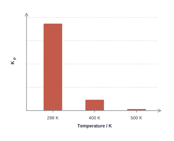
Fig. 6.5a – Effect of temperature on Kp for ammonia synthesis.
6.5 Heterogeneous Equilibria
In the last section every species shared a single phase. But many important equilibria involve more than one phase at once — a solid together with a gas, or a solid together with its solution. An equilibrium in a system having more than one phase is called a heterogeneous equilibrium.
A familiar example is the balance between liquid water and its vapour in a closed container:
\[\mathrm{H_2O}\text{(l)} \rightleftharpoons \mathrm{H_2O}\text{(g)}\]
Here there is a gas phase and a liquid phase — two phases, so the equilibrium is heterogeneous. In the same way, the balance between a solid and its saturated solution,
\[\mathrm{Ca(OH)_2}\text{(s)} + \text{(aq)} \rightleftharpoons \mathrm{Ca^{2+}}\text{(aq)} + 2\mathrm{OH^{-}}\text{(aq)}\]
involves a solid phase and a solution phase, and is again heterogeneous.
Why pure solids and liquids drop out of the expression
Heterogeneous equilibria often contain pure solids or pure liquids, and these can be handled with a helpful simplification. The molar concentration of a pure solid or a pure liquid is constant — it does not depend on how much of the substance is present. Think about it this way: a pure solid has a fixed density and a fixed molar mass, so the number of moles packed into each litre of the solid is always the same, whether you have a gram or a kilogram.
In symbols, if a substance X is a pure solid or liquid, then \([\mathrm{X(s)}]\) and \([\mathrm{X(l)}]\) are constant no matter how much X is taken. By contrast, \([\mathrm{X(g)}]\) and \([\mathrm{X(aq)}]\) do change as the amount of X in a given volume changes, so those cannot be treated as constant.
Because a constant can be absorbed into the equilibrium constant, the concentration terms for pure solids and pure liquids simply disappear from the expression.
The thermal decomposition of calcium carbonate
Let us take an interesting and industrially important case: the thermal decomposition (breakdown on heating) of calcium carbonate.
\[\mathrm{CaCO_3}\text{(s)} \xrightarrow{\ \Delta\ } \mathrm{CaO}\text{(s)} + \mathrm{CO_2}\text{(g)} \qquad (6.16)\]
Writing the full equilibrium constant from the stoichiometric equation:
\[K_c = \frac{[\mathrm{CaO(s)}][\mathrm{CO_2(g)}]}{[\mathrm{CaCO_3(s)}]}\]
Now both \([\mathrm{CaCO_3(s)}]\) and \([\mathrm{CaO(s)}]\) are pure solids, so both are constant. Absorbing these constants into a modified equilibrium constant leaves only the gas term:
\[K'_c = [\mathrm{CO_2(g)}] \qquad (6.17)\]
or, in terms of partial pressure:
\[K_p = p_{\mathrm{CO_2}} \qquad (6.18)\]
This is a striking result. It says that at any given temperature, there is a fixed concentration (or pressure) of \(\mathrm{CO_2}\) in equilibrium with solid \(\mathrm{CaCO_3}\) and solid \(\mathrm{CaO}\) — regardless of how much of the two solids is present. Experiment confirms it: at 1100 K, the pressure of \(\mathrm{CO_2}\) in equilibrium with \(\mathrm{CaCO_3(s)}\) and \(\mathrm{CaO(s)}\) is \(2.0 \times 10^5\ \text{Pa}\). Therefore the equilibrium constant at 1100 K is:
\[K_p = p_{\mathrm{CO_2}} = \frac{2 \times 10^5\ \text{Pa}}{10^5\ \text{Pa}} = 2.00\]
(dividing by the standard pressure of \(10^5\) Pa = 1 bar to get a pure number).
Another heterogeneous case: the Mond process
A second example is the equilibrium between nickel, carbon monoxide and nickel carbonyl, which is used in purifying nickel:
\[\mathrm{Ni}\text{(s)} + 4\mathrm{CO}\text{(g)} \rightleftharpoons \mathrm{Ni(CO)_4}\text{(g)}\]
Nickel is a pure solid, so its concentration is constant and drops out. The equilibrium constant contains only the gases:
\[K_c = \frac{[\mathrm{Ni(CO)_4}]}{[\mathrm{CO}]^4}\]
It must be remembered that for a heterogeneous equilibrium to exist, the pure solids or liquids must be present (however small the amount), even though their concentrations or partial pressures do not appear in the equilibrium constant. As one more illustration, in the reaction
\[\mathrm{Ag_2O}\text{(s)} + 2\mathrm{HNO_3}\text{(aq)} \rightleftharpoons 2\mathrm{AgNO_3}\text{(aq)} + \mathrm{H_2O}\text{(l)}\]
the pure solid \(\mathrm{Ag_2O}\) and the pure liquid \(\mathrm{H_2O}\) are both left out, giving:
\[K_c = \frac{[\mathrm{AgNO_3}]^2}{[\mathrm{HNO_3}]^2}\]
Units of Equilibrium Constant
The value of \(K_c\) is found by substituting concentration terms in mol L⁻¹, and \(K_p\) by substituting partial pressures in Pa, kPa, bar or atm. This gives \(K\) units based on molarity or pressure — unless the exponents in the numerator and denominator are equal, in which case the units cancel and \(K\) has no unit.
For example, for \(\mathrm{H_2}\text{(g)} + \mathrm{I_2}\text{(g)} \rightleftharpoons 2\mathrm{HI}\), there are two “concentration units” on top and two on the bottom, so \(K_c\) and \(K_p\) have no unit. But for \(\mathrm{N_2O_4}\text{(g)} \rightleftharpoons 2\mathrm{NO_2}\text{(g)}\), there are two units on top and one on the bottom, so \(K_c\) has unit mol L⁻¹ and \(K_p\) has unit bar.
There is a cleaner way to think about this. Equilibrium constants can be treated as dimensionless if we express every concentration and pressure relative to its standard state. For a pure gas the standard state is 1 bar, so a pressure of 4 bar is written as \(4\ \text{bar}/1\ \text{bar} = 4\), a pure number. The standard state (\(c_0\)) for a solute is a 1 molar solution, and all concentrations can be measured against it. The numerical value of the equilibrium constant depends on the standard state chosen. In this dimensionless system, both \(K_p\) and \(K_c\) are pure numbers, but they still have different numerical values because their standard states are different.
6.6 Applications of Equilibrium Constants
Now that we can write and calculate an equilibrium constant, what can we actually do with it? Before listing the applications, let us gather the key features of equilibrium constants that make them useful:
First, the equilibrium constant expression applies only when the concentrations of reactants and products have reached their constant equilibrium values.
Second, the value of the equilibrium constant is independent of the initial concentrations of reactants and products — you reach the same \(K\) from any starting mixture.
Third, the equilibrium constant is temperature dependent: it has one unique value for a particular reaction (written as a balanced equation) at a given temperature.
Fourth, the equilibrium constant for the reverse reaction is the inverse of that for the forward reaction.
Fifth, the equilibrium constant \(K\) for a reaction is related to the constant of a reaction whose equation is obtained by multiplying or dividing the original equation by a small integer (as we saw in Table 6.4).
With these in mind, the equilibrium constant lets us do three valuable things: predict the extent of a reaction from its magnitude, predict the direction in which a reaction will move, and calculate equilibrium concentrations. We take these in turn.
6.6.1 Predicting the Extent of a Reaction
The numerical value of the equilibrium constant tells us how far a reaction goes — how much product forms relative to reactant — before balance is reached. One caution first: the equilibrium constant says nothing about the rate at which equilibrium is reached. A reaction can have a huge \(K\) yet be painfully slow, or a small \(K\) yet be fast. Extent and speed are separate questions.
Why does the magnitude of \(K\) measure extent? Because \(K_c\) (or \(K_p\)) has products in the numerator and reactants in the denominator. So a large \(K\) means a large concentration of products relative to reactants — the reaction has gone far toward completion. A small \(K\) means the reactants dominate — the reaction has barely proceeded.
We can make three broad generalisations about the composition of equilibrium mixtures:
When \(K_c > 10^3\), products predominate over reactants. If \(K_c\) is very large, the reaction proceeds nearly to completion. Examples:
The reaction of \(\mathrm{H_2}\) with \(\mathrm{O_2}\) at 500 K has a very large equilibrium constant, \(K_c = 2.4 \times 10^{47}\).
\(\mathrm{H_2}\text{(g)} + \mathrm{Cl_2}\text{(g)} \rightleftharpoons 2\mathrm{HCl}\text{(g)}\) at 300 K has \(K_c = 4.0 \times 10^{31}\).
\(\mathrm{H_2}\text{(g)} + \mathrm{Br_2}\text{(g)} \rightleftharpoons 2\mathrm{HBr}\text{(g)}\) at 300 K has \(K_c = 5.4 \times 10^{18}\).
When \(K_c < 10^{-3}\), reactants predominate over products. If \(K_c\) is very small, the reaction hardly proceeds. Examples:
The decomposition of \(\mathrm{H_2O}\) into \(\mathrm{H_2}\) and \(\mathrm{O_2}\) at 500 K has a very small equilibrium constant, \(K_c = 4.1 \times 10^{-48}\).
\(\mathrm{N_2}\text{(g)} + \mathrm{O_2}\text{(g)} \rightleftharpoons 2\mathrm{NO}\text{(g)}\) at 298 K has \(K_c = 4.8 \times 10^{-31}\).
When \(K_c\) lies between \(10^{-3}\) and \(10^3\), appreciable concentrations of both reactants and products are present. Examples:
For the reaction of \(\mathrm{H_2}\) with \(\mathrm{I_2}\) to give \(\mathrm{HI}\), \(K_c = 57.0\) at 700 K.
The gas-phase decomposition of \(\mathrm{N_2O_4}\) to \(\mathrm{NO_2}\) has \(K_c = 4.64 \times 10^{-3}\) at 25 °C — neither too small nor too large — so equilibrium mixtures contain appreciable amounts of both \(\mathrm{N_2O_4}\) and \(\mathrm{NO_2}\).
These generalisations are illustrated in Fig. 6.6.
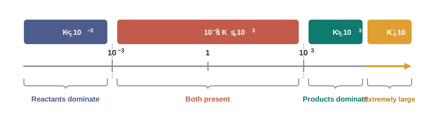
Fig. 6.6 – Predicting the extent of reaction from Kc.
6.6.2 Predicting the Direction of the Reaction
Suppose a reaction mixture is not at equilibrium. Which way will it move — forward or backward — to get there? To answer this we use the reaction quotient \(Q\).
The reaction quotient has exactly the same form as the equilibrium constant, except that the concentrations used are not necessarily equilibrium values — they are whatever the concentrations happen to be at some arbitrary moment. We write \(Q_c\) when using molar concentrations and \(Q_p\) when using partial pressures. For a general reaction:
\[a\mathrm{A} + b\mathrm{B} \rightleftharpoons c\mathrm{C} + d\mathrm{D} \qquad (6.19)\] \[Q_c = \frac{[\mathrm{C}]^c[\mathrm{D}]^d}{[\mathrm{A}]^a[\mathrm{B}]^b} \qquad (6.20)\]
The trick is to compare \(Q_c\) with \(K_c\):
If \(Q_c > K_c\), the reaction proceeds in the direction of the reactants (the reverse reaction).
If \(Q_c < K_c\), the reaction proceeds in the direction of the products (the forward reaction).
If \(Q_c = K_c\), the reaction mixture is already at equilibrium.
Why does this work? \(Q_c\) tells us the current ratio of products to reactants. If \(Q_c\) is smaller than \(K_c\), there are too few products, so the forward reaction runs to build them up. If \(Q_c\) is larger than \(K_c\), there are too many products, so the reverse reaction runs to consume them. Either way, the reaction moves until \(Q_c\) climbs or falls to equal \(K_c\).
A worked illustration makes this concrete. Consider the gaseous reaction of \(\mathrm{H_2}\) with \(\mathrm{I_2}\):
\[\mathrm{H_2}\text{(g)} + \mathrm{I_2}\text{(g)} \rightleftharpoons 2\mathrm{HI}\text{(g)}; \qquad K_c = 57.0\ \text{at}\ 700\ \text{K}\]
Suppose at some time \(t\) the molar concentrations are \([\mathrm{H_2}]_t = 0.10\ \text{M}\), \([\mathrm{I_2}]_t = 0.20\ \text{M}\) and \([\mathrm{HI}]_t = 0.40\ \text{M}\) (the subscript \(t\) means these were measured at an arbitrary time, not necessarily at equilibrium). The reaction quotient is:
\[Q_c = \frac{[\mathrm{HI}]_t^2}{[\mathrm{H_2}]_t[\mathrm{I_2}]_t} = \frac{(0.40)^2}{(0.10)(0.20)} = 8.0\]
Here \(Q_c = 8.0\) does not equal \(K_c = 57.0\), so the mixture is not at equilibrium. Since \(Q_c < K_c\), more \(\mathrm{H_2}\) and \(\mathrm{I_2}\) will react to form more \(\mathrm{HI}\), and their concentrations will change until \(Q_c = K_c\).
These generalisations about direction are shown in Fig. 6.7.
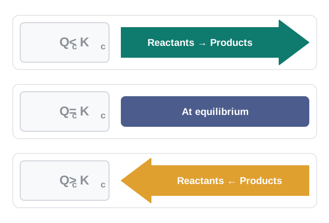
Fig. 6.7 – Predicting reaction direction using the reaction quotient.
Flowchart
FC 6.2 – Predicting reaction direction: compute Q_c from current concentrations → compare with K_c → if Q_c < K_c, net reaction goes left to right (forward); if Q_c > K_c, net reaction goes right to left (reverse); if Q_c = K_c, no net reaction (already at equilibrium).
6.6.3 Calculating Equilibrium Concentrations
The third application is the most practical for problem-solving: given the initial concentrations and the value of \(K\), find the equilibrium concentrations. A reliable five-step method handles almost every such problem.
Step 1. Write the balanced equation for the reaction.
Step 2. Under the balanced equation, make a table listing, for each substance: (a) the initial concentration, (b) the change in concentration on going to equilibrium, and (c) the equilibrium concentration. In building this table, define \(x\) as the concentration (mol L⁻¹) of one substance that reacts on going to equilibrium, then use the reaction stoichiometry to write the other concentrations in terms of \(x\).
Step 3. Substitute the equilibrium concentrations into the equilibrium constant expression and solve for \(x\). If a quadratic equation appears, choose the root that makes chemical sense (concentrations cannot be negative or exceed the initial amounts).
Step 4. Calculate the equilibrium concentrations from the value of \(x\).
Step 5. Check the results by substituting them back into the equilibrium constant expression.
This “ICE table” method (Initial, Change, Equilibrium) is worth mastering — most numerical equilibrium problems in board and entrance exams follow it.
Flowchart
FC 6.3 – Five-step method for equilibrium concentrations: write balanced equation → build initial/change/equilibrium table in terms of x → substitute into K expression and solve for x (pick the chemically sensible root) → compute equilibrium concentrations → check by back-substitution into K.
6.7 Relationship between Equilibrium Constant K, Reaction Quotient Q and Gibbs Energy G
We have treated the equilibrium constant as an experimental quantity — something we measure. But \(K\) is not just an observed number; it is deeply tied to the thermodynamics of a reaction. The value of \(K_c\) does not depend on the rate of the reaction; it depends instead on the change in Gibbs energy, \(\Delta G\), which you met in Unit 5.
Gibbs energy and the direction of a reaction
The Gibbs energy change of a reaction tells us whether it can happen on its own. Recall three cases:
If \(\Delta G\) is negative, the reaction is spontaneous and proceeds in the forward direction.
If \(\Delta G\) is positive, the reaction is non-spontaneous in the forward direction. Instead, the reverse reaction would have a negative \(\Delta G\), so the products of the forward reaction tend to convert back to reactants.
If \(\Delta G\) is zero, the reaction has reached equilibrium — there is no free energy left to drive it in either direction.
The key equation
The thermodynamic view of equilibrium is captured in one equation:
\[\Delta G = \Delta G^\circ + RT\ln Q \qquad (6.21)\]
where \(\Delta G^\circ\) is the standard Gibbs energy change (the value when all species are in their standard states), \(R\) is the gas constant, \(T\) is the temperature in kelvin, and \(Q\) is the reaction quotient. The logarithm appears here because Gibbs energy depends on the ratio of product to reactant activities, and thermodynamics links free energy to the natural logarithm of that ratio — a relationship carried over from Unit 5.
At equilibrium, two things are true at once: \(\Delta G = 0\) and \(Q = K_c\). Substituting these into equation (6.21):
\[\Delta G = \Delta G^\circ + RT\ln K = 0\]
which rearranges to:
\[\Delta G^\circ = -RT\ln K \qquad (6.22)\]
or equivalently:
\[\ln K = -\frac{\Delta G^\circ}{RT}\]
Taking the antilogarithm of both sides gives a form that is often more convenient:
\[K = e^{-\Delta G^\circ/RT} \qquad (6.23)\]
This equation is powerful: it means we can find the equilibrium constant from a thermodynamic quantity, and vice versa. It also lets us interpret the sign of \(\Delta G^\circ\) in terms of how far a reaction goes.
Interpreting the sign of ΔG°
Using equation (6.23), the spontaneity of a reaction can be read straight from the value of \(\Delta G^\circ\):
If \(\Delta G^\circ < 0\), then \(-\Delta G^\circ/RT\) is positive, so \(e^{-\Delta G^\circ/RT} > 1\), making \(K > 1\). This implies a spontaneous reaction — one that proceeds forward so far that products predominate.
If \(\Delta G^\circ > 0\), then \(-\Delta G^\circ/RT\) is negative, so \(e^{-\Delta G^\circ/RT} < 1\), making \(K < 1\). This implies a non-spontaneous reaction — one that proceeds forward to such a small degree that only a tiny amount of product forms.
6.8 Factors Affecting Equilibria
One of the principal goals of chemical synthesis is to convert as much reactant into product as possible while spending as little energy as possible. In practice, that means getting the maximum yield of product under mild temperature and pressure conditions. When a reaction does not obligingly do this on its own, the experimental conditions must be adjusted.
The Haber process is the perfect illustration. In synthesising ammonia from \(\mathrm{N_2}\) and \(\mathrm{H_2}\), the choice of conditions is of real economic importance — the annual world production of ammonia is about a hundred million tonnes, used mainly as fertiliser. Getting the conditions right is worth a great deal.
Disturbing a system at equilibrium
We have seen that \(K_c\) is independent of the initial concentrations. But if a system already at equilibrium is disturbed — by changing the concentration of one of the reacting substances — it is no longer at equilibrium. A net reaction then takes place in some direction until the system settles into equilibrium once again. Changing the temperature or pressure can also alter the equilibrium.
To decide which way a disturbed system will move — that is, to make a qualitative prediction about the effect of a change in conditions — we use Le Chatelier’s principle.
In plain language: the system pushes back. Disturb it, and it shifts in whichever direction partially undoes the disturbance. We now examine the individual factors that can influence equilibrium.
6.8.1 Effect of Concentration Change
When equilibrium is disturbed by adding or removing a reactant or product, Le Chatelier’s principle predicts that:
The concentration stress of an added reactant/product is relieved by a net reaction in the direction that consumes the added substance.
The concentration stress of a removed reactant/product is relieved by a net reaction in the direction that replenishes the removed substance.
Or, put another way: when the concentration of any of the reactants or products in a reaction at equilibrium is changed, the composition of the equilibrium mixture changes so as to minimize the effect of the concentration change.
Take the familiar reaction:
\[\mathrm{H_2}\text{(g)} + \mathrm{I_2}\text{(g)} \rightleftharpoons 2\mathrm{HI}\text{(g)}\]
If \(\mathrm{H_2}\) is added to the mixture at equilibrium, the equilibrium is disturbed. To restore it, the reaction proceeds in the direction that consumes \(\mathrm{H_2}\) — that is, more \(\mathrm{H_2}\) and \(\mathrm{I_2}\) react to form \(\mathrm{HI}\), and the equilibrium shifts to the right (forward), as shown in Fig. 6.8. Le Chatelier’s principle implies that a new equilibrium is set up in which the concentration of the added substance is less than it was immediately after the addition, but more than it was in the original mixture. The system partially — not completely — undoes the change.
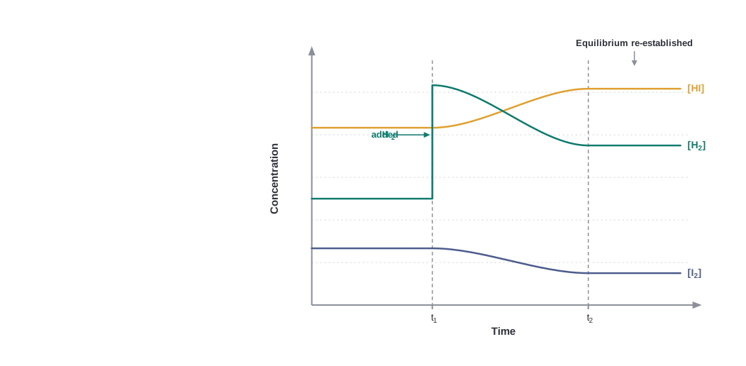
Fig. 6.8 – Effect of adding H₂ on the equilibrium mixture.
The same point can be explained using the reaction quotient:
\[Q_c = \frac{[\mathrm{HI}]^2}{[\mathrm{H_2}][\mathrm{I_2}]}\]
Adding hydrogen at equilibrium increases the denominator, so \(Q_c\) becomes less than \(K_c\). As we learned in Section 6.6.2, when \(Q_c < K_c\) the reaction moves forward — which is exactly what Le Chatelier’s principle predicted. The two approaches always agree; Le Chatelier is the quick qualitative rule, \(Q\) versus \(K\) is the quantitative reasoning behind it.
Similarly, removing a product boosts the forward reaction and increases the yield of products. This has enormous commercial value in reactions where the product is a gas or a volatile substance. In the manufacture of ammonia, the ammonia is liquefied and removed from the reaction mixture, so the reaction keeps moving forward. In the large-scale production of \(\mathrm{CaO}\) (an important building material) from \(\mathrm{CaCO_3}\), the constant removal of \(\mathrm{CO_2}\) from the kiln drives the reaction to completion. In terms of \(Q\): continuous removal of a product keeps \(Q_c\) permanently below \(K_c\), so the reaction never stops moving forward.
Effect of Concentration – An experiment
This shifting can be seen with a colourful reaction:
\[\mathrm{Fe^{3+}}\text{(aq)} + \mathrm{SCN^{-}}\text{(aq)} \rightleftharpoons \mathrm{[\text{Fe(SCN)}]^{2+}}\text{(aq)} \qquad (6.24)\] \[\text{yellow} \qquad \text{colourless} \qquad \text{deep red}\]
with
\[K_c = \frac{[\mathrm{Fe(SCN)^{2+}}\text{(aq)}]}{[\mathrm{Fe^{3+}}\text{(aq)}][\mathrm{SCN^{-}}\text{(aq)}]} \qquad (6.25)\]
Adding two drops of 0.002 M potassium thiocyanate solution to 1 mL of 0.2 M iron(III) nitrate solution produces a reddish colour, due to the formation of \(\mathrm{[\text{Fe(SCN)}]^{2+}}\). The intensity of the red colour becomes constant on attaining equilibrium. Because the intensity of the colour tracks the concentration of the deep-red complex, the eye can follow the shift directly.
This equilibrium can be pushed either way, depending on whether we add a reactant or a product. To shift it backward, we add reagents that remove \(\mathrm{Fe^{3+}}\) or \(\mathrm{SCN^{-}}\) ions:
Oxalic acid (\(\mathrm{H_2C_2O_4}\)) reacts with \(\mathrm{Fe^{3+}}\) ions to form the stable complex ion \(\mathrm{[\text{Fe}(C_2O_4)_3]^{3-}}\), thereby decreasing the concentration of free \(\mathrm{Fe^{3+}}\)(aq). By Le Chatelier’s principle, the stress of removed \(\mathrm{Fe^{3+}}\) is relieved by dissociation of \(\mathrm{[\text{Fe(SCN)}]^{2+}}\) to replenish the \(\mathrm{Fe^{3+}}\) ions. Because the concentration of \(\mathrm{[\text{Fe(SCN)}]^{2+}}\) falls, the intensity of the red colour decreases.
Adding aqueous \(\mathrm{HgCl_2}\) also fades the red colour, because \(\mathrm{Hg^{2+}}\) reacts with \(\mathrm{SCN^{-}}\) ions to form the stable complex ion \(\mathrm{[\text{Hg(SCN)}_4]^{2-}}\). Removing free \(\mathrm{SCN^{-}}\)(aq) shifts equilibrium (6.24) from right to left to replenish the \(\mathrm{SCN^{-}}\) ions.
Adding potassium thiocyanate, on the other hand, increases the colour intensity, because supplying more \(\mathrm{SCN^{-}}\) shifts the equilibrium to the right.
6.8.2 Effect of Pressure Change
Changing the pressure by changing the volume can affect the yield of products — but only in a gaseous reaction where the total number of moles of gaseous reactants differs from the total number of moles of gaseous products. When applying Le Chatelier’s principle to a heterogeneous equilibrium, the effect of pressure changes on solids and liquids can be ignored, because the volume (and hence concentration) of a solid or liquid is nearly independent of pressure.
Consider the methanation reaction:
\[\mathrm{CO}\text{(g)} + 3\mathrm{H_2}\text{(g)} \rightleftharpoons \mathrm{CH_4}\text{(g)} + \mathrm{H_2O}\text{(g)}\]
Here 4 mol of gaseous reactants (\(\mathrm{CO} + 3\mathrm{H_2}\)) become 2 mol of gaseous products (\(\mathrm{CH_4} + \mathrm{H_2O}\)). Suppose an equilibrium mixture kept in a cylinder fitted with a piston at constant temperature is compressed to one half of its original volume. Then the total pressure doubles (since \(pV\) = constant). The partial pressures, and therefore the concentrations, of reactants and products have all changed, so the mixture is no longer at equilibrium.
Which way will it go? Since pressure has doubled, the equilibrium shifts in the forward direction — the direction in which the number of moles of gas (and hence the pressure) decreases, because pressure is proportional to the moles of gas. Fewer gas molecules means lower pressure, which partly counteracts the compression we imposed. That is Le Chatelier’s principle at work.
The same conclusion follows from the reaction quotient. Let \([\mathrm{CO}]\), \([\mathrm{H_2}]\), \([\mathrm{CH_4}]\) and \([\mathrm{H_2O}]\) be the molar concentrations at equilibrium. When the volume is halved, every concentration is doubled. Replacing each equilibrium concentration by double its value:
\[Q_c = \frac{[\mathrm{CH_4(g)}][\mathrm{H_2O(g)}]}{[\mathrm{CO(g)}][\mathrm{H_2(g)}]^3}\]
Working this through, doubling all four concentrations multiplies the numerator by \(2^2 = 4\) and the denominator by \(2^4 = 16\), so \(Q_c\) becomes a quarter of \(K_c\). As \(Q_c < K_c\), the reaction proceeds in the forward direction — the same answer.
The opposite case is just as instructive. In the reaction
\[\mathrm{C}\text{(s)} + \mathrm{CO_2}\text{(g)} \rightleftharpoons 2\mathrm{CO}\text{(g)}\]
increasing the pressure drives the reaction in the reverse direction, because the number of moles of gas increases (1 → 2) in the forward direction. The system moves toward the side with fewer gas molecules.
6.8.3 Effect of Inert Gas Addition
If the volume is kept constant and an inert gas such as argon is added — one that takes no part in the reaction — the equilibrium remains undisturbed.
The reason is worth understanding, because it is a favourite trap in exam questions. Adding an inert gas at constant volume does not change the partial pressures or the molar concentrations of the substances involved in the reaction. Each reacting gas still has the same number of moles in the same volume, so its partial pressure is unchanged. The total pressure of the vessel rises, but that is irrelevant — the reaction quotient contains only the partial pressures (or concentrations) of the reacting species. \(Q\) changes only if the added gas is itself a reactant or a product in the reaction.
6.8.4 Effect of Temperature Change
Temperature is different from every other factor, and the difference is fundamental. Whenever an equilibrium is disturbed by a change in concentration, pressure or volume, the composition of the mixture changes because the reaction quotient \(Q_c\) no longer equals \(K_c\) — but \(K_c\) itself stays put. However, when a change in temperature occurs, the value of the equilibrium constant \(K_c\) itself is changed.
In general, the temperature dependence of the equilibrium constant depends on the sign of \(\Delta H\) for the reaction:
The equilibrium constant for an exothermic reaction (negative \(\Delta H\)) decreases as the temperature increases.
The equilibrium constant for an endothermic reaction (positive \(\Delta H\)) increases as the temperature increases.
Temperature changes affect both the equilibrium constant and the rates of reactions — which is why temperature is the industrial chemist’s most delicate lever.
Consider the production of ammonia:
\[\mathrm{N_2}\text{(g)} + 3\mathrm{H_2}\text{(g)} \rightleftharpoons 2\mathrm{NH_3}\text{(g)}; \qquad \Delta H = -92.38\ \text{kJ mol}^{-1}\]
This is an exothermic process. According to Le Chatelier’s principle, raising the temperature shifts the equilibrium to the left and decreases the equilibrium concentration of ammonia. In other words, low temperature favours a high yield of ammonia — but in practice, very low temperatures slow the reaction to a crawl, so a catalyst is used instead.
Effect of Temperature – An experiment
The effect of temperature can be seen beautifully with \(\mathrm{NO_2}\) gas (brown in colour), which dimerises into \(\mathrm{N_2O_4}\) gas (colourless):
\[2\mathrm{NO_2}\text{(g)} \rightleftharpoons \mathrm{N_2O_4}\text{(g)}; \qquad \Delta H = -57.2\ \text{kJ mol}^{-1}\]
\(\mathrm{NO_2}\) gas, prepared by adding copper turnings to concentrated \(\mathrm{HNO_3}\), is collected in two 5 mL test tubes (ensuring the same intensity of colour of gas in each tube) and sealed with araldite. Three 250 mL beakers — numbered 1, 2 and 3 — containing a freezing mixture, water at room temperature, and hot water (363 K) respectively, are taken, as shown in Fig. 6.9. Both test tubes are first placed in beaker 2 for 8–10 minutes, so that they start from identical conditions. Then one is moved to beaker 1 and the other to beaker 3.
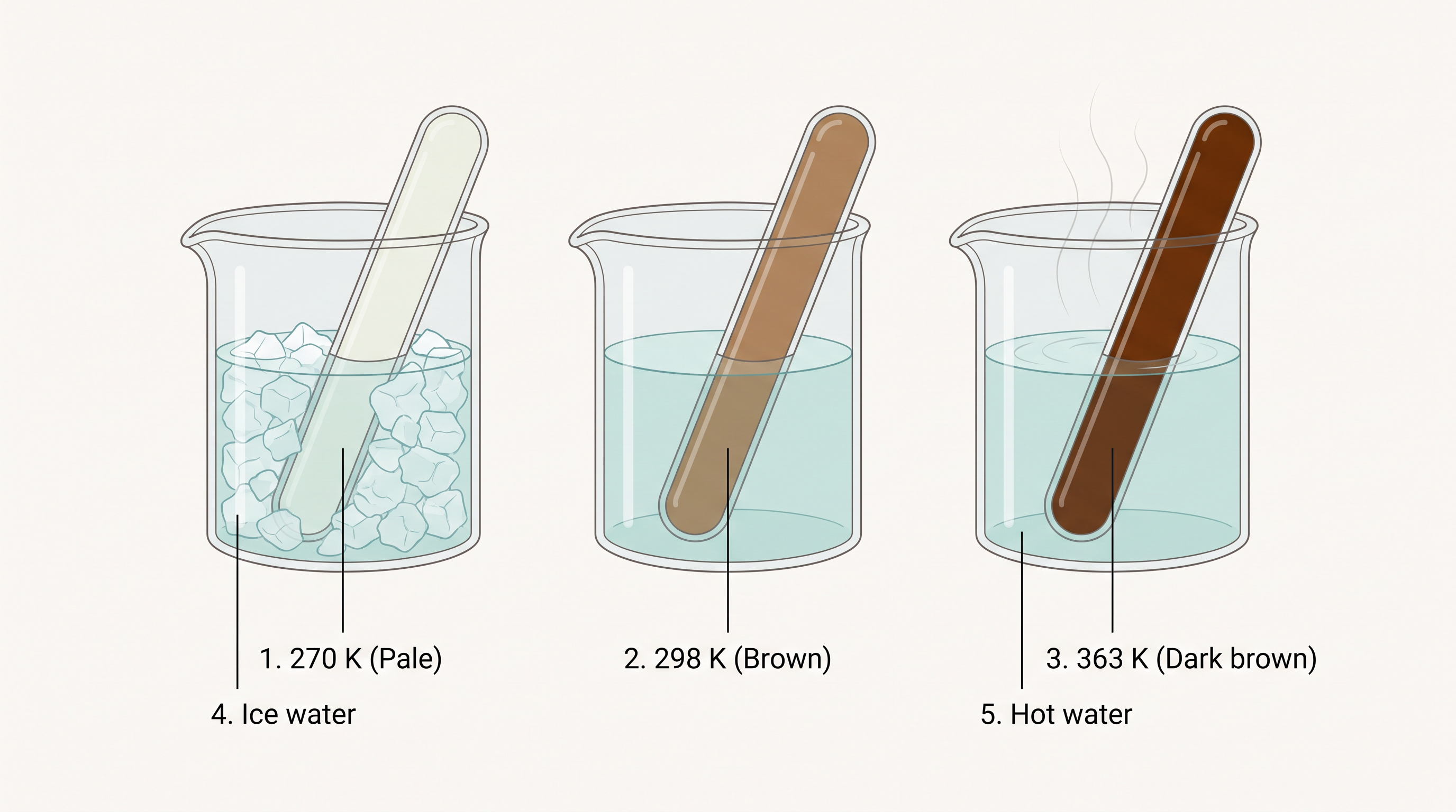
Fig. 6.9 – Effect of temperature on the NO₂ / N₂O₄ equilibrium.
The effect of temperature can also be seen in an endothermic reaction:
\[\mathrm{[\text{Co}(H_2O)_6]^{3+}}\text{(aq)} + 4\mathrm{Cl^{-}}\text{(aq)} \rightleftharpoons \mathrm{[\text{CoCl}_4]^{2-}}\text{(aq)} + 6\mathrm{H_2O}\text{(l)}\] \[\text{pink} \qquad \text{colourless} \qquad \text{blue}\]
At room temperature, the equilibrium mixture is blue due to \(\mathrm{[\text{CoCl}_4]^{2-}}\). When cooled in a freezing mixture, the colour of the mixture turns pink due to \(\mathrm{[\text{Co}(H_2O)_6]^{3+}}\) — cooling an endothermic reaction pushes it backward, exactly the opposite of the \(\mathrm{NO_2}\) case.
6.8.5 Effect of a Catalyst
A catalyst increases the rate of a chemical reaction by making available a new, low-energy pathway for the conversion of reactants to products. Crucially, it increases the rate of the forward and reverse reactions alike, because both pass through the same transition state — and so it does not affect equilibrium at all.
Here is the reasoning in full. A catalyst lowers the activation energy for the forward and reverse reactions by exactly the same amount. Both directions therefore speed up by the same factor, and their ratio — which is what determines the equilibrium position — is unchanged. A catalyst does not affect the equilibrium composition of a reaction mixture. It does not appear in the balanced chemical equation, and it does not appear in the equilibrium constant expression. What a catalyst does do is get the system to equilibrium faster.
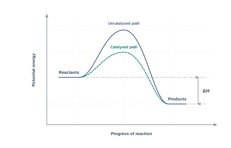
Fig. 6.10a – Effect of a catalyst on activation energy.
Let us apply this to ammonia formation from dinitrogen and dihydrogen. The reaction is highly exothermic and proceeds with a decrease in the total number of moles of gas formed compared to the reactants. Its equilibrium constant decreases with increase in temperature. At low temperature the rate decreases and the system takes a very long time to reach equilibrium; at high temperature the rate is satisfactory but the yield is poor. This is the classic industrial dilemma: good yield or good speed, but not both.
The German chemist Fritz Haber discovered that a catalyst consisting of iron catalyses the reaction to occur at a satisfactory rate at temperatures where the equilibrium concentration of \(\mathrm{NH_3}\) is reasonably favourable. And since the number of moles of gas formed in the reaction is less than that of the reactants, the yield of \(\mathrm{NH_3}\) can be improved by increasing the pressure — the pressure effect of Section 6.8.2, put to work.
Optimum conditions of temperature and pressure for the synthesis of \(\mathrm{NH_3}\) using a catalyst are around 500 °C and 200 atm.
Flowchart
FC 6.4 – Optimising the Haber process: exothermic reaction → low T favours yield but gives poor rate → raise T for rate, but yield falls → add iron catalyst to gain rate at moderate T (~500 °C) → forward reaction has fewer gas moles → raise pressure (~200 atm) to push yield back up → remove NH₃ by liquefaction to keep Qc < Kc → recycle unreacted N₂ and H₂.
A similar compromise appears in the manufacture of sulphuric acid by the contact process:
\[2\mathrm{SO_2}\text{(g)} + \mathrm{O_2}\text{(g)} \rightleftharpoons 2\mathrm{SO_3}\text{(g)}; \qquad K_c = 1.7 \times 10^{26}\]
Although this enormous value of \(K\) suggests the reaction should go essentially to completion, in practice the oxidation of \(\mathrm{SO_2}\) to \(\mathrm{SO_3}\) is very slow. A catalyst — platinum, or divanadium penta-oxide (\(\mathrm{V_2O_5}\)) — is therefore used to increase the rate of the reaction. This is a perfect demonstration that a large \(K\) tells you nothing about speed.
Note: If a reaction has an exceedingly small \(K\), a catalyst would be of little help. The catalyst can only get you to equilibrium faster; it cannot move the equilibrium to a place where the products are abundant. Speeding up the journey does not change the destination.
| Change made | Does the position of equilibrium shift? | Does the value of K change? | Reason |
|---|---|---|---|
| Add/remove a reactant or product | Yes | No | \(Q\) moves away from \(K\); the system shifts to restore \(Q = K\) |
| Change pressure (by changing volume), \(\Delta n \neq 0\) | Yes | No | Partial pressures change, so \(Q \neq K\); system moves toward fewer/more gas moles |
| Add an inert gas at constant volume | No | No | Partial pressures of reacting species are unchanged, so \(Q\) still equals \(K\) |
| Change temperature | Yes | Yes | \(K\) itself is temperature-dependent |
| Add a catalyst | No | No | Forward and reverse rates increase equally; only the time to reach equilibrium falls |
6.9 Ionic Equilibrium in Solution
Everything we have learned so far — the equilibrium constant, the reaction quotient, Le Chatelier’s principle — applies just as well to reactions that take place among ions in solution. In fact, you have already met one such equilibrium. When we studied the effect of concentration change, we used the reaction:
\[\mathrm{Fe^{3+}}\text{(aq)} + \mathrm{SCN^{-}}\text{(aq)} \rightleftharpoons \mathrm{[\text{Fe(SCN)}]^{2+}}\text{(aq)}\]
Every species here is an ion. There are countless equilibria of this kind, and the rest of this chapter is devoted to them.
Why some solutions conduct electricity
Begin with a simple observation. An aqueous solution of sugar does not conduct electricity. But add common salt (sodium chloride) to water, and the solution does conduct. Moreover, the conductance increases as the concentration of common salt increases — more dissolved salt, better conduction.
What is the difference? A sugar molecule stays whole in water; salt breaks apart into charged particles. Electric current in a solution is carried by moving ions, so a solution can conduct only if it contains free ions.
Michael Faraday classified substances into two categories on exactly this basis:
Substances that conduct electricity in their aqueous solutions are called electrolytes.
Substances that do not conduct are called non-electrolytes.
Strong and weak electrolytes
Faraday went further and divided electrolytes into two kinds, based on how completely they break into ions:
Strong electrolytes are ionized almost completely on dissolution in water.
Weak electrolytes are only partially dissociated.
Compare two familiar solutions. An aqueous solution of sodium chloride is comprised entirely of sodium ions and chloride ions — nothing is left whole. But a solution of acetic acid mainly contains unionized acetic acid molecules, with only some acetate ions and hydronium ions. The numbers make the contrast sharp: sodium chloride shows almost 100% ionization, while acetic acid — a weak electrolyte — shows less than 5% ionization.
| Feature | Strong electrolyte | Weak electrolyte |
|---|---|---|
| Extent of ionization in water | Almost complete (~100%) | Partial (e.g. less than 5% for acetic acid) |
| Species present in solution | Almost entirely ions | Mainly unionized molecules, plus some ions |
| Equilibrium between ions and molecules? | Essentially none — dissociation is complete | Yes — a genuine equilibrium exists |
| Conductivity of solution | High | Low |
| Example | Sodium chloride, \(\mathrm{NaCl}\) | Acetic acid, \(\mathrm{CH_3COOH}\) |
This last row of the table is where equilibrium enters the story. In a weak electrolyte, an equilibrium is established between the ions and the unionized molecules — some molecules are constantly breaking into ions while ions are constantly recombining into molecules, at equal rates. This type of equilibrium, involving ions in aqueous solution, is called ionic equilibrium.
Acids, bases and salts all come under the category of electrolytes, and each may act as either a strong or a weak electrolyte — which is precisely why we must study them next.
6.10 Acids, Bases and Salts
Acids, bases and salts are everywhere in nature — and inside you. Hydrochloric acid, present in gastric juice, is secreted by the lining of your stomach in a significant amount of 1.2–1.5 L per day, and is essential for digestive processes. Acetic acid is the main constituent of vinegar. Lemon and orange juices contain citric and ascorbic acids, and tartaric acid is found in tamarind paste.
Because most acids taste sour, the word “acid” itself carries the memory of that taste.
Acids turn blue litmus paper red and liberate dihydrogen on reacting with some metals. Bases behave oppositely: they turn red litmus paper blue, taste bitter, and feel soapy. A common example of a base is washing soda, used for washing purposes.
When acids and bases are mixed in the right proportion, they react with each other to give salts. Some commonly known examples of salts are sodium chloride, barium sulphate and sodium nitrate. Sodium chloride (common salt) is an important component of our diet, and is formed by the reaction between hydrochloric acid and sodium hydroxide.
How water pulls a salt apart
Solid sodium chloride exists as a cluster of positively charged sodium ions and negatively charged chloride ions, held together by electrostatic interactions between the oppositely charged species, as shown in Fig. 6.11. So why does water break this tight grip apart?
The answer lies in the dielectric constant of the solvent — a measure of how much a medium weakens the electrical force between two charges. The electrostatic force between two charges is inversely proportional to the dielectric constant of the medium. Water, a universal solvent, has a very high dielectric constant of 80. So when sodium chloride is dissolved in water, the electrostatic interactions holding \(\mathrm{Na^+}\) and \(\mathrm{Cl^-}\) together are reduced by a factor of 80. That is enough to let the ions move freely in solution. On top of this, the ions are kept well separated because they are hydrated — surrounded and stabilised by polar water molecules.
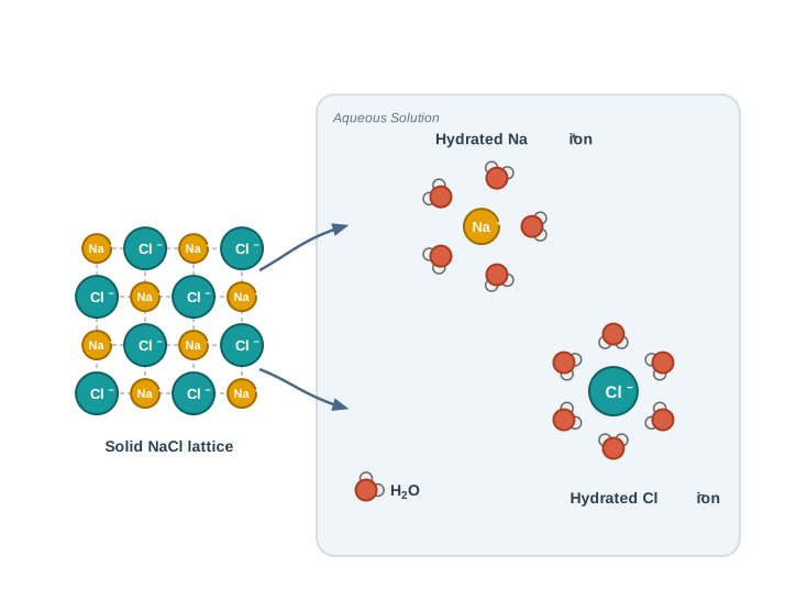
Fig. 6.11 – Dissolution of sodium chloride in water.
Ionization versus dissociation
Compare the ionization of hydrochloric acid with that of acetic acid in water. Though both are polar covalent molecules, the former is completely ionized into its constituent ions, while the latter is only partially ionized (< 5%). The extent to which ionization occurs depends on the strength of the bond and the extent of solvation of the ions produced.
The terms dissociation and ionization have historically carried different meanings. Dissociation refers to the separation, in water, of ions that already exist as such in the solid state of the solute — as in sodium chloride, where the ions were there all along. Ionization refers to a process in which a neutral molecule splits into charged ions in solution — as in acetic acid, where no ions existed before dissolving. In this chapter, we shall not distinguish between the two and will use the terms interchangeably.
6.10.1 Arrhenius Concept of Acids and Bases
The first modern definition came from Svante Arrhenius.
The ionization of an acid HX(aq) can be represented as:
\[\mathrm{HX}\text{(aq)} \rightarrow \mathrm{H^+}\text{(aq)} + \mathrm{X^-}\text{(aq)}\]
or, showing water’s role explicitly:
\[\mathrm{HX}\text{(aq)} + \mathrm{H_2O}\text{(l)} \rightarrow \mathrm{H_3O^+}\text{(aq)} + \mathrm{X^-}\text{(aq)}\]
Why the second form? Because a bare proton, \(\mathrm{H^+}\), is extremely reactive and cannot exist freely in aqueous solution. It immediately bonds to the oxygen atom of a solvent water molecule to give the trigonal pyramidal hydronium ion, \(\mathrm{H_3O^+}\), that is, \([\mathrm{H(H_2O)}]^+\). In this chapter we shall use \(\mathrm{H^+}\)(aq) and \(\mathrm{H_3O^+}\)(aq) interchangeably — both mean the same thing: a hydrated proton.
Hydronium and Hydroxyl Ions
A hydrogen ion by itself is a bare proton with a very small size (radius about \(10^{-15}\ \text{m}\)) and an intense electric field. Because of this, it binds itself to a water molecule at one of the two available lone pairs on oxygen, giving \(\mathrm{H_3O^+}\). This species has actually been detected in many compounds — for example \(\mathrm{H_3O^+Cl^-}\) — in the solid state.
In aqueous solution the hydronium ion is further hydrated, giving species such as \(\mathrm{H_5O_2^{+}}\), \(\mathrm{H_7O_3^{+}}\) and \(\mathrm{H_9O_4^{+}}\). Similarly, the hydroxyl ion is hydrated to give several ionic species like \(\mathrm{H_3O_2^{-}}\), \(\mathrm{H_5O_3^{-}}\) and \(\mathrm{H_7O_4^{-}}\).
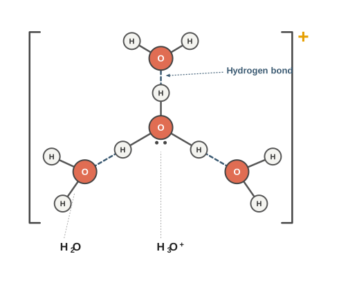
Fig. 6.12b – Structure of the H₉O₄⁺ ion.
Similarly, a base molecule MOH ionizes in aqueous solution:
\[\mathrm{MOH}\text{(aq)} \rightarrow \mathrm{M^+}\text{(aq)} + \mathrm{OH^-}\text{(aq)}\]
The hydroxyl ion also exists in hydrated form in aqueous solution.
The Arrhenius concept, however, has real limitations. It applies only to aqueous solutions, and it cannot account for the basicity of substances like ammonia, which possess no hydroxyl group at all. Something more general was needed.
6.10.2 The Brönsted-Lowry Acids and Bases
The Danish chemist Johannes Brönsted and the English chemist Thomas M. Lowry independently gave a more general definition of acids and bases, freeing the idea from any dependence on water.
Consider the dissolution of \(\mathrm{NH_3}\) in \(\mathrm{H_2O}\):
\[\mathrm{NH_3}\text{(aq)} + \mathrm{H_2O}\text{(l)} \rightleftharpoons \mathrm{NH_4^{+}}\text{(aq)} + \mathrm{OH^-}\text{(aq)}\]
\[\text{base} \qquad \text{acid} \qquad \text{conjugate acid} \qquad \text{conjugate base}\]
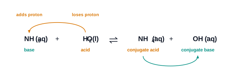
Fig. 6.13c – Proton transfer between ammonia and water.
The basic solution here is formed due to the presence of hydroxyl ions. Notice how the roles are assigned: the water molecule acts as proton donor and the ammonia molecule acts as proton acceptor — so they are the Lowry-Brönsted acid and base respectively. Ammonia is a base without possessing a single hydroxyl group, which is exactly the gap Arrhenius could not fill.
Now look at the reverse reaction. Here \(\mathrm{H^+}\) is transferred from \(\mathrm{NH_4^{+}}\) to \(\mathrm{OH^-}\). In this case, \(\mathrm{NH_4^{+}}\) acts as a Brönsted acid while \(\mathrm{OH^-}\) acts as a Brönsted base. So every Brönsted-Lowry reaction has acids and bases on both sides.
An acid-base pair that differs only by one proton is called a conjugate acid-base pair. In the reaction above, \(\mathrm{OH^-}\) is the conjugate base of the acid \(\mathrm{H_2O}\), and \(\mathrm{NH_4^{+}}\) is the conjugate acid of the base \(\mathrm{NH_3}\).
Two rules follow, and both are exam-critical. If a Brönsted acid is a strong acid, then its conjugate base is a weak base, and vice-versa. Also, a conjugate acid always has one extra proton and each conjugate base has one less proton than its partner.
Consider the ionization of hydrochloric acid in water. HCl(aq) acts as an acid by donating a proton to the \(\mathrm{H_2O}\) molecule, which acts as a base:
\[\mathrm{HCl}\text{(aq)} + \mathrm{H_2O}\text{(l)} \rightleftharpoons \mathrm{H_3O^+}\text{(aq)} + \mathrm{Cl^-}\text{(aq)}\]
\[\text{acid} \qquad \text{base} \qquad \text{conjugate acid} \qquad \text{conjugate base}\]

Fig. 6.14d – Proton transfer between hydrochloric acid and water.
Here water acts as a base, because it accepts the proton. The species \(\mathrm{H_3O^+}\) is produced when water accepts a proton from HCl. Therefore \(\mathrm{Cl^-}\) is the conjugate base of HCl, and HCl is the conjugate acid of the base \(\mathrm{Cl^-}\). Similarly, \(\mathrm{H_2O}\) is the conjugate base of the acid \(\mathrm{H_3O^+}\), and \(\mathrm{H_3O^+}\) is the conjugate acid of the base \(\mathrm{H_2O}\).
Now compare the two examples and something interesting emerges: the dual role of water. In the reaction with HCl, water acts as a base (accepting a proton). In the reaction with ammonia, water acts as an acid (donating a proton). Water can do both — a property that will become central when we study the ionization of water itself.
6.10.3 Lewis Acids and Bases
There is a still broader definition. G.N. Lewis, in 1923, defined an acid as a species which accepts an electron pair and a base as one which donates an electron pair.
As far as bases are concerned, there is not much difference between the Brönsted-Lowry and Lewis concepts — the base provides a lone pair in both cases. The real gain is on the acid side. In the Lewis concept, many acids do not have a proton at all. That is a genuine extension: neither Arrhenius nor Brönsted-Lowry could call a proton-free species an acid.
A typical example is the reaction of the electron-deficient species \(\mathrm{BF_3}\) with \(\mathrm{NH_3}\). \(\mathrm{BF_3}\) does not have a proton, but it still acts as an acid — it reacts with \(\mathrm{NH_3}\) by accepting its lone pair of electrons:
\[\mathrm{BF_3} + :\mathrm{NH_3} \rightarrow \mathrm{BF_3}!:!\mathrm{NH_3}\]

Fig. 6.15e – Lewis acid-base reaction between BF₃ and NH₃.
Electron-deficient species like \(\mathrm{AlCl_3}\), \(\mathrm{Co^{3+}}\), \(\mathrm{Mg^{2+}}\), etc. can act as Lewis acids, while species like \(\mathrm{H_2O}\), \(\mathrm{NH_3}\), \(\mathrm{OH^-}\), etc., which can donate a pair of electrons, can act as Lewis bases.
|Feature|Arrhenius|Brönsted-Lowry|Lewis|
|-|-|-|-|
|Acid is…|a substance giving \(\mathrm{H^+}\)(aq) in water|a proton donor|an electron-pair acceptor|
|Base is…|a substance giving \(\mathrm{OH^-}\)(aq) in water|a proton acceptor|an electron-pair donor|
|Needs water as solvent?|Yes|No|No|
|Must the acid contain H?|Yes|Yes|No|
|Can explain \(\mathrm{NH_3}\) as a base?|No (no OH group)|Yes|Yes|
|Can explain \(\mathrm{BF_3}\) as an acid?|No|No (no proton)|Yes|
|Example acid|HCl|HCl, \(\mathrm{NH_4^{+}}\)|\(\mathrm{BF_3}\), \(\mathrm{AlCl_3}\), \(\mathrm{H^+}\)|
Notice the pattern: each concept is broader than the last, and each contains the one before it. Every Arrhenius acid is a Brönsted acid, and every Brönsted acid is a Lewis acid — but not the other way round.
6.11 Ionization of Acids and Bases
The Arrhenius concept of acids and bases becomes especially useful when we study ionization, because most ionizations in chemical and biological systems occur in aqueous medium.
Some acids are called strong because they are almost completely dissociated into their constituent ions in aqueous medium, thereby acting as excellent proton (\(\mathrm{H^+}\)) donors. The strong acids are perchloric acid (\(\mathrm{HClO_4}\)), hydrochloric acid (\(\mathrm{HCl}\)), hydrobromic acid (\(\mathrm{HBr}\)), hydroiodic acid (\(\mathrm{HI}\)), nitric acid (\(\mathrm{HNO_3}\)) and sulphuric acid (\(\mathrm{H_2SO_4}\)).
Similarly, strong bases like lithium hydroxide (\(\mathrm{LiOH}\)), sodium hydroxide (\(\mathrm{NaOH}\)), potassium hydroxide (\(\mathrm{KOH}\)), caesium hydroxide (\(\mathrm{CsOH}\)) and barium hydroxide (\(\mathrm{Ba(OH)_2}\)) are almost completely dissociated into ions in aqueous medium, giving hydroxyl ions, \(\mathrm{OH^-}\). According to the Arrhenius concept, these are strong acids and bases because they are able to completely dissociate and produce \(\mathrm{H_3O^+}\) and \(\mathrm{OH^-}\) ions respectively in the medium.
The strength of an acid or base can also be judged using the Brönsted-Lowry concept, where a strong acid means a good proton donor and a strong base implies a good proton acceptor.
Which side does a dissociation equilibrium favour?
Consider the acid-base dissociation equilibrium of a weak acid HA:
\[\mathrm{HA}\text{(aq)} + \mathrm{H_2O}\text{(l)} \rightleftharpoons \mathrm{H_3O^+}\text{(aq)} + \mathrm{A^-}\text{(aq)}\]
\[\text{acid} \qquad \text{base} \qquad \text{conjugate acid} \qquad \text{conjugate base}\]
We know this equilibrium is dynamic, with protons being transferred in both directions. But if it is dynamic, which direction is favoured over time? What is the driving force?
To answer, compare the strengths of the two acids present in the equilibrium: HA and \(\mathrm{H_3O^+}\). Whichever of them is the better proton donor is the stronger acid, and the equilibrium shifts in the direction of the weaker acid. Say HA is a stronger acid than \(\mathrm{H_3O^+}\). Then HA will donate protons and \(\mathrm{H_3O^+}\) will not, so the solution will mainly contain \(\mathrm{A^-}\) and \(\mathrm{H_3O^+}\) ions. The equilibrium moves in the direction of formation of the weaker acid and weaker base — because the stronger acid donates a proton to the stronger base.
Strong acids have weak conjugate bases
An important consequence follows. As a strong acid dissociates completely in water, the base formed from it must be very weak — because it has almost no tendency to take the proton back. So: strong acids have very weak conjugate bases.
Strong acids like perchloric acid (\(\mathrm{HClO_4}\)), hydrochloric acid (\(\mathrm{HCl}\)), hydrobromic acid (\(\mathrm{HBr}\)), hydroiodic acid (\(\mathrm{HI}\)), nitric acid (\(\mathrm{HNO_3}\)) and sulphuric acid (\(\mathrm{H_2SO_4}\)) will give conjugate base ions \(\mathrm{ClO_4^{-}}\), \(\mathrm{Cl^-}\), \(\mathrm{Br^-}\), \(\mathrm{I^-}\), \(\mathrm{NO_3^{-}}\) and \(\mathrm{HSO_4^{-}}\), which are much weaker bases than \(\mathrm{H_2O}\). Similarly, a very strong base gives a very weak conjugate acid.
The mirror statement is equally true. A weak acid like HA is only partially dissociated in aqueous medium, so the solution mainly contains undissociated HA molecules. Typical weak acids are nitrous acid (\(\mathrm{HNO_2}\)), hydrofluoric acid (\(\mathrm{HF}\)) and acetic acid (\(\mathrm{CH_3COOH}\)). And weak acids have very strong conjugate bases. For example, \(\mathrm{NH_2^{-}}\), \(\mathrm{O^{2-}}\) and \(\mathrm{H^-}\) are very good proton acceptors and thus much stronger bases than \(\mathrm{H_2O}\).
Indicators as weak acids
Certain water-soluble organic compounds like phenolphthalein and bromothymol blue behave as weak acids and exhibit different colours in their acid (HIn) and conjugate base (In⁻) forms:
\[\mathrm{HIn}\text{(aq)} + \mathrm{H_2O}\text{(l)} \rightleftharpoons \mathrm{H_3O^+}\text{(aq)} + \mathrm{In^-}\text{(aq)}\]
\[\text{acid indicator} \qquad \text{conjugate acid} \qquad \text{conjugate base}\]
\[\text{colour A} \qquad\qquad\qquad\qquad \text{colour B}\]
The chemistry here is simply Le Chatelier’s principle in disguise. Adding acid pushes the equilibrium left (colour A); adding base pulls it right (colour B). Such compounds are therefore useful as indicators in acid-base titrations, and for finding out the \(\mathrm{H^+}\) ion concentration.
6.11.1 The Ionization Constant of Water and its Ionic Product
Some substances, like water, are unique in their ability to act both as an acid and a base. We saw this in section 6.10.2. In the presence of an acid HA, water accepts a proton and acts as the base; in the presence of a base \(\mathrm{B^-}\), it donates a proton and acts as an acid.
What happens, then, in pure water, where there is nothing else present? Water must play both roles at once. One \(\mathrm{H_2O}\) molecule donates a proton and acts as an acid, while another \(\mathrm{H_2O}\) molecule accepts that proton and acts as a base. The following equilibrium exists:
\[\mathrm{H_2O}\text{(l)} + \mathrm{H_2O}\text{(l)} \rightleftharpoons \mathrm{H_3O^+}\text{(aq)} + \mathrm{OH^-}\text{(aq)}\]
\[\text{acid} \qquad \text{base} \qquad \text{conjugate acid} \qquad \text{conjugate base}\]
The dissociation constant is represented by:
\[K = \frac{[\mathrm{H_3O^+}][\mathrm{OH^-}]}{[\mathrm{H_2O}]} \qquad (6.26)\]
But the concentration of water is omitted from the denominator, because water is a pure liquid and its concentration remains constant — exactly the reasoning we used for pure solids and liquids in Section 6.5. Absorbing \([\mathrm{H_2O}]\) into the equilibrium constant gives a new constant, \(K_w\), called the ionic product of water:
\[K_w = [\mathrm{H^+}][\mathrm{OH^-}] \qquad (6.27)\]
The concentration of \(\mathrm{H^+}\) has been found experimentally as \(1.0 \times 10^{-7}\ \text{M}\) at 298 K. And since the dissociation of water produces equal numbers of \(\mathrm{H^+}\) and \(\mathrm{OH^-}\) ions, the concentration of hydroxyl ions must be the same: \([\mathrm{OH^-}] = [\mathrm{H^+}] = 1.0 \times 10^{-7}\ \text{M}\). Thus, the value of \(K_w\) at 298 K is:
\[K_w = [\mathrm{H_3O^+}][\mathrm{OH^-}] = (1 \times 10^{-7})^2 = 1 \times 10^{-14}\ \text{M}^2 \qquad (6.28)\]
How little of water is actually ionized
It is worth pausing to see how tiny this dissociation really is. The density of pure water is 1000 g/L and its molar mass is 18.0 g/mol. From this, the molarity of pure water is:
\[[\mathrm{H_2O}] = (1000\ \text{g/L})(1\ \text{mol}/18.0\ \text{g}) = 55.55\ \text{M}\]
Therefore, the ratio of dissociated water to undissociated water is:
\[\frac{10^{-7}}{55.55} = 1.8 \times 10^{-9}\ \text{, or about 2 in } 10^{9}\]
Only about two water molecules in a billion are ionized at any instant. The equilibrium lies overwhelmingly toward undissociated water — which is why pure water is such a poor conductor of electricity.
We can now distinguish acidic, neutral and basic aqueous solutions by the relative values of the \(\mathrm{H_3O^+}\) and \(\mathrm{OH^-}\) concentrations:
Acidic: \([\mathrm{H_3O^+}] > [\mathrm{OH^-}]\)
Neutral: \([\mathrm{H_3O^+}] = [\mathrm{OH^-}]\)
Basic: \([\mathrm{H_3O^+}] < [\mathrm{OH^-}]\)
6.11.2 The pH Scale
Hydronium ion concentrations are awkward numbers — \(10^{-7}\), \(10^{-3}\), \(10^{-11}\). They are more conveniently expressed on a logarithmic scale known as the pH scale. This is exactly why a logarithm appears here: it turns an unwieldy range spanning fifteen powers of ten into a tidy scale running roughly from 0 to 14.
In dilute solutions (< 0.01 M), the activity of the hydrogen ion is equal in magnitude to the molarity, represented by \([\mathrm{H^+}]\). Activity has no units and is defined as:
\[a_{\mathrm{H^+}} = [\mathrm{H^+}]\,/\,\text{mol L}^{-1}\]
From the definition of pH, we can therefore write:
\[\mathrm{pH} = -\log a_{\mathrm{H^+}} = -\log{[\mathrm{H^+}]\,/\,\text{mol L}^{-1}}\]
Some quick applications. An acidic solution of HCl (\(10^{-2}\ \text{M}\)) will have a pH of 2. A basic solution of NaOH having \([\mathrm{OH^-}] = 10^{-4}\ \text{M}\) and \([\mathrm{H_3O^+}] = 10^{-10}\ \text{M}\) will have a pH of 10. At 25 °C, pure water has \([\mathrm{H^+}] = 10^{-7}\ \text{M}\), so the pH of pure water is:
\[\mathrm{pH} = -\log(10^{-7}) = 7\]
Acidic solutions possess a concentration of hydrogen ions \([\mathrm{H^+}] > 10^{-7}\ \text{M}\), while basic solutions possess \([\mathrm{H^+}] < 10^{-7}\ \text{M}\). Because pH is a negative logarithm, a higher \([\mathrm{H^+}]\) gives a lower pH — the scale runs backwards from what you might expect. Summarising:
Acidic solution has pH < 7
Basic solution has pH > 7
Neutral solution has pH = 7
Relating pH and pOH
Now return to equation (6.28) at 298 K:
\[K_w = [\mathrm{H_3O^+}][\mathrm{OH^-}] = 10^{-14}\]
Take the negative logarithm of both sides:
\[-\log K_w = -\log{[\mathrm{H_3O^+}][\mathrm{OH^-}]}\]
\[= -\log[\mathrm{H_3O^+}] - \log[\mathrm{OH^-}]\]
\[= -\log 10^{-14}\]
(using the rule that the logarithm of a product is the sum of the logarithms). This gives the extremely useful relation:
\[\mathrm{p}K_w = \mathrm{pH} + \mathrm{pOH} = 14 \qquad (6.29)\]
Note that although \(K_w\) may change with temperature, the variations in pH with temperature are so small that we often ignore them.
\(\mathrm{p}K_w\) is a very important quantity for aqueous solutions, and it controls the relative concentrations of hydrogen and hydroxyl ions, as their product is a constant. It should also be noted that because the pH scale is logarithmic, a change in pH by just one unit means a change in \([\mathrm{H^+}]\) by a factor of 10. Similarly, when \([\mathrm{H^+}]\) changes by a factor of 100, the value of pH changes by 2 units. This is why the small changes in pH with temperature can be ignored — they correspond to almost no change in \([\mathrm{H^+}]\).
Measuring pH
Measurement of pH is very important, since its value must be known when dealing with biological and cosmetic applications. The pH of a solution can be found roughly with the help of pH paper, which shows a different colour in solutions of different pH. Modern pH paper is available with four strips on it; the different strips show different colours (Fig. 6.16) at the same pH, and comparing the set gives a better reading. The pH in the range of 1–14 can be determined with an accuracy of about \(\pm 0.5\) using pH paper.
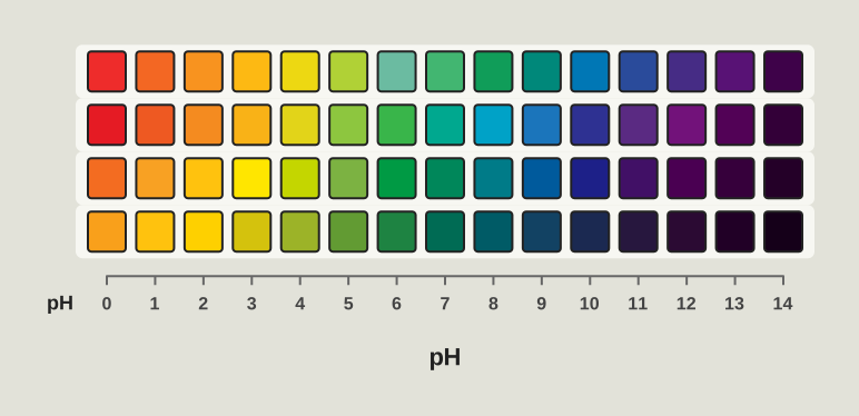
Fig. 6.16 – A four-strip pH paper colour chart.
For greater accuracy, pH meters are used. A pH meter is a device that measures the pH-dependent electrical potential of the test solution to within 0.001 precision. pH meters the size of a writing pen are now available in the market.
The pH values of some very common substances are given in Table 6.5.
Table 6.5 The pH of Some Common Substances
|Name of the Fluid|pH|Name of the Fluid|pH|
|-|-|-|-|
|Saturated solution of NaOH|~15|Black Coffee|5.0|
|0.1 M NaOH solution|13|Tomato juice|~4.2|
|Lime water|10.5|Soft drinks and vinegar|~3.0|
|Milk of magnesia|10|Lemon juice|~2.2|
|Egg white, sea water|7.8|Gastric juice|~1.2|
|Human blood|7.4|1 M HCl solution|~0|
|Milk|6.8|Concentrated HCl|~ –1.0|
|Human Saliva|6.4|||
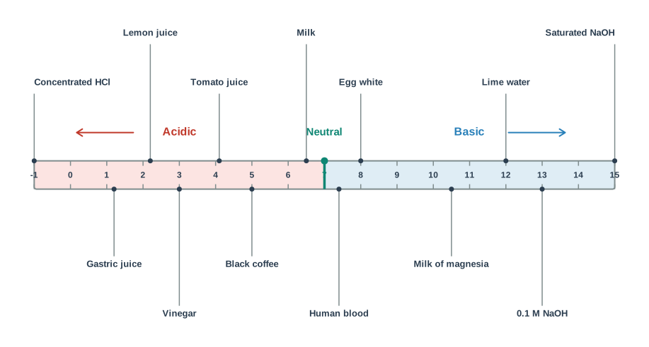
Fig. 6.17a – The pH scale with common substances.
6.11.3 Ionization Constants of Weak Acids
Consider a weak acid HX that is partially ionized in aqueous solution. The equilibrium can be expressed by:
\[\mathrm{HX}\text{(aq)} + \mathrm{H_2O}\text{(l)} \rightleftharpoons \mathrm{H_3O^+}\text{(aq)} + \mathrm{X^-}\text{(aq)}\]
Let us track the concentrations. Let \(c\) = initial concentration of the undissociated acid HX at time \(t = 0\), and \(\alpha\) = the degree of ionization, that is, the fraction of HX that is ionized into ions.
Initial concentration (M): \(c\), \(0\), \(0\)
Change (M): \(-c\alpha\), \(+c\alpha\), \(+c\alpha\)
Equilibrium concentration (M): \(c - c\alpha\), \(c\alpha\), \(c\alpha\)
Using these notations, we derive the equilibrium constant for this acid-dissociation equilibrium:
\[K_a = \frac{c^2\alpha^2}{c(1-\alpha)} = \frac{c\alpha^2}{1-\alpha}\]
\(K_a\) is called the dissociation or ionization constant of the acid HX. It can be represented alternatively in terms of molar concentration:
\[K_a = \frac{[\mathrm{H^+}][\mathrm{X^-}]}{[\mathrm{HX}]} \qquad (6.30)\]
Why does a bigger \(K_a\) mean a stronger acid? Because \(K_a\) has the ions in the numerator and the undissociated acid in the denominator. A large \(K_a\) therefore means the equilibrium lies far to the ionized side — the acid gives up its proton readily. That is exactly what “strong” means.
The values of the ionization constants of some selected weak acids are given in Table 6.6.
Table 6.6 The Ionization Constants of Some Selected Weak Acids (at 298 K)
|Acid|Ionization Constant, \(K_a\)|
|-|-|
|Hydrofluoric Acid (HF)|\(3.5 \times 10^{-4}\)|
|Nitrous Acid (\(\mathrm{HNO_2}\))|\(4.5 \times 10^{-4}\)|
|Formic Acid (HCOOH)|\(1.8 \times 10^{-4}\)|
|Niacin (\(\mathrm{C_5H_4NCOOH}\))|\(1.5 \times 10^{-5}\)|
|Acetic Acid (\(\mathrm{CH_3COOH}\))|\(1.74 \times 10^{-5}\)|
|Benzoic Acid (\(\mathrm{C_6H_5COOH}\))|\(6.5 \times 10^{-5}\)|
|Hypochlorous Acid (HClO)|\(3.0 \times 10^{-8}\)|
|Hydrocyanic Acid (HCN)|\(4.9 \times 10^{-10}\)|
|Phenol (\(\mathrm{C_6H_5OH}\))|\(1.3 \times 10^{-10}\)|
The pH scale for the hydrogen ion concentration has proved so useful that, besides \(\mathrm{p}K_w\), it has been extended to other species and quantities. Thus we have:
\[\mathrm{p}K_a = -\log(K_a) \qquad (6.31)\]
A smaller \(\mathrm{p}K_a\) means a stronger acid — the minus sign flips the direction, just as it does for pH.
Knowing the ionization constant \(K_a\) of an acid and its initial concentration \(c\), it is possible to calculate the equilibrium concentration of all species, the degree of ionization of the acid, and the pH of the solution.
A step-wise approach for weak-electrolyte pH
A general step-wise approach can be adopted to evaluate the pH of a weak electrolyte:
Step 1. The species present before dissociation are identified as Brönsted-Lowry acids/bases.
Step 2. Balanced equations for all possible reactions are written, i.e., with a species acting both as acid and as base.
Step 3. The reaction with the higher \(K_a\) is identified as the primary reaction, whilst the other is a subsidiary reaction.
Step 4. Enlist in a tabular form the following values for each of the species in the primary reaction: (a) initial concentration, \(c\); (b) change in concentration on proceeding to equilibrium in terms of \(\alpha\), the degree of ionization; (c) equilibrium concentration.
Step 5. Substitute equilibrium concentrations into the equilibrium constant equation for the principal reaction and solve for \(\alpha\).
Step 6. Calculate the concentration of species in the principal reaction.
Step 7. Calculate \(\mathrm{pH} = -\log[\mathrm{H_3O^+}]\).
Flowchart
FC 6.5 – Finding the pH of a weak acid: identify all Brönsted acids/bases present → write every possible balanced equilibrium → compare Ka values → pick the larger-Ka reaction as the principal one (the other is subsidiary) → build the initial/change/equilibrium table in terms of α → substitute into Ka and solve for α → compute [H₃O⁺] = cα → pH = –log[H₃O⁺].
The above methodology is elucidated in the following examples.
Percent dissociation
Alternatively, “percent dissociation” is another useful method for measuring the strength of a weak acid, and is given as:
\[\text{Percent dissociation} = \frac{[\mathrm{HA}]_{\text{dissociated}}}{[\mathrm{HA}]_{\text{initial}}} \times 100\% \qquad (6.32)\]
6.11.4 Ionization of Weak Bases
The ionization of a base MOH can be represented by the equation:
\[\mathrm{MOH}\text{(aq)} \rightleftharpoons \mathrm{M^+}\text{(aq)} + \mathrm{OH^-}\text{(aq)}\]
In a weak base there is only partial ionization of MOH into \(\mathrm{M^+}\) and \(\mathrm{OH^-}\) — the case is exactly parallel to acid-dissociation equilibrium. The equilibrium constant for base ionization is called the base ionization constant and is represented by \(K_b\). It can be expressed in terms of molar concentrations by:
\[K_b = \frac{[\mathrm{M^+}][\mathrm{OH^-}]}{[\mathrm{MOH}]} \qquad (6.33)\]
Alternatively, if \(c\) = initial concentration of base and \(\alpha\) = degree of ionization of the base (the extent to which the base ionizes), then when equilibrium is reached:
\[K_b = \frac{(c\alpha)^2}{c(1-\alpha)} = \frac{c\alpha^2}{(1-\alpha)}\]
Note how this mirrors the acid expression exactly. The values of the ionization constants of some selected weak bases are given in Table 6.7.
Table 6.7 The Values of the Ionization Constant of Some Weak Bases at 298 K
|Base|\(K_b\)|
|-|-|
|Dimethylamine, \(\mathrm{(CH_3)_2NH}\)|\(5.4 \times 10^{-4}\)|
|Triethylamine, \(\mathrm{(C_2H_5)_3N}\)|\(6.45 \times 10^{-5}\)|
|Ammonia, \(\mathrm{NH_3}\) or \(\mathrm{NH_4OH}\)|\(1.77 \times 10^{-5}\)|
|Quinine, (A plant product)|\(1.10 \times 10^{-6}\)|
|Pyridine, \(\mathrm{C_5H_5N}\)|\(1.77 \times 10^{-9}\)|
|Aniline, \(\mathrm{C_6H_5NH_2}\)|\(4.27 \times 10^{-10}\)|
|Urea, \(\mathrm{CO(NH_2)_2}\)|\(1.3 \times 10^{-14}\)|
Many organic compounds like amines are weak bases. Amines are derivatives of ammonia in which one or more hydrogen atoms are replaced by another group. For example, methylamine, codeine, quinine and nicotine all behave as very weak bases due to their very small \(K_b\). Ammonia produces \(\mathrm{OH^-}\) in aqueous solution:
\[\mathrm{NH_3}\text{(aq)} + \mathrm{H_2O}\text{(l)} \rightleftharpoons \mathrm{NH_4^{+}}\text{(aq)} + \mathrm{OH^-}\text{(aq)}\]
The pH scale for the hydrogen ion concentration has been extended to give:
\[\mathrm{p}K_b = -\log(K_b) \qquad (6.34)\]
6.11.5 Relation between \(K_a\) and \(K_b\)
As seen earlier, \(K_a\) and \(K_b\) represent the strength of an acid and a base respectively. In the case of a conjugate acid-base pair, the two are related in a beautifully simple way — so that if one is known, the other can be deduced immediately.
Consider the example of \(\mathrm{NH_4^{+}}\) and \(\mathrm{NH_3}\), which form a conjugate pair. Write both equilibria:
\[\mathrm{NH_4^{+}}\text{(aq)} + \mathrm{H_2O}\text{(l)} \rightleftharpoons \mathrm{H_3O^+}\text{(aq)} + \mathrm{NH_3}\text{(aq)}\]
\[K_a = \frac{[\mathrm{H_3O^+}][\mathrm{NH_3}]}{[\mathrm{NH_4^{+}}]} = 5.6 \times 10^{-10}\]
\[\mathrm{NH_3}\text{(aq)} + \mathrm{H_2O}\text{(l)} \rightleftharpoons \mathrm{NH_4^{+}}\text{(aq)} + \mathrm{OH^-}\text{(aq)}\]
\[K_b = \frac{[\mathrm{NH_4^{+}}][\mathrm{OH^-}]}{[\mathrm{NH_3}]} = 1.8 \times 10^{-5}\]
Now add the two equations. The \(\mathrm{NH_4^{+}}\) and \(\mathrm{NH_3}\) terms cancel on each side, leaving the net reaction:
\[\text{Net: } 2\,\mathrm{H_2O}\text{(l)} \rightleftharpoons \mathrm{H_3O^+}\text{(aq)} + \mathrm{OH^-}\text{(aq)}\]
\[K_w = [\mathrm{H_3O^+}][\mathrm{OH^-}] = 1.0 \times 10^{-14}\ \text{M}\]
Here \(K_a\) represents the strength of \(\mathrm{NH_4^{+}}\) as an acid and \(K_b\) represents the strength of \(\mathrm{NH_3}\) as a base.
It can be seen from the net reaction that the equilibrium constant is equal to the product of the equilibrium constants \(K_a\) and \(K_b\) for the reactions added. Thus:
\[K_a \times K_b = \left\{\frac{[\mathrm{H_3O^+}][\mathrm{NH_3}]}{[\mathrm{NH_4^{+}}]}\right\} \times \left\{\frac{[\mathrm{NH_4^{+}}][\mathrm{OH^-}]}{[\mathrm{NH_3}]}\right\}\]
\[= [\mathrm{H_3O^+}][\mathrm{OH^-}] = K_w\]
\[= (5.6 \times 10^{-10}) \times (1.8 \times 10^{-5}) = 1.0 \times 10^{-14}\ \text{M}\]
This can be extended into a general rule.
Similarly, in the case of a conjugate acid-base pair:
\[K_a \times K_b = K_w \qquad (6.36)\]
Knowing one, the other can be obtained. It should be noted that this relation is the quantitative form of the qualitative rule we met earlier: a strong acid will have a weak conjugate base and vice-versa. Since their product is fixed at \(K_w\), whenever \(K_a\) is large, \(K_b\) must be small.
Deriving the same result from the base side
Alternatively, the expression \(K_w = K_a \times K_b\) can also be obtained by considering the base-dissociation equilibrium reaction:
\[\mathrm{B}\text{(aq)} + \mathrm{H_2O}\text{(l)} \rightleftharpoons \mathrm{BH^+}\text{(aq)} + \mathrm{OH^-}\text{(aq)}\]
\[K_b = \frac{[\mathrm{BH^+}][\mathrm{OH^-}]}{[\mathrm{B}]}\]
(As the concentration of water remains constant, it has been omitted from the denominator and incorporated within the dissociation constant.) Now multiply and divide the above expression by \([\mathrm{H^+}]\):
\[K_b = \frac{[\mathrm{BH^+}][\mathrm{OH^-}][\mathrm{H^+}]}{[\mathrm{B}][\mathrm{H^+}]} = {[\mathrm{OH^-}][\mathrm{H^+}]}\left\{\frac{[\mathrm{BH^+}]}{[\mathrm{B}][\mathrm{H^+}]}\right\} = \frac{K_w}{K_a}\]
or
\[K_a \times K_b = K_w\]
It may be noted that if we take the negative logarithm of both sides of this equation, then the \(\mathrm{p}K\) values of the conjugate acid and base are related by:
\[\mathrm{p}K_a + \mathrm{p}K_b = \mathrm{p}K_w = 14 \quad (\text{at } 298\ \text{K})\]
6.11.6 Di- and Polybasic Acids and Di- and Polyacidic Bases
Some acids — like oxalic acid, sulphuric acid and phosphoric acid — have more than one ionizable proton per molecule. Such acids are known as polybasic or polyprotic acids.
They do not release all their protons at once. Instead they ionize in successive steps, one proton at a time, each step having its own equilibrium constant. The ionization reactions for a dibasic acid \(\mathrm{H_2X}\) are represented by:
\[\mathrm{H_2X}\text{(aq)} \rightleftharpoons \mathrm{H^+}\text{(aq)} + \mathrm{HX^-}\text{(aq)}\]
\[\mathrm{HX^-}\text{(aq)} \rightleftharpoons \mathrm{H^+}\text{(aq)} + \mathrm{X^{2-}}\text{(aq)}\]
And the corresponding equilibrium constants are:
\[K_{a_1} = \frac{[\mathrm{H^+}][\mathrm{HX^-}]}{[\mathrm{H_2X}]} \qquad\text{and}\qquad K_{a_2} = \frac{[\mathrm{H^+}][\mathrm{X^{2-}}]}{[\mathrm{HX^-}]}\]
Here \(K_{a_1}\) and \(K_{a_2}\) are called the first and second ionization constants respectively of the acid \(\mathrm{H_2X}\). Similarly, for tribasic acids like \(\mathrm{H_3PO_4}\) we have three ionization constants. The values for some common polyprotic acids are given in Table 6.8.
Table 6.8 The Ionization Constants of Some Common Polyprotic Acids (298 K)
|Acid|\(K_{a_1}\)|\(K_{a_2}\)|\(K_{a_3}\)|
|-|-|-|-|
|Oxalic Acid|\(5.9 \times 10^{-2}\)|\(6.4 \times 10^{-5}\)||
|Ascorbic Acid|\(7.4 \times 10^{-4}\)|\(1.6 \times 10^{-12}\)||
|Sulphurous Acid|\(1.7 \times 10^{-2}\)|\(6.4 \times 10^{-8}\)||
|Sulphuric Acid|Very large|\(1.2 \times 10^{-2}\)||
|Carbonic Acid|\(4.3 \times 10^{-7}\)|\(5.6 \times 10^{-11}\)||
|Citric Acid|\(7.4 \times 10^{-4}\)|\(1.7 \times 10^{-5}\)|\(4.0 \times 10^{-7}\)|
|Phosphoric Acid|\(7.5 \times 10^{-3}\)|\(6.2 \times 10^{-8}\)|\(4.2 \times 10^{-13}\)|
Look down any row of the table and one pattern is unmistakable: the higher-order ionization constants (\(K_{a_2}\), \(K_{a_3}\)) are always smaller than the lower-order one (\(K_{a_1}\)) — often by many powers of ten.
The reason is electrostatic. It is much more difficult to remove a positively charged proton from a negative ion than from a neutral molecule, because the negative charge holds the proton back. Compare removing a proton from the uncharged \(\mathrm{H_2CO_3}\) with removing one from the negatively charged \(\mathrm{HCO_3^{-}}\) — the second is far harder. Similarly, it is more difficult to remove a proton from a doubly charged \(\mathrm{HPO_4^{2-}}\) anion than from \(\mathrm{H_2PO_4^{-}}\). Each proton removed leaves behind a more negative species, which grips the next proton more tightly.
Polyprotic acid solutions contain a mixture of acids like \(\mathrm{H_2A}\), \(\mathrm{HA^-}\) and \(\mathrm{A^{2-}}\) in the case of a diprotic acid. Since \(\mathrm{H_2A}\) is the strongest of these, the primary reaction involves the dissociation of \(\mathrm{H_2A}\), and the \(\mathrm{H_3O^+}\) in the solution comes mainly from the first dissociation step. This is a great practical simplification: for most calculations, you can ignore the later steps entirely.
6.11.7 Factors Affecting Acid Strength
Having discussed the strengths of acids and bases quantitatively, we can now calculate the pH of a given acid solution. But the curiosity remains: why should some acids be stronger than others? What factors make them stronger?
The answer is a complex phenomenon, but broadly speaking, the extent of dissociation of an acid depends on two properties of the H–A bond: its strength and its polarity.
In general, when the strength of the H–A bond decreases — that is, the energy required to break the bond decreases — HA becomes a stronger acid. This makes intuitive sense: an acid must break its H–A bond to donate a proton, so a weaker bond means an easier donation.
Also, when the H–A bond becomes more polar — that is, the electronegativity difference between the atoms H and A increases, so there is marked charge separation — the cleavage of the bond becomes easier, thereby increasing the acidity. A polar bond is already “half-broken” in the sense that the electrons are pulled toward A, making it easier for H to leave as \(\mathrm{H^+}\).
But which factor wins? It depends on whether we are moving down a group or across a period.
Down a group: bond strength decides
While comparing elements in the same group of the periodic table, H–A bond strength is a more important factor in determining acidity than the bond’s polar nature. As the size of A increases down the group, the H–A bond becomes longer and weaker, and so the acid strength increases. For example:
\[\text{Size increases} \longrightarrow\]
\[\mathrm{HF} \ll \mathrm{HCl} \ll \mathrm{HBr} \ll \mathrm{HI}\]
\[\text{Acid strength increases} \longrightarrow\]
This is a striking result. Fluorine is the most electronegative element, so HF is the most polar of these bonds — yet HF is the weakest acid of the four. Bond strength overrules polarity here. Similarly, \(\mathrm{H_2S}\) is a stronger acid than \(\mathrm{H_2O}\).
Across a period: bond polarity decides
But when we discuss elements in the same row (period) of the periodic table, H–A bond polarity becomes the deciding factor for acid strength. Across a period the atoms are of similar size, so bond strengths do not differ dramatically — and polarity takes over. As the electronegativity of A increases, the strength of the acid also increases. For example:
\[\text{Electronegativity of A increases} \longrightarrow\]
\[\mathrm{CH_4} < \mathrm{NH_3} < \mathrm{H_2O} < \mathrm{HF}\]
\[\text{Acid strength increases} \longrightarrow\]
6.11.8 Common Ion Effect in the Ionization of Acids and Bases
Consider the acetic acid dissociation equilibrium:
\[\mathrm{CH_3COOH}\text{(aq)} \rightleftharpoons \mathrm{H^+}\text{(aq)} + \mathrm{CH_3COO^-}\text{(aq)}\]
or, writing it more compactly,
\[\mathrm{HAc}\text{(aq)} \rightleftharpoons \mathrm{H^+}\text{(aq)} + \mathrm{Ac^-}\text{(aq)}\]
\[K_a = \frac{[\mathrm{H^+}][\mathrm{Ac^-}]}{[\mathrm{HAc}]}\]
What happens if we add acetate ions (from, say, sodium acetate) to this solution? Adding acetate ions to an acetic acid solution results in decreasing the concentration of hydrogen ions, \([\mathrm{H^+}]\). Le Chatelier’s principle explains why: the added \(\mathrm{Ac^-}\) is a stress on the product side, so the equilibrium shifts backward to consume it, mopping up \(\mathrm{H^+}\) in the process.
Similarly, if \(\mathrm{H^+}\) ions are added from an external source, then the equilibrium moves in the direction of undissociated acetic acid — again a direction that reduces the concentration of hydrogen ions.
This phenomenon is an example of the common ion effect.
Thus, the common ion effect is simply a phenomenon based on Le Chatelier’s principle, which we discussed in section 6.8 — nothing new in principle, only a new setting.
Working out the effect quantitatively
To evaluate the pH of the solution resulting from adding 0.05 M acetate ion to a 0.05 M acetic acid solution, consider the acetic acid dissociation equilibrium once again:
\[\mathrm{HAc}\text{(aq)} \rightleftharpoons \mathrm{H^+}\text{(aq)} + \mathrm{Ac^-}\text{(aq)}\]
Initial concentration (M): \(0.05\), \(0\), \(0.05\)
Let \(x\) be the extent of ionization of acetic acid.
Change in concentration (M): \(-x\), \(+x\), \(+x\)
Equilibrium concentration (M): \(0.05 - x\), \(x\), \(0.05 + x\)
Therefore,
\[K_a = \frac{[\mathrm{H^+}][\mathrm{Ac^-}]}{[\mathrm{HAc}]} = \frac{(0.05 + x)(x)}{(0.05 - x)}\]
As \(K_a\) is small for a very weak acid, \(x \ll 0.05\). Hence \((0.05 + x) \approx (0.05 - x) \approx 0.05\). Thus:
\[1.8 \times 10^{-5} = \frac{(x)(0.05 + x)}{(0.05 - x)} = \frac{x(0.05)}{(0.05)} = x = [\mathrm{H^+}] = 1.8 \times 10^{-5}\ \text{M}\]
\[\mathrm{pH} = -\log(1.8 \times 10^{-5}) = 4.74\]
6.11.9 Hydrolysis of Salts and the pH of their Solutions
Salts formed by the reactions between acids and bases in definite proportions undergo ionization in water. The cations and anions formed on ionization of salts either exist as hydrated ions in aqueous solution, or interact with water to reform the corresponding acids/bases, depending upon the nature of the salt.
This latter process — the interaction between water and the cations/anions (or both) of salts — is called hydrolysis. The pH of the solution gets affected by this interaction.
Not every ion hydrolyses. The cations of strong bases (e.g., \(\mathrm{Na^+}\), \(\mathrm{K^+}\), \(\mathrm{Ca^{2+}}\), \(\mathrm{Ba^{2+}}\), etc.) and the anions of strong acids (e.g., \(\mathrm{Cl^-}\), \(\mathrm{Br^-}\), \(\mathrm{NO_3^{-}}\), \(\mathrm{ClO_4^{-}}\), etc.) simply get hydrated but do not hydrolyse. The reason connects back to Section 6.11: these ions are the conjugates of strong acids/bases, so they are extremely weak bases/acids and have no tendency to grab a proton from water. Therefore, solutions of salts formed from strong acids and bases are neutral — their pH is 7. The other category of salts, however, does undergo hydrolysis.
We now consider the hydrolysis of salts of the following three types:
salts of weak acid and strong base, e.g., \(\mathrm{CH_3COONa}\)
salts of strong acid and weak base, e.g., \(\mathrm{NH_4Cl}\)
salts of weak acid and weak base, e.g., \(\mathrm{CH_3COONH_4}\)
Flowchart
FC 6.6 – Predicting the pH of a salt solution: identify the parent acid and base of the salt → if strong acid + strong base → no hydrolysis → pH = 7 (neutral); if weak acid + strong base → anion hydrolyses → pH > 7 (basic); if strong acid + weak base → cation hydrolyses → pH < 7 (acidic); if weak acid + weak base → both ions hydrolyse → pH decided by pKa vs pKb.
(i) Salt of a weak acid and a strong base
In the first case, \(\mathrm{CH_3COONa}\) — being a salt of the weak acid \(\mathrm{CH_3COOH}\) and the strong base \(\mathrm{NaOH}\) — gets completely ionised in aqueous solution:
\[\mathrm{CH_3COONa}\text{(aq)} \rightarrow \mathrm{CH_3COO^-}\text{(aq)} + \mathrm{Na^+}\text{(aq)}\]
The acetate ion thus formed undergoes hydrolysis in water to give acetic acid and \(\mathrm{OH^-}\) ions:
\[\mathrm{CH_3COO^-}\text{(aq)} + \mathrm{H_2O}\text{(l)} \rightleftharpoons \mathrm{CH_3COOH}\text{(aq)} + \mathrm{OH^-}\text{(aq)}\]
Acetic acid, being a weak acid (\(K_a = 1.8 \times 10^{-5}\)), remains mainly unionised in solution. So once formed, it stays formed — and the \(\mathrm{OH^-}\) produced alongside it is left free in solution. This results in an increase of \(\mathrm{OH^-}\) ion concentration, making the solution alkaline. The pH of such a solution is more than 7.
The \(\mathrm{Na^+}\) ion, being the cation of a strong base, does nothing at all — it merely gets hydrated.
(ii) Salt of a strong acid and a weak base
Similarly, \(\mathrm{NH_4Cl}\) — formed from the weak base \(\mathrm{NH_4OH}\) and the strong acid \(\mathrm{HCl}\) — dissociates completely in water:
\[\mathrm{NH_4Cl}\text{(aq)} \rightarrow \mathrm{NH_4^{+}}\text{(aq)} + \mathrm{Cl^-}\text{(aq)}\]
Ammonium ions undergo hydrolysis with water to form \(\mathrm{NH_4OH}\) and \(\mathrm{H^+}\) ions:
\[\mathrm{NH_4^{+}}\text{(aq)} + \mathrm{H_2O}\text{(l)} \rightleftharpoons \mathrm{NH_4OH}\text{(aq)} + \mathrm{H^+}\text{(aq)}\]
Ammonium hydroxide is a weak base (\(K_b = 1.77 \times 10^{-5}\)) and therefore remains almost unionised in solution. This results in an increase of \(\mathrm{H^+}\) ion concentration in solution, making the solution acidic. Thus, the pH of \(\mathrm{NH_4Cl}\) solution in water is less than 7.
Notice the symmetry between cases (i) and (ii): in each, the ion belonging to the weak parent grabs its partner back from water, and whatever water has left over — \(\mathrm{OH^-}\) or \(\mathrm{H^+}\) — sets the pH.
(iii) Salt of a weak acid and a weak base
Now consider the hydrolysis of \(\mathrm{CH_3COONH_4}\), a salt formed from a weak acid and a weak base. Here both ions hydrolyse:
\[\mathrm{CH_3COO^-} + \mathrm{NH_4^{+}} + \mathrm{H_2O} \rightleftharpoons \mathrm{CH_3COOH} + \mathrm{NH_4OH}\]
\(\mathrm{CH_3COOH}\) and \(\mathrm{NH_4OH}\) also remain in partially dissociated form:
\[\mathrm{CH_3COOH} \rightleftharpoons \mathrm{CH_3COO^-} + \mathrm{H^+}\]
\[\mathrm{NH_4OH} \rightleftharpoons \mathrm{NH_4^{+}} + \mathrm{OH^-}\]
\[\mathrm{H_2O} \rightleftharpoons \mathrm{H^+} + \mathrm{OH^-}\]
Without going into a detailed calculation, it can be said that the degree of hydrolysis is independent of the concentration of the solution, and the pH of such solutions is determined by their \(\mathrm{p}K\) values:
\[\mathrm{pH} = 7 + \tfrac{1}{2}\,(\mathrm{p}K_a - \mathrm{p}K_b) \qquad (6.38)\]
Read this equation as a tug-of-war. The pH of the solution can be greater than 7 if the difference \((\mathrm{p}K_a - \mathrm{p}K_b)\) is positive, and it will be less than 7 if the difference is negative. In other words: whichever parent is weaker loses the tug-of-war, and its partner ion dominates the pH.
|Salt type|Example|Which ion hydrolyses?|Nature of solution|pH|
|-|-|-|-|-|
|Strong acid + strong base|\(\mathrm{NaCl}\)|Neither (both merely hydrated)|Neutral|= 7|
|Weak acid + strong base|\(\mathrm{CH_3COONa}\)|Anion (\(\mathrm{CH_3COO^-}\))|Basic|> 7|
|Strong acid + weak base|\(\mathrm{NH_4Cl}\)|Cation (\(\mathrm{NH_4^{+}}\))|Acidic|< 7|
|Weak acid + weak base|\(\mathrm{CH_3COONH_4}\)|Both|Depends on \(\mathrm{p}K_a\) vs \(\mathrm{p}K_b\)|\(7 + \tfrac{1}{2}(\mathrm{p}K_a - \mathrm{p}K_b)\)|
6.12 Buffer Solutions
Many body fluids — blood or urine, for example — have a definite pH, and any deviation in their pH indicates a malfunctioning of the body. The control of pH is also very important in many chemical and biochemical processes. Many medical and cosmetic formulations require that they be kept and administered at a particular pH.
But how can a solution hold its pH steady when acid or alkali keeps getting added to it? The answer is a buffer.
Buffer solutions of a known pH can be prepared from a knowledge of the \(\mathrm{p}K_a\) of an acid or the \(\mathrm{p}K_b\) of a base, and by controlling the ratio of salt to acid, or salt to base. Two standard examples: a mixture of acetic acid and sodium acetate acts as a buffer solution around pH 4.75, and a mixture of ammonium chloride and ammonium hydroxide acts as a buffer around pH 9.25. You will learn more about buffer solutions in higher classes.
Why a buffer works
The mechanism is the common ion effect of Section 6.11.8, put to protective use. A buffer contains a reservoir of a weak acid and a reservoir of its conjugate base side by side. If an outside acid is added, the conjugate base soaks up the incoming \(\mathrm{H^+}\); if an outside alkali is added, the weak acid supplies \(\mathrm{H^+}\) to neutralize the incoming \(\mathrm{OH^-}\). Either way, the intruder is absorbed and the pH barely moves.
6.12.1 Designing Buffer Solution
Knowledge of \(\mathrm{p}K_a\), \(\mathrm{p}K_b\) and the equilibrium constant helps us to prepare a buffer solution of a known pH. Let us see how.
Preparation of Acidic Buffer
To prepare a buffer of acidic pH, we use a weak acid and its salt formed with a strong base. We now develop the equation relating the pH, the equilibrium constant \(K_a\) of the weak acid, and the ratio of concentrations of the weak acid and its conjugate base.
For the general case where the weak acid HA ionises in water:
\[\mathrm{HA} + \mathrm{H_2O} \rightleftharpoons \mathrm{H_3O^+} + \mathrm{A^-}\]
For which we can write the expression:
\[K_a = \frac{[\mathrm{H_3O^+}][\mathrm{A^-}]}{[\mathrm{HA}]}\]
Rearranging the expression to make \([\mathrm{H_3O^+}]\) the subject:
\[[\mathrm{H_3O^+}] = K_a\,\frac{[\mathrm{HA}]}{[\mathrm{A^-}]}\]
Taking the logarithm of both sides and rearranging the terms, we get:
\[\mathrm{p}K_a = \mathrm{pH} - \log\frac{[\mathrm{A^-}]}{[\mathrm{HA}]}\]
Or, rearranged:
\[\mathrm{pH} = \mathrm{p}K_a + \log\frac{[\mathrm{A^-}]}{[\mathrm{HA}]} \qquad (6.39)\]
\[\mathrm{pH} = \mathrm{p}K_a + \log\frac{[\text{Conjugate base, A}^-]}{[\text{Acid, HA}]} \qquad (6.40)\]
This expression (6.40) is one of the most important results in the whole chapter.
The quantity \(\dfrac{[\mathrm{A^-}]}{[\mathrm{HA}]}\) is the ratio of the concentration of the conjugate base (anion) of the acid to the acid present in the mixture.
Two useful simplifications now follow. Since the acid is a weak acid, it ionises to a very little extent, so the concentration of [HA] is negligibly different from the concentration of the acid originally taken to form the buffer. Also, most of the conjugate base, \([\mathrm{A^-}]\), comes from the ionisation of the salt of the acid (which is fully dissociated), so the concentration of conjugate base will be negligibly different from the concentration of the salt. Therefore, equation (6.40) takes the practical form:
\[\mathrm{pH} = \mathrm{p}K_a + \log\frac{[\text{Salt}]}{[\text{Acid}]}\]
This is the form you will actually use in problems — you can simply substitute the amounts of salt and acid you weighed out.
Choosing the right acid for a target pH
Look again at equation (6.39). If the concentration of \([\mathrm{A^-}]\) is equal to the concentration of [HA], then the ratio is 1, and since \(\log 1 = 0\), we get:
\[\mathrm{pH} = \mathrm{p}K_a\]
This is a wonderfully practical result. If we take the molar concentration of acid and salt (conjugate base) to be the same, the pH of the buffer solution will be equal to the \(\mathrm{p}K_a\) of the acid.
So for preparing a buffer solution of a required pH, we simply select that acid whose \(\mathrm{p}K_a\) is close to the required pH. For acetic acid, the \(\mathrm{p}K_a\) value is 4.76; therefore the pH of the buffer solution formed by acetic acid and sodium acetate taken in equal molar concentration will be around 4.76.
Flowchart
FC 6.7 – Designing a buffer of a target pH: decide the required pH → search for a weak acid whose pKa is close to that pH → take the acid and its salt (with a strong base) → adjust the salt : acid ratio using pH = pKa + log([salt]/[acid]) → if equal molar amounts are used, pH = pKa exactly.
Preparation of Basic Buffer
A similar analysis of a buffer made with a weak base and its conjugate acid leads to the parallel result:
\[\mathrm{pOH} = \mathrm{p}K_b + \log\frac{[\text{Conjugate acid, BH}^+]}{[\text{Base, B}]} \qquad (6.41)\]
The pH of the buffer solution can then be calculated using the equation \(\mathrm{pH} + \mathrm{pOH} = 14\).
We can convert equation (6.41) into a direct pH form. We know that \(\mathrm{pH} + \mathrm{pOH} = \mathrm{p}K_w\) and \(\mathrm{p}K_a + \mathrm{p}K_b = \mathrm{p}K_w\). Putting these values into equation (6.41):
\[\mathrm{p}K_w - \mathrm{pH} = \mathrm{p}K_w - \mathrm{p}K_a + \log\frac{[\text{Conjugate acid, BH}^+]}{[\text{Base, B}]}\]
Cancelling \(\mathrm{p}K_w\) from both sides and rearranging:
\[\mathrm{pH} = \mathrm{p}K_a + \log\frac{[\text{Conjugate acid, BH}^+]}{[\text{Base, B}]} \qquad (6.42)\]
Notice that this has exactly the same shape as the acidic-buffer equation — the Henderson–Hasselbalch relation is universal.
If the molar concentration of the base and its conjugate acid (the cation) is the same, then the pH of the buffer solution will be the same as the \(\mathrm{p}K_a\) for the base. The \(\mathrm{p}K_a\) value for ammonia is 9.25; therefore a buffer of pH close to 9.25 can be obtained by taking ammonia solution and ammonium chloride solution of the same molar concentration.
For a buffer solution formed by ammonium chloride and ammonium hydroxide, equation (6.42) becomes:
\[\mathrm{pH} = 9.25 + \log\frac{[\text{Conjugate acid, BH}^+]}{[\text{Base, B}]}\]
Why dilution does not change buffer pH
Here is a striking property that follows directly from the equation. The pH of a buffer solution is not affected by dilution, because the ratio under the logarithmic term remains unchanged.
The reasoning is simple: when you add water, both the salt concentration and the acid concentration fall by the same factor. Their ratio — which is all the equation cares about — stays exactly the same. So \(\log([\text{Salt}]/[\text{Acid}])\) is unchanged, and pH does not move. This is precisely why a buffer “resists change in pH on dilution,” as the definition promised.
|Feature|Acidic buffer|Basic buffer|
|-|-|-|
|Made from|Weak acid + its salt with a strong base|Weak base + its salt with a strong acid|
|Standard example|Acetic acid + sodium acetate|Ammonium hydroxide + ammonium chloride|
|Approximate pH maintained|around 4.75|around 9.25|
|Governing equation|\(\mathrm{pH} = \mathrm{p}K_a + \log\dfrac{[\text{Salt}]}{[\text{Acid}]}\)|\(\mathrm{pOH} = \mathrm{p}K_b + \log\dfrac{[\text{Conjugate acid}]}{[\text{Base}]}\)|
|pH when salt and acid/base are equimolar|\(\mathrm{pH} = \mathrm{p}K_a\)|\(\mathrm{pOH} = \mathrm{p}K_b\), i.e. \(\mathrm{pH} = \mathrm{p}K_a\)|
|Effect of dilution on pH|None (ratio unchanged)|None (ratio unchanged)|
6.13 Solubility Equilibria of Sparingly Soluble Salts
We already know that the solubility of ionic solids in water varies a great deal. Some of these — like calcium chloride — are so soluble that they are hygroscopic in nature and even absorb water vapour from the atmosphere. Others — such as lithium fluoride — have so little solubility that they are commonly termed insoluble.
Why such an enormous range? The answer is a contest between two energy terms.
The tug-of-war behind solubility
The solubility of a salt depends on a number of factors, the most important of which are the lattice enthalpy of the salt and the solvation enthalpy of the ions in solution.
For a salt to dissolve in a solvent, the strong forces of attraction between its ions — the lattice enthalpy — must be overcome by the ion-solvent interactions. The solvation enthalpy of ions is always negative, meaning energy is released in the process of solvation, as water molecules cluster around each freed ion and stabilise it.
The amount of solvation enthalpy depends on the nature of the solvent. In the case of a non-polar (covalent) solvent, solvation enthalpy is small and hence not sufficient to overcome the lattice enthalpy of the salt. Consequently, the salt does not dissolve in a non-polar solvent — which is why table salt will not dissolve in petrol or kerosene.
Each salt has its own characteristic solubility, which depends on temperature. On the basis of their solubility, salts are classified into three categories:
|Category|Description|Solubility|
|-|-|-|
|Category I|Soluble|Solubility > 0.1 M|
|Category II|Slightly Soluble|0.01 M < Solubility < 0.1 M|
|Category III|Sparingly Soluble|Solubility < 0.01 M|
We shall now consider the equilibrium between a sparingly soluble ionic salt and its saturated aqueous solution — the third category, where the interesting chemistry lies.
6.13.1 Solubility Product Constant
Let us take a solid like barium sulphate in contact with its saturated aqueous solution. The equilibrium between the undissolved solid and the ions in a saturated solution can be represented by:
\[\mathrm{BaSO_4}\text{(s)} \xrightleftharpoons[\ \text{in water}\ ]{\ \text{Saturated Solution}\ } \mathrm{Ba^{2+}}\text{(aq)} + \mathrm{SO_4^{2-}}\text{(aq)}\]
The equilibrium constant is given by:
\[K = \frac{[\mathrm{Ba^{2+}}][\mathrm{SO_4^{2-}}]}{[\mathrm{BaSO_4}]}\]
But \(\mathrm{BaSO_4}\) is a pure solid, so — exactly as in Section 6.5 — its concentration remains constant and can be absorbed into the equilibrium constant. We can therefore write:
\[K_{sp} = K[\mathrm{BaSO_4}] = [\mathrm{Ba^{2+}}][\mathrm{SO_4^{2-}}] \qquad (6.43)\]
The experimental value of \(K_{sp}\) for barium sulphate at 298 K is \(1.1 \times 10^{-10}\). This means that for solid barium sulphate in equilibrium with its saturated solution, the product of the concentrations of barium and sulphate ions is equal to its solubility product constant.
Linking \(K_{sp}\) to molar solubility
Here is where \(K_{sp}\) becomes genuinely useful. For \(\mathrm{BaSO_4}\), each formula unit that dissolves releases one \(\mathrm{Ba^{2+}}\) and one \(\mathrm{SO_4^{2-}}\). So the concentrations of the two ions will each be equal to the molar solubility of barium sulphate. If molar solubility is S, then:
\[1.1 \times 10^{-10} = (\mathrm{S})(\mathrm{S}) = \mathrm{S}^2\]
\[\text{or}\qquad \mathrm{S} = 1.05 \times 10^{-5}\]
Thus, the molar solubility of barium sulphate is \(1.05 \times 10^{-5}\ \text{mol L}^{-1}\).
When the ions do not come out one-for-one
A salt may give, on dissociation, two or more anions and cations carrying different charges — and then the relationship between S and \(K_{sp}\) changes shape. For example, consider a salt like zirconium phosphate, of molecular formula \(\mathrm{(Zr^{4+})_3(PO_4^{3-})_4}\). It dissociates into 3 zirconium cations of charge +4 and 4 phosphate anions of charge –3.
If the molar solubility of zirconium phosphate is S, then it can be seen from the stoichiometry of the compound that:
\[[\mathrm{Zr^{4+}}] = 3\mathrm{S} \qquad\text{and}\qquad [\mathrm{PO_4^{3-}}] = 4\mathrm{S}\]
and
\[K_{sp} = (3\mathrm{S})^3(4\mathrm{S})^4 = 6912\,(\mathrm{S})^7\]
\[\text{or}\qquad \mathrm{S} = {K_{sp}/(3^3 \times 4^4)}^{1/7} = (K_{sp}/6912)^{1/7}\]
The general formula
A solid salt of the general formula \(\mathrm{M_x^{p+}X_y^{q-}}\) with molar solubility S in equilibrium with its saturated solution may be represented by:
\[\mathrm{M_xX_y}\text{(s)} \rightleftharpoons x\,\mathrm{M^{p+}}\text{(aq)} + y\,\mathrm{X^{q-}}\text{(aq)}\]
(where \(x \times p^+ = y \times q^-\), since the salt must be electrically neutral overall).
Its solubility product constant is given by:
\[K_{sp} = [\mathrm{M^{p+}}]^x[\mathrm{X^{q-}}]^y = (x\mathrm{S})^x(y\mathrm{S})^y \qquad (6.44)\]
\[= x^x \cdot y^y \cdot \mathrm{S}^{(x+y)}\]
Rearranging for S:
\[\mathrm{S}^{(x+y)} = K_{sp}\,/\,x^x \cdot y^y\]
\[\mathrm{S} = (K_{sp}\,/\,x^x \cdot y^y)^{1/(x+y)} \qquad (6.45)\]
\(K_{sp}\) versus \(Q_{sp}\) — predicting precipitation
The term \(K_{sp}\) in the equation above is replaced by \(Q_{sp}\) (the ionic product, section 6.6.2) when the concentration of one or more species is not the concentration under equilibrium. Obviously, under equilibrium conditions \(K_{sp} = Q_{sp}\); but otherwise the comparison gives us the direction of the process — precipitation or dissolution:
If \(Q_{sp} > K_{sp}\): the solution is supersaturated, so the salt precipitates until the two are equal.
If \(Q_{sp} < K_{sp}\): the solution is unsaturated, so more salt dissolves until the two are equal.
If \(Q_{sp} = K_{sp}\): the solution is exactly saturated — equilibrium.
This is precisely the \(Q\) versus \(K\) logic of Section 6.6.2, transplanted to solubility.
Flowchart
FC 6.8 – Predicting precipitation: mix two solutions → calculate Qsp from the ion concentrations immediately after mixing → compare with Ksp → if Qsp > Ksp, precipitate forms; if Qsp < Ksp, no precipitate (more salt could still dissolve); if Qsp = Ksp, solution is exactly saturated.
The solubility product constants of a number of common salts at 298 K are given in Table 6.9.
Table 6.9 The Solubility Product Constants, \(K_{sp}\), of Some Common Ionic Salts at 298 K
|Name of the Salt|Formula|\(K_{sp}\)|
|-|-|-|
|Silver Bromide|\(\mathrm{AgBr}\)|\(5.0 \times 10^{-13}\)|
|Silver Carbonate|\(\mathrm{Ag_2CO_3}\)|\(8.1 \times 10^{-12}\)|
|Silver Chromate|\(\mathrm{Ag_2CrO_4}\)|\(1.1 \times 10^{-12}\)|
|Silver Chloride|\(\mathrm{AgCl}\)|\(1.8 \times 10^{-10}\)|
|Silver Iodide|\(\mathrm{AgI}\)|\(8.3 \times 10^{-17}\)|
|Silver Sulphate|\(\mathrm{Ag_2SO_4}\)|\(1.4 \times 10^{-5}\)|
|Aluminium Hydroxide|\(\mathrm{Al(OH)_3}\)|\(1.3 \times 10^{-33}\)|
|Barium Chromate|\(\mathrm{BaCrO_4}\)|\(1.2 \times 10^{-10}\)|
|Barium Fluoride|\(\mathrm{BaF_2}\)|\(1.0 \times 10^{-6}\)|
|Barium Sulphate|\(\mathrm{BaSO_4}\)|\(1.1 \times 10^{-10}\)|
|Calcium Carbonate|\(\mathrm{CaCO_3}\)|\(2.8 \times 10^{-9}\)|
|Calcium Fluoride|\(\mathrm{CaF_2}\)|\(5.3 \times 10^{-9}\)|
|Calcium Hydroxide|\(\mathrm{Ca(OH)_2}\)|\(5.5 \times 10^{-6}\)|
|Calcium Oxalate|\(\mathrm{CaC_2O_4}\)|\(4.0 \times 10^{-9}\)|
|Calcium Sulphate|\(\mathrm{CaSO_4}\)|\(9.1 \times 10^{-6}\)|
|Cadmium Hydroxide|\(\mathrm{Cd(OH)_2}\)|\(2.5 \times 10^{-14}\)|
|Cadmium Sulphide|\(\mathrm{CdS}\)|\(8.0 \times 10^{-27}\)|
|Chromic Hydroxide|\(\mathrm{Cr(OH)_3}\)|\(6.3 \times 10^{-31}\)|
|Cuprous Bromide|\(\mathrm{CuBr}\)|\(5.3 \times 10^{-9}\)|
|Cupric Carbonate|\(\mathrm{CuCO_3}\)|\(1.4 \times 10^{-10}\)|
|Cuprous Chloride|\(\mathrm{CuCl}\)|\(1.7 \times 10^{-6}\)|
|Cupric Hydroxide|\(\mathrm{Cu(OH)_2}\)|\(2.2 \times 10^{-20}\)|
|Cuprous Iodide|\(\mathrm{CuI}\)|\(1.1 \times 10^{-12}\)|
|Cupric Sulphide|\(\mathrm{CuS}\)|\(6.3 \times 10^{-36}\)|
|Ferrous Carbonate|\(\mathrm{FeCO_3}\)|\(3.2 \times 10^{-11}\)|
|Ferrous Hydroxide|\(\mathrm{Fe(OH)_2}\)|\(8.0 \times 10^{-16}\)|
|Ferric Hydroxide|\(\mathrm{Fe(OH)_3}\)|\(1.0 \times 10^{-38}\)|
|Ferrous Sulphide|\(\mathrm{FeS}\)|\(6.3 \times 10^{-18}\)|
|Mercurous Bromide|\(\mathrm{Hg_2Br_2}\)|\(5.6 \times 10^{-23}\)|
|Mercurous Chloride|\(\mathrm{Hg_2Cl_2}\)|\(1.3 \times 10^{-18}\)|
|Mercurous Iodide|\(\mathrm{Hg_2I_2}\)|\(4.5 \times 10^{-29}\)|
|Mercurous Sulphate|\(\mathrm{Hg_2SO_4}\)|\(7.4 \times 10^{-7}\)|
|Mercuric Sulphide|\(\mathrm{HgS}\)|\(4.0 \times 10^{-53}\)|
|Magnesium Carbonate|\(\mathrm{MgCO_3}\)|\(3.5 \times 10^{-8}\)|
|Magnesium Fluoride|\(\mathrm{MgF_2}\)|\(6.5 \times 10^{-9}\)|
|Magnesium Hydroxide|\(\mathrm{Mg(OH)_2}\)|\(1.8 \times 10^{-11}\)|
|Magnesium Oxalate|\(\mathrm{MgC_2O_4}\)|\(7.0 \times 10^{-7}\)|
|Manganese Carbonate|\(\mathrm{MnCO_3}\)|\(1.8 \times 10^{-11}\)|
|Manganese Sulphide|\(\mathrm{MnS}\)|\(2.5 \times 10^{-13}\)|
|Nickel Hydroxide|\(\mathrm{Ni(OH)_2}\)|\(2.0 \times 10^{-15}\)|
|Nickel Sulphide|\(\mathrm{NiS}\)|\(4.7 \times 10^{-5}\)|
|Lead Bromide|\(\mathrm{PbBr_2}\)|\(4.0 \times 10^{-5}\)|
|Lead Carbonate|\(\mathrm{PbCO_3}\)|\(7.4 \times 10^{-14}\)|
|Lead Chloride|\(\mathrm{PbCl_2}\)|\(1.6 \times 10^{-5}\)|
|Lead Fluoride|\(\mathrm{PbF_2}\)|\(7.7 \times 10^{-8}\)|
|Lead Hydroxide|\(\mathrm{Pb(OH)_2}\)|\(1.2 \times 10^{-15}\)|
|Lead Iodide|\(\mathrm{PbI_2}\)|\(7.1 \times 10^{-9}\)|
|Lead Sulphate|\(\mathrm{PbSO_4}\)|\(1.6 \times 10^{-8}\)|
|Lead Sulphide|\(\mathrm{PbS}\)|\(8.0 \times 10^{-28}\)|
|Stannous Hydroxide|\(\mathrm{Sn(OH)_2}\)|\(1.4 \times 10^{-28}\)|
|Stannous Sulphide|\(\mathrm{SnS}\)|\(1.0 \times 10^{-25}\)|
|Strontium Carbonate|\(\mathrm{SrCO_3}\)|\(1.1 \times 10^{-10}\)|
|Strontium Fluoride|\(\mathrm{SrF_2}\)|\(2.5 \times 10^{-9}\)|
|Strontium Sulphate|\(\mathrm{SrSO_4}\)|\(3.2 \times 10^{-7}\)|
|Thallous Bromide|\(\mathrm{TlBr}\)|\(3.4 \times 10^{-6}\)|
|Thallous Chloride|\(\mathrm{TlCl}\)|\(1.7 \times 10^{-4}\)|
|Thallous Iodide|\(\mathrm{TlI}\)|\(6.5 \times 10^{-8}\)|
|Zinc Carbonate|\(\mathrm{ZnCO_3}\)|\(1.4 \times 10^{-11}\)|
|Zinc Hydroxide|\(\mathrm{Zn(OH)_2}\)|\(1.0 \times 10^{-15}\)|
|Zinc Sulphide|\(\mathrm{ZnS}\)|\(1.6 \times 10^{-24}\)|
6.13.2 Common Ion Effect on Solubility of Ionic Salts
What happens if we add extra ions to a saturated solution? Le Chatelier’s principle gives the answer at once.
It is expected from Le Chatelier’s principle that if we increase the concentration of any one of the ions, it should combine with the ion of its opposite charge, and some of the salt will be precipitated until once again \(K_{sp} = Q_{sp}\). Similarly, if the concentration of one of the ions is decreased, more salt will dissolve to increase the concentration of both ions, until once again \(K_{sp} = Q_{sp}\).
This is applicable even to soluble salts like sodium chloride — except that, due to the higher concentrations of the ions, we must use their activities instead of their molarities in the expression for \(Q_{sp}\).
Purification by the common ion effect
Here is a neat practical use. If we take a saturated solution of sodium chloride and pass HCl gas through it, then sodium chloride is precipitated — because the chloride ion available from the dissociation of HCl increases the concentration (activity) of \(\mathrm{Cl^-}\) in solution, driving \(Q_{sp}\) above \(K_{sp}\). The sodium chloride thus obtained is of very high purity, and we can get rid of impurities like sodium and magnesium sulphates, which stay behind in solution.
The common ion effect is also used for the almost complete precipitation of a particular ion as its sparingly soluble salt, with a very low value of solubility product, for gravimetric estimation (a method of chemical analysis in which the amount of a substance is found by weighing a precipitate). Thus we can precipitate silver ion as silver chloride, ferric ion as its hydroxide (or hydrated ferric oxide), and barium ion as its sulphate, for quantitative estimations.
Solubility and pH: salts of weak acids
The solubility of salts of weak acids, like phosphates, increases at lower pH. Why? Because at lower pH the concentration of the anion decreases due to its protonation — the anion, being the conjugate base of a weak acid, grabs the plentiful \(\mathrm{H^+}\) ions and becomes the undissociated acid. Removing the anion this way pulls more salt into solution, so that \(K_{sp} = Q_{sp}\) is restored.
To handle this quantitatively, we have to satisfy two equilibria simultaneously:
\[K_{sp} = [\mathrm{M^+}][\mathrm{X^-}]\]
\[\mathrm{HX}\text{(aq)} \rightleftharpoons \mathrm{H^+}\text{(aq)} + \mathrm{X^-}\text{(aq)}\]
\[K_a = \frac{[\mathrm{H^+}\text{(aq)}][\mathrm{X^-}\text{(aq)}]}{[\mathrm{HX}\text{(aq)}]}\]
From the second, we can extract the ratio:
\[\frac{[\mathrm{X^-}]}{[\mathrm{HX}]} = \frac{K_a}{[\mathrm{H^+}]}\]
Taking the inverse of both sides and adding 1, we get:
\[\frac{[\mathrm{HX}]}{[\mathrm{X^-}]} + 1 = \frac{[\mathrm{H^+}]}{K_a} + 1\]
\[\frac{[\mathrm{HX}] + [\mathrm{X^-}]}{[\mathrm{X^-}]} = \frac{[\mathrm{H^+}] + K_a}{K_a}\]
Now, again taking the inverse, we get:
\[\frac{[\mathrm{X^-}]}{{[\mathrm{X^-}] + [\mathrm{HX}]}} = f = \frac{K_a}{(K_a + [\mathrm{H^+}])}\]
Here \(f\) is the fraction of the total dissolved anion that remains in the free, unprotonated \(\mathrm{X^-}\) form. It can be seen that \(f\) decreases as pH decreases — because as \([\mathrm{H^+}]\) grows, the denominator grows, so a smaller and smaller fraction of the anion survives unprotonated.
If S is the solubility of the salt at a given pH, then:
\[K_{sp} = [\mathrm{S}][f\,\mathrm{S}] = \mathrm{S}^2{K_a/(K_a + [\mathrm{H^+}])}\]
and
\[\mathrm{S} = {K_{sp}\,([\mathrm{H^+}] + K_a)/K_a}^{1/2} \qquad (6.46)\]
Thus solubility S increases with an increase in \([\mathrm{H^+}]\), or a decrease in pH.
6.14 Summary
Equilibrium: the central idea
1. When the number of molecules leaving a liquid to become vapour equals the number returning from vapour to liquid, equilibrium is said to be attained. Equilibrium is dynamic in nature — both opposing processes continue, but at equal rates.
2. Equilibrium can be established for both physical and chemical processes. At this stage, the rates of the forward and reverse reactions are equal.
3. Equilibrium is possible only in a closed system. In an open system the escaping molecules never return, so the reverse process can never catch up.
The equilibrium constant
1. The equilibrium constant, \(K_c\), is expressed as the concentration of products divided by that of reactants, each term raised to its stoichiometric coefficient.
2. For the reaction \(a\,\mathrm{A} + b\,\mathrm{B} \rightleftharpoons c\,\mathrm{C} + d\,\mathrm{D}\):
\[K_c = \frac{[\mathrm{C}]^c[\mathrm{D}]^d}{[\mathrm{A}]^a[\mathrm{B}]^b}\]
3. The equilibrium constant has a constant value at a fixed temperature, and at this stage all macroscopic properties — concentration, pressure, and so on — become constant.
4. For a gaseous reaction, the equilibrium constant is expressed as \(K_p\), written by replacing concentration terms with partial pressures in the \(K_c\) expression. The two are linked by \(K_p = K_c\,(RT)^{\Delta n}\), where \(\Delta n\) is the change in the number of moles of gas.
5. For a heterogeneous equilibrium, the concentrations of pure solids and pure liquids are constant and do not appear in the equilibrium constant expression — though the solid or liquid must still be present.
Direction, extent and thermodynamics
1. The direction of a reaction can be predicted by the reaction quotient \(Q_c\), which equals \(K_c\) at equilibrium. If \(Q_c < K_c\) the reaction goes forward; if \(Q_c > K_c\) it goes in reverse; if \(Q_c = K_c\) there is no net reaction.
2. The magnitude of \(K\) indicates the extent of a reaction: a large \(K\) means products predominate, a small \(K\) means reactants predominate. \(K\) says nothing about the rate at which equilibrium is reached.
3. \(K\) is related to the standard Gibbs energy change by \(\Delta G^\circ = -RT\ln K\). A negative \(\Delta G^\circ\) gives \(K > 1\) (spontaneous, products favoured); a positive \(\Delta G^\circ\) gives \(K < 1\).
Le Chatelier’s principle
1. Le Chatelier’s principle states that a change in any factor — such as temperature, pressure or concentration — will cause the equilibrium to shift in such a direction so as to reduce or counteract the effect of the change.
2. It can be used to study the effect of temperature, concentration, pressure, catalyst and inert gases on the direction of equilibrium, and thereby to control the yield of products.
3. A catalyst does not affect the equilibrium composition of a reaction mixture. It increases the rate of the chemical reaction by making available a new, lower-energy pathway for the conversion of reactants to products and vice-versa — speeding up the journey without changing the destination.
4. Only a change in temperature changes the value of \(K\) itself; changes in concentration and pressure shift the position of equilibrium while leaving \(K\) unchanged.
Flowchart
FC 6.9 – The chapter’s overall logic: reversible reaction → forward and reverse rates become equal → dynamic equilibrium → write Kc (or Kp) from the balanced equation → compare Qc with Kc to predict direction → apply Le Chatelier’s principle to shift the position (concentration, pressure, temperature) → for ions in solution, the same rules give Ka, Kb, Kw, buffers and Ksp.
Electrolytes and ionic equilibrium
1. All substances that conduct electricity in aqueous solution are called electrolytes. Acids, bases and salts are electrolytes, and the conduction of electricity by their aqueous solutions is due to the anions and cations produced by the dissociation or ionization of electrolytes in solution.
2. Strong electrolytes are completely dissociated. In weak electrolytes there is an equilibrium between the ions and the unionized electrolyte molecules — this is ionic equilibrium.
Three concepts of acids and bases
1. According to Arrhenius, acids give hydrogen ions and bases produce hydroxyl ions in their aqueous solutions.
2. Brönsted-Lowry defined an acid as a proton donor and a base as a proton acceptor. When a Brönsted-Lowry acid reacts with a base, it produces its conjugate base, and a conjugate acid corresponding to the base with which it reacts. A conjugate pair of acid and base differs by only one proton.
3. Lewis further generalised the definitions: an acid is an electron pair acceptor and a base is an electron pair donor. This allows proton-free species like \(\mathrm{BF_3}\) to be called acids.
Ionization constants and the pH scale
1. The expressions for the ionization (equilibrium) constants of weak acids (\(K_a\)) and weak bases (\(K_b\)) are developed using the Arrhenius definition. The larger the \(K_a\), the stronger the acid.
2. The degree of ionization and its dependence on concentration and on the presence of a common ion are important: adding a common ion suppresses the ionization of a weak electrolyte (an application of Le Chatelier’s principle).
3. The pH scale for the hydrogen ion concentration (activity) is defined as \(\mathrm{pH} = -\log[\mathrm{H^+}]\), and has been extended to other quantities: \(\mathrm{pOH} = -\log[\mathrm{OH^-}]\); \(\mathrm{p}K_a = -\log K_a\); \(\mathrm{p}K_b = -\log K_b\); and \(\mathrm{p}K_w = -\log K_w\).
4. The ionization of water gives the ionic product \(K_w = [\mathrm{H^+}][\mathrm{OH^-}] = 1.0 \times 10^{-14}\ \text{M}^2\) at 298 K, and the equation
\[\mathrm{pH} + \mathrm{pOH} = \mathrm{p}K_w = 14\]
is always satisfied. For a conjugate acid-base pair, \(K_a \times K_b = K_w\).
Hydrolysis and buffers
1. The salts of strong acid and weak base, weak acid and strong base, and weak acid and weak base all undergo hydrolysis in aqueous solution, changing the pH away from 7. Salts of a strong acid and a strong base do not hydrolyse and give neutral solutions.
2. Buffer solutions resist a change in pH on dilution or on the addition of small amounts of acid or alkali. Their importance in biological and chemical systems — where a definite pH must be maintained — is considerable. Their pH is given by the Henderson–Hasselbalch equation:
\[\mathrm{pH} = \mathrm{p}K_a + \log\frac{[\text{Salt}]}{[\text{Acid}]}\]
Solubility equilibria
1. The solubility equilibrium of sparingly soluble salts introduces the equilibrium constant known as the solubility product constant (\(K_{sp}\)) — the product of the ion concentrations in a saturated solution, each raised to its stoichiometric coefficient.
2. Its relationship with the solubility (S) of the salt is established, and depends on the formula of the salt. For a salt \(\mathrm{M_xX_y}\):
\[K_{sp} = x^x \cdot y^y \cdot \mathrm{S}^{(x+y)}\]
3. The conditions for the precipitation of a salt from its solution, or its dissolution in water, are worked out by comparing the ionic product \(Q_{sp}\) with \(K_{sp}\): precipitation occurs when \(Q_{sp} > K_{sp}\), and more salt dissolves when \(Q_{sp} < K_{sp}\).
4. The role of the common ion in reducing the solubility of sparingly soluble salts is also discussed, along with the increase in solubility of the salts of weak acids at lower pH.
6.15 NCERT Questions
1. A liquid is in equilibrium with its vapour in a sealed container at a fixed temperature. The volume of the container is suddenly increased.
What is the initial effect of the change on vapour pressure?
How do rates of evaporation and condensation change initially?
What happens when equilibrium is restored finally and what will be the final vapour pressure?
2. What is \(K_c\) for the following equilibrium when the equilibrium concentration of each substance is: \([\mathrm{SO_2}] = 0.60\ \text{M}\), \([\mathrm{O_2}] = 0.82\ \text{M}\) and \([\mathrm{SO_3}] = 1.90\ \text{M}\)?
\[2\,\mathrm{SO_2}\text{(g)} + \mathrm{O_2}\text{(g)} \rightleftharpoons 2\,\mathrm{SO_3}\text{(g)}\]
3. At a certain temperature and total pressure of \(10^5\) Pa, iodine vapour contains 40% by volume of I atoms.
\[\mathrm{I_2}\text{(g)} \rightleftharpoons 2\,\mathrm{I}\text{(g)}\]
Calculate \(K_p\) for the equilibrium.
4. Write the expression for the equilibrium constant, \(K_c\), for each of the following reactions:
\(2\,\mathrm{NOCl}\text{(g)} \rightleftharpoons 2\,\mathrm{NO}\text{(g)} + \mathrm{Cl_2}\text{(g)}\)
\(2\,\mathrm{Cu(NO_3)_2}\text{(s)} \rightleftharpoons 2\,\mathrm{CuO}\text{(s)} + 4\,\mathrm{NO_2}\text{(g)} + \mathrm{O_2}\text{(g)}\)
\(\mathrm{CH_3COOC_2H_5}\text{(aq)} + \mathrm{H_2O}\text{(l)} \rightleftharpoons \mathrm{CH_3COOH}\text{(aq)} + \mathrm{C_2H_5OH}\text{(aq)}\)
\(\mathrm{Fe^{3+}}\text{(aq)} + 3\,\mathrm{OH^-}\text{(aq)} \rightleftharpoons \mathrm{Fe(OH)_3}\text{(s)}\)
\(\mathrm{I_2}\text{(s)} + 5\,\mathrm{F_2} \rightleftharpoons 2\,\mathrm{IF_5}\)
5. Find out the value of \(K_c\) for each of the following equilibria from the value of \(K_p\):
\(2\,\mathrm{NOCl}\text{(g)} \rightleftharpoons 2\,\mathrm{NO}\text{(g)} + \mathrm{Cl_2}\text{(g)}\); \(K_p = 1.8 \times 10^{-2}\) at 500 K
\(\mathrm{CaCO_3}\text{(s)} \rightleftharpoons \mathrm{CaO}\text{(s)} + \mathrm{CO_2}\text{(g)}\); \(K_p = 167\) at 1073 K
6. For the following equilibrium, \(K_c = 6.3 \times 10^{14}\) at 1000 K
\[\mathrm{NO}\text{(g)} + \mathrm{O_3}\text{(g)} \rightleftharpoons \mathrm{NO_2}\text{(g)} + \mathrm{O_2}\text{(g)}\]
Both the forward and reverse reactions in the equilibrium are elementary bimolecular reactions. What is \(K_c\) for the reverse reaction?
7. Explain why pure liquids and solids can be ignored while writing the equilibrium constant expression.
8. Reaction between \(\mathrm{N_2}\) and \(\mathrm{O_2}\) takes place as follows:
\[2\,\mathrm{N_2}\text{(g)} + \mathrm{O_2}\text{(g)} \rightleftharpoons 2\,\mathrm{N_2O}\text{(g)}\]
If a mixture of 0.482 mol \(\mathrm{N_2}\) and 0.933 mol of \(\mathrm{O_2}\) is placed in a 10 L reaction vessel and allowed to form \(\mathrm{N_2O}\) at a temperature for which \(K_c = 2.0 \times 10^{-37}\), determine the composition of the equilibrium mixture.
9. Nitric oxide reacts with \(\mathrm{Br_2}\) and gives nitrosyl bromide as per the reaction given below:
\[2\,\mathrm{NO}\text{(g)} + \mathrm{Br_2}\text{(g)} \rightleftharpoons 2\,\mathrm{NOBr}\text{(g)}\]
When 0.087 mol of NO and 0.0437 mol of \(\mathrm{Br_2}\) are mixed in a closed container at constant temperature, 0.0518 mol of NOBr is obtained at equilibrium. Calculate the equilibrium amount of NO and \(\mathrm{Br_2}\).
10. At 450 K, \(K_p = 2.0 \times 10^{10}\)/bar for the given reaction at equilibrium.
\[2\,\mathrm{SO_2}\text{(g)} + \mathrm{O_2}\text{(g)} \rightleftharpoons 2\,\mathrm{SO_3}\text{(g)}\]
What is \(K_c\) at this temperature?
11. A sample of HI(g) is placed in a flask at a pressure of 0.2 atm. At equilibrium the partial pressure of HI(g) is 0.04 atm. What is \(K_p\) for the given equilibrium?
\[2\,\mathrm{HI}\text{(g)} \rightleftharpoons \mathrm{H_2}\text{(g)} + \mathrm{I_2}\text{(g)}\]
12. A mixture of 1.57 mol of \(\mathrm{N_2}\), 1.92 mol of \(\mathrm{H_2}\) and 8.13 mol of \(\mathrm{NH_3}\) is introduced into a 20 L reaction vessel at 500 K. At this temperature, the equilibrium constant, \(K_c\), for the reaction \(\mathrm{N_2}\text{(g)} + 3\,\mathrm{H_2}\text{(g)} \rightleftharpoons 2\,\mathrm{NH_3}\text{(g)}\) is \(1.7 \times 10^2\). Is the reaction mixture at equilibrium? If not, what is the direction of the net reaction?
13. The equilibrium constant expression for a gas reaction is,
\[K_c = \frac{[\mathrm{NH_3}]^4[\mathrm{O_2}]^5}{[\mathrm{NO}]^4[\mathrm{H_2O}]^6}\]
Write the balanced chemical equation corresponding to this expression.
14. One mole of \(\mathrm{H_2O}\) and one mole of CO are taken in a 10 L vessel and heated to 725 K. At equilibrium 40% of water (by mass) reacts with CO according to the equation,
\[\mathrm{H_2O}\text{(g)} + \mathrm{CO}\text{(g)} \rightleftharpoons \mathrm{H_2}\text{(g)} + \mathrm{CO_2}\text{(g)}\]
Calculate the equilibrium constant for the reaction.
15. At 700 K, the equilibrium constant for the reaction:
\[\mathrm{H_2}\text{(g)} + \mathrm{I_2}\text{(g)} \rightleftharpoons 2\,\mathrm{HI}\text{(g)}\]
is 54.8. If \(0.5\ \text{mol L}^{-1}\) of HI(g) is present at equilibrium at 700 K, what are the concentrations of \(\mathrm{H_2}\)(g) and \(\mathrm{I_2}\)(g), assuming that we initially started with HI(g) and allowed it to reach equilibrium at 700 K?
16. What is the equilibrium concentration of each of the substances in the equilibrium when the initial concentration of ICl was 0.78 M?
\[2\,\mathrm{ICl}\text{(g)} \rightleftharpoons \mathrm{I_2}\text{(g)} + \mathrm{Cl_2}\text{(g)}; \qquad K_c = 0.14\]
17. \(K_p = 0.04\) atm at 899 K for the equilibrium shown below. What is the equilibrium concentration of \(\mathrm{C_2H_6}\) when it is placed in a flask at 4.0 atm pressure and allowed to come to equilibrium?
\[\mathrm{C_2H_6}\text{(g)} \rightleftharpoons \mathrm{C_2H_4}\text{(g)} + \mathrm{H_2}\text{(g)}\]
18. Ethyl acetate is formed by the reaction between ethanol and acetic acid and the equilibrium is represented as:
\[\mathrm{CH_3COOH}\text{(l)} + \mathrm{C_2H_5OH}\text{(l)} \rightleftharpoons \mathrm{CH_3COOC_2H_5}\text{(l)} + \mathrm{H_2O}\text{(l)}\]
Write the concentration ratio (reaction quotient), \(Q_c\), for this reaction (note: water is not in excess and is not a solvent in this reaction).
At 293 K, if one starts with 1.00 mol of acetic acid and 0.18 mol of ethanol, there is 0.171 mol of ethyl acetate in the final equilibrium mixture. Calculate the equilibrium constant.
Starting with 0.5 mol of ethanol and 1.0 mol of acetic acid and maintaining it at 293 K, 0.214 mol of ethyl acetate is found after sometime. Has equilibrium been reached?
19. A sample of pure \(\mathrm{PCl_5}\) was introduced into an evacuated vessel at 473 K. After equilibrium was attained, the concentration of \(\mathrm{PCl_5}\) was found to be \(0.5 \times 10^{-1}\ \text{mol L}^{-1}\). If the value of \(K_c\) is \(8.3 \times 10^{-3}\), what are the concentrations of \(\mathrm{PCl_3}\) and \(\mathrm{Cl_2}\) at equilibrium?
\[\mathrm{PCl_5}\text{(g)} \rightleftharpoons \mathrm{PCl_3}\text{(g)} + \mathrm{Cl_2}\text{(g)}\]
20. One of the reactions that takes place in producing steel from iron ore is the reduction of iron(II) oxide by carbon monoxide to give iron metal and \(\mathrm{CO_2}\).
\[\mathrm{FeO}\text{(s)} + \mathrm{CO}\text{(g)} \rightleftharpoons \mathrm{Fe}\text{(s)} + \mathrm{CO_2}\text{(g)}; \qquad K_p = 0.265\ \text{atm at 1050 K}\]
What are the equilibrium partial pressures of CO and \(\mathrm{CO_2}\) at 1050 K if the initial partial pressures are: \(p_{\mathrm{CO}} = 1.4\) atm and \(p_{\mathrm{CO_2}} = 0.80\) atm?
21. Equilibrium constant, \(K_c\), for the reaction
\[\mathrm{N_2}\text{(g)} + 3\,\mathrm{H_2}\text{(g)} \rightleftharpoons 2\,\mathrm{NH_3}\text{(g)}\]
at 500 K is 0.061. At a particular time, the analysis shows that the composition of the reaction mixture is \(3.0\ \text{mol L}^{-1}\) \(\mathrm{N_2}\), \(2.0\ \text{mol L}^{-1}\) \(\mathrm{H_2}\) and \(0.5\ \text{mol L}^{-1}\) \(\mathrm{NH_3}\). Is the reaction at equilibrium? If not, in which direction does the reaction tend to proceed to reach equilibrium?
22. Bromine monochloride, BrCl, decomposes into bromine and chlorine and reaches the equilibrium:
\[2\,\mathrm{BrCl}\text{(g)} \rightleftharpoons \mathrm{Br_2}\text{(g)} + \mathrm{Cl_2}\text{(g)}\]
for which \(K_c = 32\) at 500 K. If initially pure BrCl is present at a concentration of \(3.3 \times 10^{-3}\ \text{mol L}^{-1}\), what is its molar concentration in the mixture at equilibrium?
23. At 1127 K and 1 atm pressure, a gaseous mixture of CO and \(\mathrm{CO_2}\) in equilibrium with solid carbon has 90.55% CO by mass.
\[\mathrm{C}\text{(s)} + \mathrm{CO_2}\text{(g)} \rightleftharpoons 2\,\mathrm{CO}\text{(g)}\]
Calculate \(K_c\) for this reaction at the above temperature.
24. Calculate
\(\Delta G^\circ\) and
the equilibrium constant for the formation of \(\mathrm{NO_2}\) from NO and \(\mathrm{O_2}\) at 298 K
\[\mathrm{NO}\text{(g)} + \tfrac{1}{2}\,\mathrm{O_2}\text{(g)} \rightleftharpoons \mathrm{NO_2}\text{(g)}\]
where
\[\Delta_f G^\circ\,(\mathrm{NO_2}) = 52.0\ \text{kJ/mol}\]
\[\Delta_f G^\circ\,(\mathrm{NO}) = 87.0\ \text{kJ/mol}\]
\[\Delta_f G^\circ\,(\mathrm{O_2}) = 0\ \text{kJ/mol}\]
25. Does the number of moles of reaction products increase, decrease or remain the same when each of the following equilibria is subjected to a decrease in pressure by increasing the volume?
\(\mathrm{PCl_5}\text{(g)} \rightleftharpoons \mathrm{PCl_3}\text{(g)} + \mathrm{Cl_2}\text{(g)}\)
\(\mathrm{CaO}\text{(s)} + \mathrm{CO_2}\text{(g)} \rightleftharpoons \mathrm{CaCO_3}\text{(s)}\)
\(3\,\mathrm{Fe}\text{(s)} + 4\,\mathrm{H_2O}\text{(g)} \rightleftharpoons \mathrm{Fe_3O_4}\text{(s)} + 4\,\mathrm{H_2}\text{(g)}\)
26. Which of the following reactions will get affected by increasing the pressure? Also, mention whether the change will cause the reaction to go into the forward or backward direction.
\(\mathrm{COCl_2}\text{(g)} \rightleftharpoons \mathrm{CO}\text{(g)} + \mathrm{Cl_2}\text{(g)}\)
\(\mathrm{CH_4}\text{(g)} + 2\,\mathrm{S_2}\text{(g)} \rightleftharpoons \mathrm{CS_2}\text{(g)} + 2\,\mathrm{H_2S}\text{(g)}\)
\(\mathrm{CO_2}\text{(g)} + \mathrm{C}\text{(s)} \rightleftharpoons 2\,\mathrm{CO}\text{(g)}\)
\(2\,\mathrm{H_2}\text{(g)} + \mathrm{CO}\text{(g)} \rightleftharpoons \mathrm{CH_3OH}\text{(g)}\)
\(\mathrm{CaCO_3}\text{(s)} \rightleftharpoons \mathrm{CaO}\text{(s)} + \mathrm{CO_2}\text{(g)}\)
\(4\,\mathrm{NH_3}\text{(g)} + 5\,\mathrm{O_2}\text{(g)} \rightleftharpoons 4\,\mathrm{NO}\text{(g)} + 6\,\mathrm{H_2O}\text{(g)}\)
27. The equilibrium constant for the following reaction is \(1.6 \times 10^5\) at 1024 K
\[\mathrm{H_2}\text{(g)} + \mathrm{Br_2}\text{(g)} \rightleftharpoons 2\,\mathrm{HBr}\text{(g)}\]
Find the equilibrium pressure of all gases if 10.0 bar of HBr is introduced into a sealed container at 1024 K.
28. Dihydrogen gas is obtained from natural gas by partial oxidation with steam as per the following endothermic reaction:
\[\mathrm{CH_4}\text{(g)} + \mathrm{H_2O}\text{(g)} \rightleftharpoons \mathrm{CO}\text{(g)} + 3\,\mathrm{H_2}\text{(g)}\]
Write an expression for \(K_p\) for the above reaction.
How will the values of \(K_p\) and composition of the equilibrium mixture be affected by
increasing the pressure
increasing the temperature
using a catalyst?
29. Describe the effect of:
addition of \(\mathrm{H_2}\)
addition of \(\mathrm{CH_3OH}\)
removal of CO
removal of \(\mathrm{CH_3OH}\)
on the equilibrium of the reaction:
\[2\,\mathrm{H_2}\text{(g)} + \mathrm{CO}\text{(g)} \rightleftharpoons \mathrm{CH_3OH}\text{(g)}\]
30. At 473 K, the equilibrium constant \(K_c\) for the decomposition of phosphorus pentachloride, \(\mathrm{PCl_5}\), is \(8.3 \times 10^{-3}\). If decomposition is depicted as,
\[\mathrm{PCl_5}\text{(g)} \rightleftharpoons \mathrm{PCl_3}\text{(g)} + \mathrm{Cl_2}\text{(g)} \qquad \Delta_r H^\circ = 124.0\ \text{kJ mol}^{-1}\]
Write an expression for \(K_c\) for the reaction.
What is the value of \(K_c\) for the reverse reaction at the same temperature?
What would be the effect on \(K_c\) if (i) more \(\mathrm{PCl_5}\) is added (ii) pressure is increased (iii) the temperature is increased?
31. Dihydrogen gas used in Haber’s process is produced by reacting methane from natural gas with high-temperature steam. The first stage of the two-stage reaction involves the formation of CO and \(\mathrm{H_2}\). In the second stage, CO formed in the first stage is reacted with more steam in the water gas shift reaction,
\[\mathrm{CO}\text{(g)} + \mathrm{H_2O}\text{(g)} \rightleftharpoons \mathrm{CO_2}\text{(g)} + \mathrm{H_2}\text{(g)}\]
If a reaction vessel at 400 °C is charged with an equimolar mixture of CO and steam such that \(p_{\mathrm{CO}} = p_{\mathrm{H_2O}} = 4.0 bar\), what will be the partial pressure of \(\mathrm{H_2}\) at equilibrium? \(K_p = 10.1\) at 400 °C.
32. Predict which of the following reactions will have an appreciable concentration of reactants and products:
\(\mathrm{Cl_2}\text{(g)} \rightleftharpoons 2\,\mathrm{Cl}\text{(g)}\); \(K_c = 5 \times 10^{-39}\)
\(\mathrm{Cl_2}\text{(g)} + 2\,\mathrm{NO}\text{(g)} \rightleftharpoons 2\,\mathrm{NOCl}\text{(g)}\); \(K_c = 3.7 \times 10^8\)
\(\mathrm{Cl_2}\text{(g)} + 2\,\mathrm{NO_2}\text{(g)} \rightleftharpoons 2\,\mathrm{NO_2Cl}\text{(g)}\); \(K_c = 1.8\)
33. The value of \(K_c\) for the reaction \(3\,\mathrm{O_2}\text{(g)} \rightleftharpoons 2\,\mathrm{O_3}\text{(g)}\) is \(2.0 \times 10^{-50}\) at 25 °C. If the equilibrium concentration of \(\mathrm{O_2}\) in air at 25 °C is \(1.6 \times 10^{-2}\), what is the concentration of \(\mathrm{O_3}\)?
34. The reaction, \(\mathrm{CO}\text{(g)} + 3\,\mathrm{H_2}\text{(g)} \rightleftharpoons \mathrm{CH_4}\text{(g)} + \mathrm{H_2O}\text{(g)}\) is at equilibrium at 1300 K in a 1 L flask. It also contains 0.30 mol of CO, 0.10 mol of \(\mathrm{H_2}\) and 0.02 mol of \(\mathrm{H_2O}\) and an unknown amount of \(\mathrm{CH_4}\) in the flask. Determine the concentration of \(\mathrm{CH_4}\) in the mixture. The equilibrium constant, \(K_c\), for the reaction at the given temperature is 3.90.
35. What is meant by the conjugate acid-base pair? Find the conjugate acid/base for the following species:
\[\mathrm{HNO_2},\ \mathrm{CN^-},\ \mathrm{HClO_4},\ \mathrm{F^-},\ \mathrm{OH^-},\ \mathrm{CO_3^{2-}},\ \text{and}\ \mathrm{S^{2-}}\]
36. Which of the followings are Lewis acids? \(\mathrm{H_2O}\), \(\mathrm{BF_3}\), \(\mathrm{H^+}\), and \(\mathrm{NH_4^{+}}\)
37. What will be the conjugate bases for the Brönsted acids: HF, \(\mathrm{H_2SO_4}\) and \(\mathrm{HCO_3^{-}}\)?
38. Write the conjugate acids for the following Brönsted bases: \(\mathrm{NH_2^{-}}\), \(\mathrm{NH_3}\) and \(\mathrm{HCOO^-}\).
39. The species: \(\mathrm{H_2O}\), \(\mathrm{HCO_3^{-}}\), \(\mathrm{HSO_4^{-}}\) and \(\mathrm{NH_3}\) can act both as Brönsted acids and bases. For each case give the corresponding conjugate acid and base.
40. Classify the following species into Lewis acids and Lewis bases and show how these act as Lewis acid/base:
\(\mathrm{OH^-}\)
\(\mathrm{F^-}\)
\(\mathrm{H^+}\)
\(\mathrm{BCl_3}\).
41. The concentration of hydrogen ion in a sample of soft drink is \(3.8 \times 10^{-3}\ \text{M}\). What is its pH?
42. The pH of a sample of vinegar is 3.76. Calculate the concentration of hydrogen ion in it.
43. The ionization constants of HF, HCOOH and HCN at 298 K are \(6.8 \times 10^{-4}\), \(1.8 \times 10^{-4}\) and \(4.8 \times 10^{-9}\) respectively. Calculate the ionization constants of the corresponding conjugate bases.
44. The ionization constant of phenol is \(1.0 \times 10^{-10}\). What is the concentration of phenolate ion in a 0.05 M solution of phenol? What will be its degree of ionization if the solution is also 0.01 M in sodium phenolate?
45. The first ionization constant of \(\mathrm{H_2S}\) is \(9.1 \times 10^{-8}\). Calculate the concentration of \(\mathrm{HS^-}\) ion in its 0.1 M solution. How will this concentration be affected if the solution is 0.1 M in HCl also? If the second dissociation constant of \(\mathrm{H_2S}\) is \(1.2 \times 10^{-13}\), calculate the concentration of \(\mathrm{S^{2-}}\) under both conditions.
46. The ionization constant of acetic acid is \(1.74 \times 10^{-5}\). Calculate the degree of dissociation of acetic acid in its 0.05 M solution. Calculate the concentration of acetate ion in the solution and its pH.
47. It has been found that the pH of a 0.01 M solution of an organic acid is 4.15. Calculate the concentration of the anion, the ionization constant of the acid and its \(\mathrm{p}K_a\).
48. Assuming complete dissociation, calculate the pH of the following solutions:
0.003 M HCl
0.005 M NaOH
0.002 M HBr
0.002 M KOH
49. Calculate the pH of the following solutions:
2 g of TlOH dissolved in water to give 2 litre of solution.
0.3 g of \(\mathrm{Ca(OH)_2}\) dissolved in water to give 500 mL of solution.
0.3 g of NaOH dissolved in water to give 200 mL of solution.
1 mL of 13.6 M HCl is diluted with water to give 1 litre of solution.
50. The degree of ionization of a 0.1 M bromoacetic acid solution is 0.132. Calculate the pH of the solution and the \(\mathrm{p}K_a\) of bromoacetic acid.
51. The pH of 0.005 M codeine (\(\mathrm{C_{18}H_{21}NO_3}\)) solution is 9.95. Calculate its ionization constant and \(\mathrm{p}K_b\).
52. What is the pH of 0.001 M aniline solution? The ionization constant of aniline can be taken from Table 6.7. Calculate the degree of ionization of aniline in the solution. Also calculate the ionization constant of the conjugate acid of aniline.
53. Calculate the degree of ionization of 0.05 M acetic acid if its \(\mathrm{p}K_a\) value is 4.74. How is the degree of dissociation affected when its solution also contains
0.01 M
0.1 M in HCl?
54. The ionization constant of dimethylamine is \(5.4 \times 10^{-4}\). Calculate its degree of ionization in its 0.02 M solution. What percentage of dimethylamine is ionized if the solution is also 0.1 M in NaOH?
55. Calculate the hydrogen ion concentration in the following biological fluids whose pH are given below:
Human muscle-fluid, 6.83
Human stomach fluid, 1.2
Human blood, 7.38
Human saliva, 6.4.
56. The pH of milk, black coffee, tomato juice, lemon juice and egg white are 6.8, 5.0, 4.2, 2.2 and 7.8 respectively. Calculate the corresponding hydrogen ion concentration in each.
57. If 0.561 g of KOH is dissolved in water to give 200 mL of solution at 298 K, calculate the concentrations of potassium, hydrogen and hydroxyl ions. What is its pH?
58. The solubility of \(\mathrm{Sr(OH)_2}\) at 298 K is 19.23 g/L of solution. Calculate the concentrations of strontium and hydroxyl ions and the pH of the solution.
59. The ionization constant of propanoic acid is \(1.32 \times 10^{-5}\). Calculate the degree of ionization of the acid in its 0.05 M solution and also its pH. What will be its degree of ionization if the solution is 0.01 M in HCl also?
60. The pH of a 0.1 M solution of cyanic acid (HCNO) is 2.34. Calculate the ionization constant of the acid and its degree of ionization in the solution.
61. The ionization constant of nitrous acid is \(4.5 \times 10^{-4}\). Calculate the pH of 0.04 M sodium nitrite solution and also its degree of hydrolysis.
62. A 0.02 M solution of pyridinium hydrochloride has pH = 3.44. Calculate the ionization constant of pyridine.
63. Predict if the solutions of the following salts are neutral, acidic or basic:
\[\mathrm{NaCl},\ \mathrm{KBr},\ \mathrm{NaCN},\ \mathrm{NH_4NO_3},\ \mathrm{NaNO_2}\ \text{and}\ \mathrm{KF}\]
64. The ionization constant of chloroacetic acid is \(1.35 \times 10^{-3}\). What will be the pH of a 0.1 M acid and its 0.1 M sodium salt solution?
65. The ionic product of water at 310 K is \(2.7 \times 10^{-14}\). What is the pH of neutral water at this temperature?
66. Calculate the pH of the resultant mixtures:
10 mL of 0.2 M \(\mathrm{Ca(OH)_2}\) + 25 mL of 0.1 M HCl
10 mL of 0.01 M \(\mathrm{H_2SO_4}\) + 10 mL of 0.01 M \(\mathrm{Ca(OH)_2}\)
10 mL of 0.1 M \(\mathrm{H_2SO_4}\) + 10 mL of 0.1 M KOH
67. Determine the solubilities of silver chromate, barium chromate, ferric hydroxide, lead chloride and mercurous iodide at 298 K from their solubility product constants given in Table 6.9. Determine also the molarities of individual ions.
68. The solubility product constants of \(\mathrm{Ag_2CrO_4}\) and AgBr are \(1.1 \times 10^{-12}\) and \(5.0 \times 10^{-13}\) respectively. Calculate the ratio of the molarities of their saturated solutions.
69. Equal volumes of 0.002 M solutions of sodium iodate and cupric chlorate are mixed together. Will it lead to precipitation of copper iodate? (For cupric iodate \(K_{sp} = 7.4 \times 10^{-8}\)).
70. The ionization constant of benzoic acid is \(6.46 \times 10^{-5}\) and \(K_{sp}\) for silver benzoate is \(2.5 \times 10^{-13}\). How many times is silver benzoate more soluble in a buffer of pH 3.19 compared to its solubility in pure water?
71. What is the maximum concentration of equimolar solutions of ferrous sulphate and sodium sulphide so that when mixed in equal volumes, there is no precipitation of iron sulphide? (For iron sulphide, \(K_{sp} = 6.3 \times 10^{-18}\)).
72. What is the minimum volume of water required to dissolve 1 g of calcium sulphate at 298 K? (For calcium sulphate, \(K_{sp}\) is \(9.1 \times 10^{-6}\)).
73. The concentration of sulphide ion in 0.1 M HCl solution saturated with hydrogen sulphide is \(1.0 \times 10^{-19}\ \text{M}\). If 10 mL of this is added to 5 mL of 0.04 M solution of the following: \(\mathrm{FeSO_4}\), \(\mathrm{MnCl_2}\), \(\mathrm{ZnCl_2}\) and \(\mathrm{CdCl_2}\) — in which of these solutions will precipitation take place?
6.16 Check Your Concepts
1. Explain why equilibrium can never be attained in an open system, using the example of a watch glass of acetone left exposed to the air.
2. The scrambling of H and D atoms in the ammonia synthesis (giving \(\mathrm{NH_3}\), \(\mathrm{NH_2D}\), \(\mathrm{NHD_2}\) and \(\mathrm{ND_3}\)) is presented as proof of a particular property of equilibrium. Which property, and why would this scrambling be impossible if that property did not hold?
3. Assertion (A): A large value of \(K_c\) means the reaction will be completed quickly.
Reason (R): A large \(K_c\) means the equilibrium mixture contains predominantly products.
Choose the correct option and justify:
both A and R are true and R explains A;
both A and R are true but R does not explain A;
A is false but R is true;
both A and R are false.
4. Two students are given the same reaction, one writing it as \(\mathrm{N_2} + 3\mathrm{H_2} \rightleftharpoons 2\mathrm{NH_3}\) and the other as \(\tfrac{1}{2}\mathrm{N_2} + \tfrac{3}{2}\mathrm{H_2} \rightleftharpoons \mathrm{NH_3}\). They obtain different numerical values of \(K\). Has either of them made a mistake? Explain.
5. Why does the concentration of a pure solid or a pure liquid not appear in the equilibrium constant expression, even though the solid must still be present for equilibrium to exist?
6. Assertion (A): Adding argon at constant volume to a gaseous equilibrium mixture shifts the equilibrium.
Reason (R): Adding argon increases the total pressure of the system.
Choose the correct option and justify.
7. In the manufacture of quicklime, \(\mathrm{CaCO_3}\text{(s)} \rightleftharpoons \mathrm{CaO}\text{(s)} + \mathrm{CO_2}\text{(g)}\), the \(\mathrm{CO_2}\) is continuously swept out of the kiln. Explain, using both Le Chatelier’s principle and the \(Q\)-versus-\(K\) argument, why this drives the reaction to completion.
8. A catalyst is said to speed up the journey without changing the destination. Explain what this means for
the rate of the forward reaction,
the rate of the reverse reaction,
the value of \(K\), and
the equilibrium yield.
9. Why would a catalyst be of little help in a reaction whose equilibrium constant is exceedingly small?
10. Complete and explain: In the reaction \(2\,\mathrm{NO_2}\text{(g)} \rightleftharpoons \mathrm{N_2O_4}\text{(g)}\) (\(\Delta H = -57.2\ \text{kJ mol}^{-1}\)), a sealed tube of the gas mixture is moved from hot water into a freezing mixture. Predict the change in the intensity of the brown colour and justify your prediction.
11. Match the following changes with their effect on a gaseous equilibrium:
|Change|Effect|
|-|-|
|a. Increase in temperature|i. Position of equilibrium shifts; \(K\) unchanged|
|b. Increase in pressure (\(\Delta n \neq 0\))|ii. No change in position or in \(K\)|
|c. Addition of an inert gas at constant volume|iii. Both the position of equilibrium and the value of \(K\) change|
|d. Addition of a catalyst|iv. Equilibrium reached faster; position and \(K\) unchanged|
12. Explain why an aqueous solution of sugar does not conduct electricity while an aqueous solution of common salt does — and why the conductance of the salt solution increases with concentration.
13. Water is described as having a “dual role” as an acid and a base. Support this statement by writing one balanced equation in which water acts as a Brönsted acid and one in which it acts as a Brönsted base, labelling each conjugate pair.
14. \(\mathrm{BF_3}\) contains no proton, yet it is called an acid. Under which concept, and by what mechanism, does it act as an acid? Show the electron movement in your answer.
15. Assertion (A): HF is a weaker acid than HI even though the H–F bond is more polar than the H–I bond.
Reason (R): Down a group, H–A bond strength is a more important factor than bond polarity in determining acid strength.
Choose the correct option and justify.
16. Arrange the following in increasing order of acid strength, and state clearly which factor (bond strength or bond polarity) governs each series:
\(\mathrm{HI}\), \(\mathrm{HF}\), \(\mathrm{HBr}\), \(\mathrm{HCl}\)
\(\mathrm{H_2O}\), \(\mathrm{CH_4}\), \(\mathrm{HF}\), \(\mathrm{NH_3}\)
17. Explain why \(K_{a_1} \gg K_{a_2}\) for every polyprotic acid, using \(\mathrm{H_2CO_3}\) and \(\mathrm{HCO_3^{-}}\) as your illustration. What practical simplification does this allow when calculating the pH of a polyprotic acid solution?
18. The common ion effect is sometimes taught as a separate rule. Argue, with an example, that it is really just Le Chatelier’s principle applied to an ionic equilibrium.
19. Predict whether the aqueous solution of each of the following salts will be acidic, basic or neutral. In each case, name the ion (if any) that hydrolyses and write the balanced hydrolysis equation:
\(\mathrm{CH_3COONa}\)
\(\mathrm{NH_4Cl}\)
\(\mathrm{KNO_3}\)
\(\mathrm{CH_3COONH_4}\)
20. Why do \(\mathrm{Na^+}\) and \(\mathrm{Cl^-}\) ions merely get hydrated in water without hydrolysing, while \(\mathrm{CH_3COO^-}\) and \(\mathrm{NH_4^{+}}\) do hydrolyse? Frame your answer in terms of conjugate acid-base strength.
21. Explain why a solution of a strong acid and its salt cannot act as a buffer, whereas a solution of a weak acid and its salt can.
22. Using the Henderson–Hasselbalch equation, explain why the pH of a buffer solution does not change on dilution.
23. A chemist wishes to prepare a buffer of pH 4.76 and another of pH 9.25. Name a suitable acid/base and its salt for each, and state the molar ratio in which they should be mixed. Justify your choice using the relevant equation.
24. Assertion (A): Of two sparingly soluble salts, the one with the larger \(K_{sp}\) is always the more soluble.
Reason (R): \(K_{sp}\) is the product of the ion concentrations in a saturated solution.
Choose the correct option and justify with a counter-example.
25. Explain why passing HCl gas through a saturated solution of sodium chloride precipitates pure NaCl, and why this method is useful for removing impurities such as sodium and magnesium sulphates.
26. Why does the solubility of a salt of a weak acid (such as a phosphate) increase as the pH is lowered, while the solubility of silver chloride is almost unaffected by pH? Explain the difference in terms of the anion involved.
27. Explain why a salt does not dissolve in a non-polar solvent, referring to lattice enthalpy and solvation enthalpy in your answer.
28. The value of \(\Delta G^\circ\) for the phosphorylation of glucose is positive, giving a small \(K_c\). Explain what this tells us about the reaction’s spontaneity, and suggest how a living cell can still make this reaction happen.
29. A student claims: “Since \(\Delta G^\circ\) is negative for this reaction, it must be fast.” Identify the error in the student’s reasoning and explain what \(\Delta G^\circ\) actually tells us.
30. The equilibrium \(\mathrm{Fe^{3+}}\text{(aq)} + \mathrm{SCN^{-}}\text{(aq)} \rightleftharpoons \mathrm{[Fe(SCN)]^{2+}}\text{(aq)}\) produces a deep red colour. Predict and explain the change in colour intensity on adding each of the following separately:
oxalic acid,
potassium thiocyanate,
aqueous \(\mathrm{HgCl_2}\).
6.17 Practice With Numericals
1. For the reaction \(2\,\mathrm{SO_2}\text{(g)} + \mathrm{O_2}\text{(g)} \rightleftharpoons 2\,\mathrm{SO_3}\text{(g)}\) at a certain temperature, the equilibrium concentrations are \([\mathrm{SO_2}] = 0.20\ \text{M}\), \([\mathrm{O_2}] = 0.50\ \text{M}\) and \([\mathrm{SO_3}] = 0.80\ \text{M}\). Calculate \(K_c\) for the reaction, and hence the value of \(K_c\) for the reverse reaction at the same temperature.
2. The equilibrium constant \(K_c\) for \(\mathrm{N_2O_4}\text{(g)} \rightleftharpoons 2\,\mathrm{NO_2}\text{(g)}\) is 4.63 at 400 K. Calculate \(K_p\) at this temperature. (Take \(R = 0.0831\ \text{bar L mol}^{-1}\text{K}^{-1}\).)
3. For the equilibrium \(\mathrm{PCl_5}\text{(g)} \rightleftharpoons \mathrm{PCl_3}\text{(g)} + \mathrm{Cl_2}\text{(g)}\) at 500 K, \(K_c = 1.80\). If 2.00 mol of \(\mathrm{PCl_5}\) is placed in a 1 L vessel and allowed to reach equilibrium, calculate the equilibrium concentrations of all three species.
4. At a certain temperature, \(K_c = 57.0\) for \(\mathrm{H_2}\text{(g)} + \mathrm{I_2}\text{(g)} \rightleftharpoons 2\,\mathrm{HI}\text{(g)}\). At a given moment, a vessel contains \([\mathrm{H_2}] = 0.20\ \text{M}\), \([\mathrm{I_2}] = 0.20\ \text{M}\) and \([\mathrm{HI}] = 0.50\ \text{M}\). Calculate \(Q_c\), and state whether the mixture is at equilibrium. If not, in which direction will the net reaction proceed?
5. For the heterogeneous equilibrium \(\mathrm{CaCO_3}\text{(s)} \rightleftharpoons \mathrm{CaO}\text{(s)} + \mathrm{CO_2}\text{(g)}\), the equilibrium pressure of \(\mathrm{CO_2}\) at a certain temperature is 0.25 bar. Write the expression for \(K_p\) and calculate its value (taking the standard pressure as 1 bar).
6. The standard Gibbs energy change for a reaction at 298 K is \(-22.8\ \text{kJ mol}^{-1}\). Calculate the equilibrium constant \(K\) for the reaction. (\(R = 8.314\ \text{J K}^{-1}\text{mol}^{-1}\).)
7. The equilibrium constant for a reaction at 500 K is \(K = 4.0 \times 10^{-2}\). Calculate \(\Delta G^\circ\) for the reaction at this temperature, and state whether the forward reaction is spontaneous under standard conditions.
8. Calculate the pH of each of the following solutions, assuming complete dissociation:
0.004 M HCl
0.001 M NaOH
\(2.5 \times 10^{-3}\ \text{M}\) HBr
9. The concentration of hydroxyl ion in a solution is \(4.0 \times 10^{-5}\ \text{M}\) at 298 K. Calculate \([\mathrm{H^+}]\), the pOH and the pH of the solution, and state whether it is acidic or basic.
10. The ionization constant of formic acid (HCOOH) is \(1.8 \times 10^{-4}\). Calculate the degree of ionization and the pH of a 0.10 M solution of formic acid.
11. A 0.02 M solution of a weak monobasic acid has a pH of 3.85. Calculate \([\mathrm{H^+}]\), the ionization constant \(K_a\) of the acid, and its \(\mathrm{p}K_a\).
12. The ionization constant of hypochlorous acid (HClO) is \(3.0 \times 10^{-8}\). Calculate the pH and the percent dissociation of a 0.05 M solution of HClO.
13. The ionization constant of pyridine (\(\mathrm{C_5H_5N}\)) is \(1.77 \times 10^{-9}\). Calculate the degree of ionization, \([\mathrm{OH^-}]\) and the pH of a 0.02 M aqueous solution of pyridine.
14. The ionization constant of acetic acid is \(1.74 \times 10^{-5}\) at 298 K. Calculate the ionization constant \(K_b\) of the acetate ion, and hence its \(\mathrm{p}K_b\).
15. The \(\mathrm{p}K_b\) of a weak base is 4.75. Calculate
its \(K_b\),
the \(\mathrm{p}K_a\) of its conjugate acid, and
the \(K_a\) of its conjugate acid, at 298 K.
16. Calculate the pH of a solution obtained by mixing 0.10 mol of acetic acid (\(\mathrm{p}K_a = 4.76\)) with 0.20 mol of sodium acetate in 1 L of solution.
17. A buffer is prepared containing 0.15 M ammonia and 0.30 M ammonium chloride. Given that the \(\mathrm{p}K_a\) of the ammonium ion is 9.25, calculate the pH of this buffer.
18. The \(\mathrm{p}K_a\) of a weak acid is 4.20. In what molar ratio must its salt and the acid be mixed to obtain a buffer of pH 5.20?
19. The \(\mathrm{p}K_a\) of formic acid is 3.75 and the \(\mathrm{p}K_b\) of ammonium hydroxide is 4.75. Calculate the pH of an ammonium formate solution and state whether it is acidic, basic or neutral.
20. The solubility product of silver chloride (AgCl) at 298 K is \(1.8 \times 10^{-10}\). Calculate its molar solubility in pure water, and the molarity of \(\mathrm{Ag^+}\) ions in the saturated solution.
21. The solubility product of calcium fluoride (\(\mathrm{CaF_2}\)) is \(5.3 \times 10^{-9}\). Calculate its molar solubility in pure water, and the concentrations of \(\mathrm{Ca^{2+}}\) and \(\mathrm{F^-}\) ions in the saturated solution.
22. The solubility product of magnesium hydroxide, \(\mathrm{Mg(OH)_2}\), is \(1.8 \times 10^{-11}\). Calculate
its molar solubility in pure water and
its molar solubility in 0.010 M NaOH. Comment on the difference.
23. Calculate the molar solubility of silver bromide (AgBr, \(K_{sp} = 5.0 \times 10^{-13}\)) in
pure water and
a 0.010 M solution of KBr.
24. A salt of general formula \(\mathrm{A_3X_2}\) has a solubility product \(K_{sp} = 1.08 \times 10^{-22}\). Derive the relationship between \(K_{sp}\) and the molar solubility S for this salt, and hence calculate S.
25. Equal volumes of \(2.0 \times 10^{-4}\ \text{M}\) \(\mathrm{AgNO_3}\) and \(2.0 \times 10^{-4}\ \text{M}\) NaCl are mixed. Given \(K_{sp}(\mathrm{AgCl}) = 1.8 \times 10^{-10}\), calculate \(Q_{sp}\) for the mixture and predict whether a precipitate of AgCl will form.
26. The solubility of \(\mathrm{Ca(OH)_2}\) in water at 298 K corresponds to a \(K_{sp}\) of \(5.5 \times 10^{-6}\). Calculate the molar solubility of \(\mathrm{Ca(OH)_2}\), the concentration of \(\mathrm{OH^-}\) in the saturated solution, and the pH of that solution.