Chapter 1: Population: Distribution, Density, Growth And Composition
Once every ten years, one of the largest peacetime operations on Earth begins. Millions of enumerators — many of them schoolteachers — set out on foot, by boat and up mountain tracks to knock on doors and count the people of India. Nobody is meant to be missed: not the family in a remote hill hamlet, not the household on a city pavement. When the 2011 count was finally tallied, India held 1,210 million people — larger than North America, South America and Australia put together.
India has done this since 1872, when the first census was attempted. The first complete count came in 1881, and the rhythm of one census every decade has held ever since. Each count is far more than a headcount. The same enumerator records where you live, the language you speak, your religion, and the work you do — so the census draws not only a number but a portrait of a whole nation.
And when that portrait is plotted onto a map, something striking appears. The people are not spread evenly at all. In some stretches the map is almost black with marks; in others it is nearly blank. A country of 1,210 million turns out to be a country of crowded plains and near-empty highlands, of swelling cities and thinning villages. This chapter is about reading that portrait — and the census is how we come to know it.
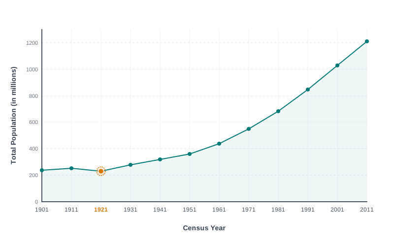
Fig. 1.0 – India’s total population, 1901–2011.
1.1 Distribution Of Population
People are the most important part of any country, and India has a great many of them. India is the second most populous country in the world after China, with a total population of 1,210 million in 2011. That single figure is larger than the populations of North America, South America and Australia added together.
A population this large is often said to press hard on the country’s limited resources and to lie behind many of its social and economic problems. It is worth pausing on what ‘India’ even means here. Is it only a stretch of territory on a map, or is it the amalgam of people who live on that territory, joined together under shared institutions of governance? For a geographer studying population, India is above all its people — and the first task is to find out how many there are and where they live.
Those numbers come from the census, a complete count of every person in the country, carried out once every ten years. India’s first census was attempted in 1872, but the first complete count was made only in 1881. Since then a census has been taken every decade, which is why almost every figure in this chapter is dated to a census year such as 2011.
An Uneven Portrait
The distribution of population is the pattern of how people are spread across space — which areas hold many and which hold few. India’s distribution is highly uneven. If you examine the dot map in Fig. 1.1, where each dot stands for 200,000 persons, you can see the dots crowd together in some regions and thin out almost to nothing in others.
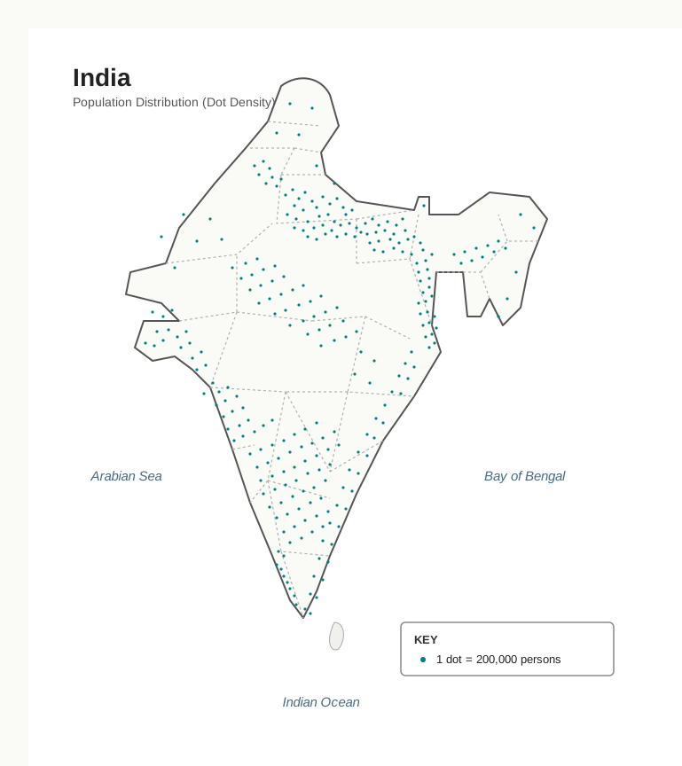
Fig. 1.1 – Distribution of population in India, 2011.
The share of population — a state’s people counted as a percentage of the national total — makes the same point in figures. Uttar Pradesh has the highest population, followed by Maharashtra, Bihar and West Bengal. Taken together with Andhra Pradesh, Tamil Nadu, Madhya Pradesh, Rajasthan, Karnataka and Gujarat, these ten states account for about 76 per cent of all the people in the country.
At the other extreme, some states hold only a tiny share despite covering a fairly large area. Jammu & Kashmir has just 1.04 per cent of the national population and Uttarakhand 0.84 per cent, while Arunachal Pradesh, in the far north-east, has only 0.11 per cent. A large map area, then, is no guarantee of a large population.
This mismatch is worth testing for yourself. Using state-level data, you can sort the states and Union Territories into three groups: those large in area and large in population, those large in area but small in population, and those small in area yet large in population. The very fact that the second and third groups exist tells you distribution and area do not move together.
Why The Pattern Is Uneven
An uneven distribution like this points to a close relationship between where people settle and the physical, socio-economic and historical conditions of a place. It helps to set the factors out as a branching chain (Fig. 1.2), because they act in two broad groups.
Among the physical factors, climate, terrain and the availability of water matter most. Where the land is level, the climate kind and water reliable, people gather; where it is not, they stay away. This is why the North Indian Plains — the broad lowland belt across the north — together with the river deltas and coastal plains carry a far higher share of population than the interior districts of the southern and central states, the Himalayas, parts of the north-east and the dry western margins.
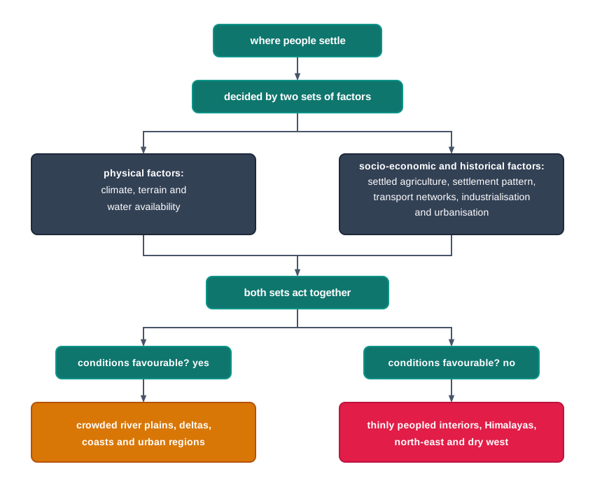
Fig. 1.2 – Factors shaping population distribution.
Physical conditions are not the whole story, and they can be overcome. The spread of irrigation in Rajasthan, in the arid north-west, has drawn people onto land that was once thinly peopled. So has the wealth of minerals and energy resources in Jharkhand, in eastern India, and the growth of transport networks across the Peninsular states. Each has raised population in places that were previously almost empty.
The socio-economic and historical factors run just as deep: the early rise of settled agriculture, long-established patterns of human settlement, the building of transport networks, and later industrialisation and urbanisation. The river plains and coastal areas were settled early and served by transport first, and so they have stayed crowded. Even where heavy use has begun to degrade their land and water, the people have not moved away.
Cities add a second layer to this pattern. The urban regions of Delhi, Mumbai, Kolkata, Bengaluru, Pune, Ahmedabad, Chennai and Jaipur hold dense concentrations of people, pulled there by industrial growth and city work, which keeps a steady stream of rural-urban migrants flowing in.
1.2 Density Of Population
Distribution tells you where people are; density tells you how thickly they are packed. Density of population is the number of persons living on each unit of area, usually a square kilometre. It sharpens the picture of distribution by tying people directly to the land they occupy.
\[\text{Density of population} = \frac{\text{Total population}}{\text{Total area}} \quad (\text{persons per km}^2)\]
Total population is the number of people counted, total area is the land they live on in square kilometres, and the result is read as persons per square kilometre — the average number of people sharing a square of land one kilometre on each side.
India’s density in 2011 was 382 persons per sq km. It has climbed steadily over the decades: from 117 persons per sq km in 1951 to 382 in 2011, an increase of more than 200 persons per sq km across those years.
The land itself has not grown; only the number of people on it has. A rising density therefore means steadily more people leaning on the same fixed area — the same fields, the same water, the same housing. That is why a high and climbing density is read as rising pressure on land, and why a single national figure, useful as it is, only opens the question rather than settling it.
Reading The Density Map
The national average hides an enormous spread. Across the country density ranges from as low as 17 persons per sq km in Arunachal Pradesh to 11,297 persons in the National Capital Territory of Delhi — the small, heavily built-up area around the capital. Fig. 1.3 shades this variation across the map.
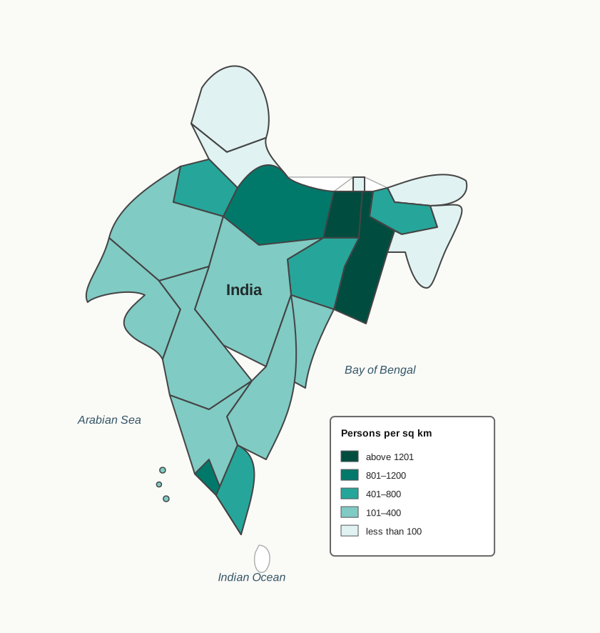
Fig. 1.3 – Population density of India, 2011.
Among the northern states, Bihar (1102), West Bengal (1029) and Uttar Pradesh (828) carry high densities. In the peninsula the highest are Kerala (859) and Tamil Nadu (555). States such as Assam, Gujarat, Andhra Pradesh, Haryana, Jharkhand and Odisha fall in the moderate range. The hill states of the Himalayan region and the north-eastern states (except Assam) have relatively low densities, while the Union Territories (except the Andaman and Nicobar islands) are very densely peopled.
A Crude Measure Refined
Plain density is a crude measure of the human–land relationship because it divides all people by all land, farmed or not. For a country with as many farmers as India, two sharper measures tell us more about the pressure of people on the land that actually grows food.
\[\text{Physiological density} = \frac{\text{Total population}}{\text{Net cultivated area}}\]
\[\text{Agricultural density} = \frac{\text{Total agricultural population}}{\text{Net cultivable area}}\]
Physiological density divides the whole population by the net cultivated area — the land actually under crops — so it shows how many people, in total, each unit of cropped land must feed. Agricultural density divides only the agricultural population by the net cultivable area — the land that can be farmed — and so it shows how heavily the farming community itself leans on its farmland. Here the agricultural population means cultivators and agricultural labourers together with their families.
The three measures answer three different questions. Plain density asks how many people share each square kilometre of the country; physiological density asks how many mouths depend on each unit of cropland; agricultural density asks how many farmers work each unit of farmable land. For a country like India, with a large population living off the land, the last two carry real weight.
1.3 Growth Of Population
Growth of population is the change in the number of people living in an area between two points in time, and its rate is given as a percentage. Growth has two components. Natural growth comes from births and deaths inside the population; induced growth comes from migration — people moving in and out. This chapter deals only with the natural growth of India’s population.
Natural growth is read from two rates. The crude birth rate is the number of births in a year for every 1,000 people, and the crude death rate is the number of deaths in a year for every 1,000 people. When births outnumber deaths, the population grows on its own, before any migration is counted.
India’s growth is measured over two spans. The decadal growth rate compares one census with the census ten years earlier; the annual growth rate is the yearly figure, which stood at 1.64 per cent in 2011. Both have been high, and for most of the last century both were rising.
A useful companion idea is population doubling time — the number of years a population would take to double itself if it kept growing at its current annual rate. The faster the annual rate, the shorter that time.
The decadal growth rate is worked out with a simple formula:
\[g = \frac{p_2 - p_1}{p_1} \times 100\]
Here \(p_1\) is the population of the base year, \(p_2\) the population of the present year, and \(g\) the growth over the decade expressed as a percentage. Table 1.1 applies this to every census from 1901 to 2011.
The two columns move differently, and it helps to see the rate on its own (Fig. 1.4).
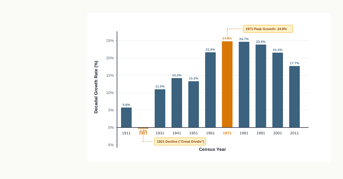
Fig. 1.4 – India’s decadal population growth rate, 1911–2011.
Four Phases Of Growth
India’s growth over the last century has been driven by the birth rate, the death rate and migration together, and it falls into four distinct phases.
Phase I covers 1901–1921, a stagnant or stationary phase. Growth was very low, and the decade 1911–1921 even recorded a fall in numbers. Birth rates and death rates were both high, so they largely cancelled each other out. Poor health and medical services, widespread illiteracy and an inefficient system for distributing food and other basics kept both rates high.
Phase II covers 1921–1951, a period of steady growth. Better health and sanitation across the country brought the death rate down, while improved transport and communication helped distribute food and goods. The crude birth rate stayed high, so growth rose above the previous phase — a striking result set against the Great Depression of the 1920s and the Second World War.
Phase III covers 1951–1981, the period of population explosion. The death rate fell rapidly while fertility stayed high, and the average annual growth rate reached as much as 2.2 per cent. After Independence, development through centralised planning improved living conditions and lifted natural increase. Increased international migration — bringing in Tibetans, Bangladeshis, Nepalis and people from Pakistan — added further to the numbers.
Phase IV runs from 1981 to the present. Growth has remained high but has begun to slow. A downward trend in the crude birth rate is held responsible, and that fall was itself driven by a rise in the mean age at marriage and by an improving quality of life, particularly the education of women.
Even with this slowing, India’s growth is still high. The World Development Report has projected that the country’s population will touch 1,350 million by 2025.
These figures describe the country’s average growth. But the average conceals a great deal: growth varies widely from one region to another, and that variation is the subject of the next section.
1.4 Regional Variation In Population Growth
The national growth rate is an average, and averages hide differences. Across the states and Union Territories, growth in the decade 1991–2001 fell into a clear pattern.
A group of states in the south grew slowly, by not more than 20 per cent over the decade: Kerala, Karnataka, Tamil Nadu, Andhra Pradesh, Odisha and Goa, along with the Union Territory of Puducherry. Kerala grew the least of all — just 9.4 per cent — the lowest rate not only in this group but in the entire country.
Against this ran a continuous belt of higher growth, stretching west to east across the north-west, north and north-central parts of the country. This belt — Gujarat, Maharashtra, Rajasthan, Punjab, Haryana, Uttar Pradesh, Uttarakhand, Madhya Pradesh, Sikkim, Assam, West Bengal, Bihar, Chhattisgarh and Jharkhand — averaged 20–25 per cent growth, well above the southern states.
The next decade brought a widespread slowing, which Fig. 1.5 maps state by state.
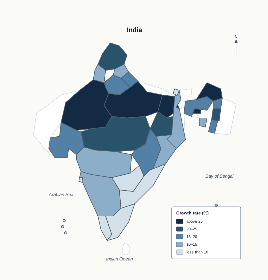
Fig. 1.5 – Decadal population growth by state, 2001–2011.
During 2001–2011, growth fell almost everywhere compared with 1991–2001. Among the six most populous states — Uttar Pradesh, Maharashtra, Bihar, West Bengal, Andhra Pradesh and Madhya Pradesh — every one grew more slowly than before. The smallest fall was Andhra Pradesh’s, 3.5 percentage points; the largest was Maharashtra’s, 6.7 percentage points. Two places moved the other way: Tamil Nadu grew 3.9 percentage points faster, and Puducherry 7.1 percentage points faster, than in the previous decade.
The pattern is worth seeing at a finer scale too. Taking district-level growth data for the male and female population of your own state, and drawing it as a composite bar graph, shows how much a single state average can conceal within its own borders.
A Youthful Population
One striking feature of India’s growth is how young the population is. Adolescents — young people aged 10 to 19 — made up about 20.9 per cent of the population in 2011. Within that group, male adolescents were 52.7 per cent and female adolescents 47.3 per cent.
This youthful population is a real strength, but it is also vulnerable if it is not supported, and the challenges should be named plainly. They include early marriage, illiteracy — female illiteracy in particular — school dropout, poor nutrition, high maternal mortality among adolescent mothers, high rates of HIV and AIDS, physical and mental disability, substance abuse, and juvenile crime.
To help young people realise their potential rather than fall to these risks, the Government of India has framed policies for their education and development. The National Youth Policy of 2014 (NYP–2014) sets out a vision to empower the youth of the country to achieve their full potential, and through them help India find its rightful place among the community of nations. The policy defines ‘youth’ as persons aged 15 to 29 — a wider band than the census category of adolescents.
The government also formulated the National Policy for Skill Development and Entrepreneurship in 2015. It provides a single framework for all skilling activities in the country, aligns them to common standards, and links training to the places where those skills are actually in demand.
Growth, then, varies widely across both space and time, and it carries real social challenges with it. To understand a population fully, however, we must look past how many people there are and how fast they grow, and ask who they are — their social composition.
1.5 Population Composition
Population composition is the make-up of a population — who its people are, sorted by their characteristics. It is a distinct field within population geography, covering age and sex, place of residence, ethnic groups and tribes, language, religion, marital status, literacy and education, and the work people do. This section looks at the composition of India’s population under four heads: rural and urban residence, language, religion, and the pattern of occupation.
1.5.1 Rural – Urban Composition
Sorting people by where they live — in villages or in towns and cities — is an important clue to their social and economic lives. It matters all the more in India, where about 68.8 per cent of the population still lived in villages in 2011.
The scale of rural India is vast. The Census of 2011 counted 640,867 villages, of which 597,608 — about 93.2 per cent — were inhabited. But rural population is not spread evenly. States such as Himachal Pradesh, in the western Himalayas, and Bihar, in the eastern Ganga plain, have a very high share of rural population, while Goa and Mizoram have only a little over half their people in villages.
The Union Territories generally have a smaller rural share, the exception being Dadra and Nagar Haveli at 53.38 per cent. Villages themselves differ hugely in size. They hold fewer than 200 persons in the hill states of the north-east, in western Rajasthan and in the Rann of Kachchh — the salt marsh of western Gujarat — but rise to as many as 17 thousand persons in Kerala and parts of Maharashtra. At every level, the degree of urbanisation and the pull of rural-urban migration shape how rural population is concentrated.
The Faster-Growing Towns
By contrast, the urban share of the population, at 31.16 per cent, is low — but it is growing much faster than the rural share, decade after decade. That acceleration comes from stronger economic development and from better health and hygiene in the towns. Urban population, like total population, varies widely across the country; comparing state data lets you pick out the states and Union Territories with very high and very low urban shares.
Almost everywhere, urban population has risen considerably, reflecting both the growth of towns and a rising tide of rural-urban migration. This migration is most visible along the road and rail corridors of the North Indian Plains and around the industrial belts of Kolkata, Mumbai, Bengaluru–Mysuru, Madurai–Coimbatore, Ahmedabad–Surat, Delhi–Kanpur and Ludhiana–Jalandhar. Where farming has stagnated — in the middle and lower Ganga plains, Telangana, non-irrigated western Rajasthan, the remote hilly and tribal north-east, the flood-prone tracts of Peninsular India and eastern Madhya Pradesh — urbanisation has stayed low.
1.5.2 Linguistic Composition
India is a land of extraordinary linguistic diversity. According to Grierson’s Linguistic Survey of India (1903–1928), the country held 179 languages and as many as 544 dialects. In modern India there are about 22 scheduled languages, together with a large number of non-scheduled ones. You can see some of this diversity for yourself by counting how many languages appear on a ten-rupee note.
Among the scheduled languages, Hindi has the largest share of speakers, while the smallest groups are the speakers of Sanskrit, Bodo and Manipuri (2011). Language regions, though, do not stop at sharp lines. They gradually merge and overlap along their frontier zones, so one linguistic region shades into the next rather than ending abruptly.
1.5.3 Linguistic Classification
The speakers of India’s major languages belong to four language families, each of which splits into sub-families and then into branches or groups. Table 1.2 sets this out, and Fig. 1.6 shows the same structure as a branching tree.
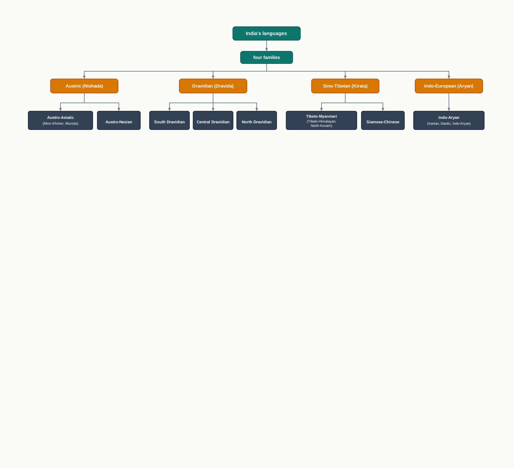
Fig. 1.6 – Classification of modern Indian languages.
From the table you can see the scale of each family: the Indo-European (Aryan) family covers about 73 per cent of speakers, the Dravidian family about 20 per cent, while the Austric and Sino-Tibetan families are far smaller, at 1.38 and 0.85 per cent. A useful exercise is to turn these shares into a pie diagram, or to map the families onto India as a symbol map to see where each is spoken.
1.5.4 Religious Composition
Religion is one of the strongest forces shaping the cultural and political life of most Indians. Because it runs through so much of family and community life, its composition is worth studying closely. Across the country, some states and districts hold a large strength of one religion, while that same community may be barely present elsewhere.
Hindus form the major group in many states, often 70 to 90 per cent or above, except in districts along the Indo-Bangladesh and Indo-Pak borders, in Jammu & Kashmir, in the hill states of the north-east, and in scattered parts of the Deccan Plateau and the Ganga plain. Muslims, the largest religious minority, are concentrated in Jammu & Kashmir, certain districts of West Bengal and Kerala, many districts of Uttar Pradesh, in and around Delhi, and in Lakshadweep — and they form a majority in the Kashmir valley and in Lakshadweep.
The Christian population is largely rural, concentrated along the western coast around Goa and Kerala, and in the hill states of Meghalaya, Mizoram and Nagaland, the Chota Nagpur area of eastern India, and the hills of Manipur. Sikhs are gathered in a comparatively small area, chiefly Punjab, Haryana and Delhi.
Jains and Buddhists, the smallest religious groups, are concentrated in only a few areas. Jains are found mainly in the urban centres of Rajasthan, Gujarat and Maharashtra, while Buddhists cluster mostly in Maharashtra, with other pockets of Buddhist majority in Sikkim, Arunachal Pradesh, Ladakh in Jammu & Kashmir, Tripura, and Lahaul and Spiti in Himachal Pradesh. India’s other religions include Zoroastrians and various tribal and indigenous faiths, scattered in small pockets across the country.
1.5.5 Composition Of Working Population
By economic status, India’s population is divided into three groups: main workers, marginal workers and non-workers. The census draws the line between the first two by time worked in the year.
In 2011, workers of both kinds together made up only 39.8 per cent of the population, leaving about 60 per cent as non-workers. That large non-working share points to a heavy dependent population, and possibly to many people who are unemployed or under-employed.
The work participation rate is the share of the population that is working. Across the states and Union Territories it ranges from about 29.1 per cent in Lakshadweep to about 51.9 per cent in Himachal Pradesh. Larger shares of workers are found in Himachal Pradesh, Sikkim, Chhattisgarh, Andhra Pradesh, Karnataka, Arunachal Pradesh, Nagaland, Manipur and Meghalaya, and among the Union Territories in Dadra and Nagar Haveli and in Daman and Diu. Oddly, participation tends to be higher where economic development is lower, because subsistence activities need many hands doing manual work.
Farming Still Leads
Occupational composition means the kind of work a person does — farming, manufacturing, trade, services or any profession. India’s is dominated by the primary sector. About 54.6 per cent of all workers are cultivators and agricultural labourers, only 3.8 per cent are in household industries, and 41.6 per cent are ‘other workers’, a wide group covering non-household industry, trade, commerce, construction, repair and other services. The 2011 Census itself sorted workers into four categories: cultivators, agricultural labourers, household industrial workers, and other workers. In every one of the three broad sectors, male workers outnumber female workers (Fig. 1.7 and Table 1.4).
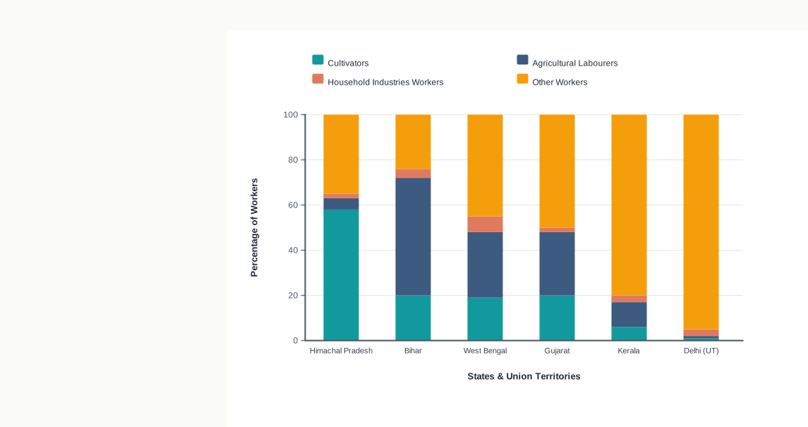
Fig. 1.7 – Occupational structure of India by state, 2011.
The gender gap becomes clearer when the table’s own figures are worked through.
Women make up a far larger slice of farm work than of service work: as jobs move from the fields to offices and factories, their share shrinks. This is what ‘male workers outnumber female workers in all three sectors’ looks like once you do the arithmetic, and it shows where the gap in paid work is widest. The number of female workers is relatively high in the primary sector, though in recent years women’s participation in the secondary and tertiary sectors has improved somewhat.
A Shifting Workforce
This uneven position of women is part of a wider question of gender in the economy. The division of society into male, female and transgender is often treated as natural, but many of the roles attached to it are social constructs, reinforced by institutions until they harden into discrimination and exclusion. Shutting out over half the population is a serious handicap to any society, a point the UNDP made when it warned that ‘if development is not engendered it is endangered’ (HDR UNDP 1995). To confront the denial of education, employment, fair wages and dignity, the Government of India launched the nationwide ‘Beti Bachao – Beti Padhao’ campaign.
The overall balance of work is also changing. The share of workers in agriculture fell from 58.2 per cent in 2001 to 54.6 per cent in 2011, while the secondary and tertiary sectors gained. This marks a real shift of dependence from farm-based to non-farm work — a sectoral shift in the economy itself. Comparing composite bar graphs of male and female workers for India and for your own state, across agriculture, household industries and other sectors, brings this shift into focus.
The pattern varies sharply across space. States like Himachal Pradesh and Nagaland have very large shares of cultivators, while Bihar, Andhra Pradesh, Chhattisgarh, Odisha, Jharkhand, West Bengal and Madhya Pradesh carry higher proportions of agricultural labourers. The heavily urbanised areas of Delhi, Chandigarh and Puducherry have large shares of workers in other services — a sign both of limited farmland and of large-scale urbanisation and industrialisation pulling workers into non-farm jobs.
1.6 Summary
- India is the second most populous country in the world, with 1,210 million people in 2011, counted by a census taken once every ten years.
- Population is very unevenly distributed: about ten states, led by Uttar Pradesh, hold roughly 76 per cent of all Indians, a pattern set by physical, socio-economic and historical factors.
- Density, the number of persons per square kilometre, rose from 117 in 1951 to 382 in 2011, and ranges from 17 in Arunachal Pradesh to 11,297 in Delhi.
- Plain density is a crude measure; physiological and agricultural densities give a sharper picture of the pressure of people on cultivable land.
- Population growth has natural and induced components; this chapter treats natural growth, whose annual rate was 1.64 per cent in 2011.
- Growth passed through four phases over the last century, and though still high, it has been slowing since 1981 as the birth rate falls.
- Growth varies by region — lowest in the south, where Kerala grew just 9.4 per cent in 1991–2001, and higher across a north-to-north-central belt — with almost all states slowing during 2001–2011.
- Adolescents made up about 20.9 per cent of the population in 2011, a youthful group that is both a strength and a responsibility.
- About 68.8 per cent of Indians were rural in 2011, but the urban share, though smaller, is growing much faster.
- India is richly diverse in language, with four language families of which the Indo-European is the largest, and in religion, with Hindus the majority and Muslims the largest minority.
- Only 39.8 per cent of the population are workers; of these, 54.6 per cent are in the primary sector, though work is shifting toward non-farm jobs, and male workers outnumber female workers in every sector.
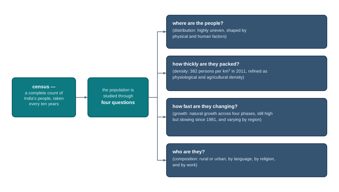
Fig. 1.8 – The four key questions of population study.
What This Chapter Cannot Tell You
The chapter works almost entirely with national and state averages, and averages hide as much as they reveal. A state density or growth figure smooths over the crowded city and the empty district inside the same state, just as a national religious or linguistic share hides the places where a small minority is a local majority.
Its numbers are also snapshots. A decadal growth rate says nothing about how change was spread across the ten years, and a census portrait ages the moment it is taken. The count can tell us how many people there are, where they live and what work they do — but not why an individual migrated, married later, or changed their faith. And the projection to 1,350 million by 2025 holds only for as long as today’s trends do.
1.7 NCERT Questions
- India’s population as per 2011 census is:
- 1028 million
- 3182 million
- 3287 million
- 1210 million
- Which one of the following states has the highest density of population in India?
- West Bengal
- Kerala
- Uttar Pradesh
- Bihar
- Which one of the following states has the highest proportion of urban population in India according to 2011 Census?
- Tamil Nadu
- Maharashtra
- Kerala
- Goa
- Which one of the following is the largest linguistic group of India?
- Sino – Tibetan
- Indo – Aryan
- Austric
- Dravidian
- Very hot and dry and very cold and wet regions of India have low density of population. In this light, explain the role of climate on the distribution of population. (30 words)
- Which states have large rural population in India? Give one reason for such large rural population. (30 words)
- Why do some states of India have higher rates of work participation than others? (30 words)
- ‘The agricultural sector has the largest share of Indian workers.’ – Explain. (30 words)
- Discuss the spatial pattern of density of population in India. (150 words)
- Give an account of the occupational structure of India’s population. (150 words)
1.8 Check Your Concepts
- Table 1.1 shows one census decade in which India’s population actually fell. Name that decade, say which growth phase it belongs to, and give the reason the chapter offers for the fall.
- In Fig. 1.1 each dot represents 200,000 persons. Describe what the clustering of dots in some regions and their near-absence in others tells you, and state one thing a dot map cannot tell you about how crowded a single town is.
- Distinguish between a main worker and a marginal worker as the 2011 Census defines them.
- The chapter says climate, terrain and water shape where people settle. Apart from these physical factors, what socio-economic and historical factors does it give for the uneven distribution of India’s population?
- Using the figures in Table 1.4, work out what share of primary-sector workers were women in 2011, and say how this compares with women’s share of tertiary-sector workers.
- Plain density is described in the chapter as a ‘crude’ measure. Explain why, and show how physiological density and agricultural density give a sharper picture of land pressure for a country like India.
- Reconstruct the four phases of India’s population growth in order, giving one defining feature of each, and explain what turned the trend after 1981.