Chapter 9: Introduction to Bioinformatics

In the early 1960s, protein chemistry was moving faster than paper could keep up with. Every few months, some laboratory would finally work out the amino acid sequence of one more protein and publish it in a journal. Each sequence then sat alone inside its own article. Nobody could easily lay two of them side by side and ask the obvious question: do these two proteins, taken from two different species, look like relatives?

Margaret Oakley Dayhoff, an American physical chemist who had earned her doctorate in chemistry at Columbia University, thought this was a waste of hard-won information. She had spent her career applying mathematics and computational methods to biochemistry, in a period when computers filled whole rooms and instructions were fed in on punched cards. Her idea was simple, and for its time radical: gather all the known protein sequences into one place, written in one common format, so that anyone could compare them.

In 1965 she published the Atlas of Protein Sequence and Structure, an open, comprehensive collection of protein sequences. It became the model on which the sequence databases that came later were built. She also devised the one-letter codes for amino acids that biologists still use every day, for a very practical reason — shorter codes meant smaller data files, and the computers of that era could barely manage anything larger.

Dayhoff had seen something before almost anyone else. Biology was about to become a science of data, and data must be organised before it can be made to mean anything.

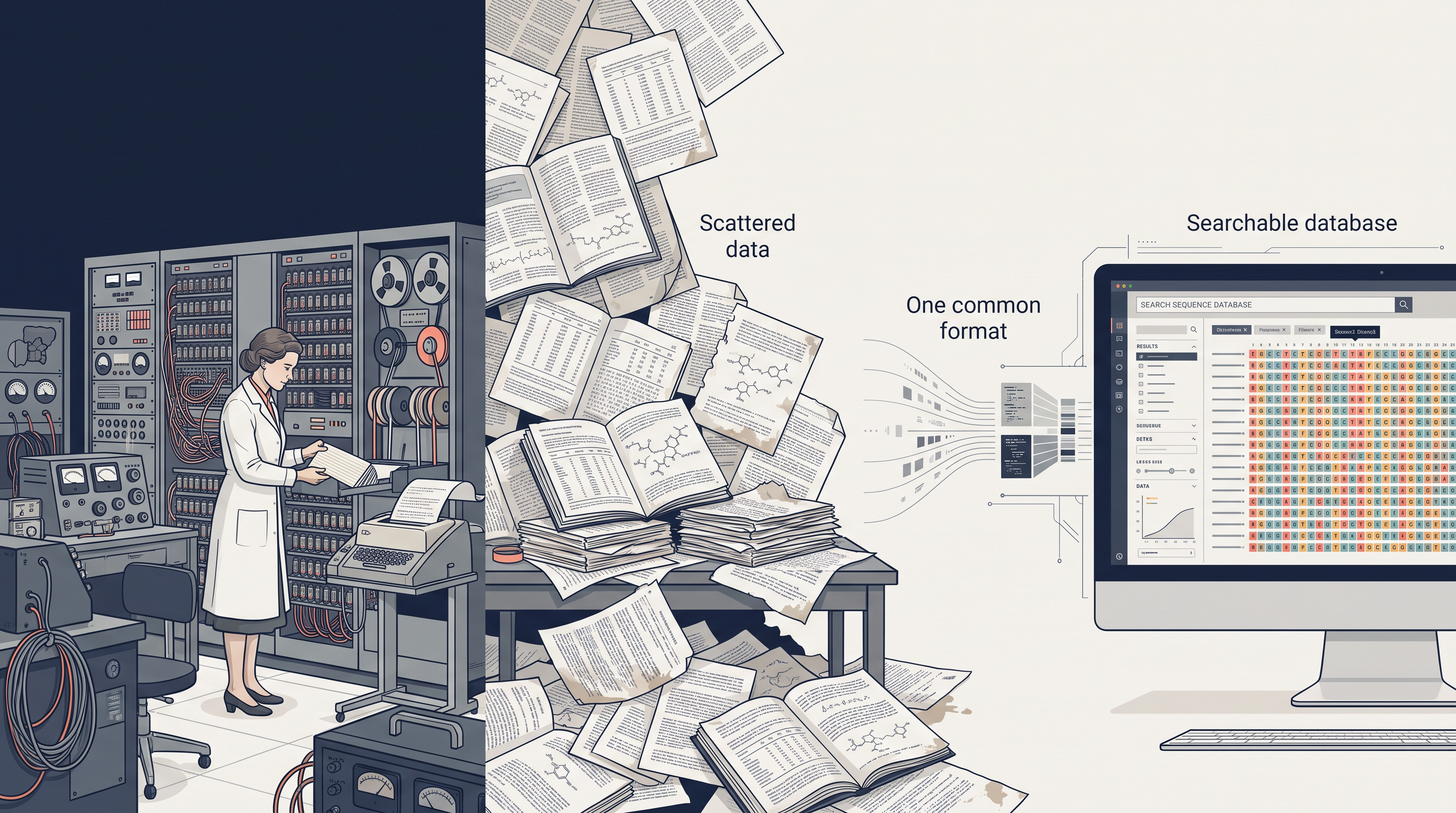
Fig. 9.0 – The transition from scattered records to searchable databases.

Curiosity Corner

Q1. Why can a modern biologist no longer manage the results of an experiment with just a notebook and a spreadsheet? Q2. If two things in the body seem to rise together — say heart rate and blood pressure — how does a scientist show that the link is real and not just something the eye imagines? Q3. How is a DNA sequence stored so that a computer anywhere in the world can search through it in seconds? Q4. The human genome was announced as complete in 2003, so why do scientists still say that parts of it are missing? Q5. Can a machine that learns on its own take over the job of interpreting biological data?

Keep these five questions in mind as you read — this chapter will answer every one of them.

9.1 The Utility of Basic Mathematical and Statistical Concepts to Understand Biological Systems and Processes

Before we open the subject of bioinformatics, one idea has to be settled first: a biologist today cannot work well without a working understanding of mathematics and statistics. That is the purpose of this opening section. It is not asking you to become a mathematician. It is asking you to see why numbers have become part of the everyday equipment of a life scientist.

Data Is the Real Product of an Experiment

Think about what an experiment actually produces. Not a conclusion — a conclusion is something you build later. What an experiment produces is data: readings, counts, images, sequences, intensities. Every biological experiment, from a simple germination trial to a genome sequencing run, ends in data.

For a long time, biologists generated and analysed that data on their own, without sophisticated software, computational tools or statistical tests. The volumes were small enough that a careful person with a notebook could handle them. That era has ended.

Instruments changed the scale of the problem. High-throughput DNA sequencers, powerful microscopes and other imaging systems, and analytical instruments capable of producing very large volumes of data now deliver more numbers in a single run than a researcher could examine by hand in a lifetime. A biologist can no longer manage such output with a notebook and an Excel sheet. Computational and statistical tools have become necessary, not optional.

There is a second reason, and it matters more than the first. Large volumes of data need quantitative analysis before they will yield any biological meaning at all. A million sequencing reads sitting in a file say nothing. Only when they are counted, compared, and tested do they begin to say something about a gene, a disease or an organism.

Curiosity Corner

Q1. Why can a modern biologist no longer manage the results of an experiment with just a notebook and a spreadsheet?

A. Because modern instruments — high-throughput sequencers, imaging systems and analytical machines — generate data in volumes far beyond what a person can read, sort or compare by hand. Extracting biological meaning from that much data requires quantitative analysis, which needs computational and statistical tools.

Carrying out such analyses requires a good working knowledge of computational and statistical concepts — machine learning technologies, regression, variance, and correlation, among others. But here comes a warning that you should carry through the whole chapter. Mathematical and statistical concepts can only aid a biologist in interpreting data. They are not a replacement for asking the right question in the first place, and they are not a replacement for biological acumen — the trained judgement that tells you whether a result makes biological sense. A perfectly executed statistical test on a badly framed question gives a perfectly meaningless answer.

Some of the statistical terms you will meet repeatedly in biology are collected below.

Side Note

Glossary of commonly used statistical terms in biology

Null hypothesis — A statement that there is no relationship between two measured phenomena.

Statistical significance — A result has statistical significance when it is very unlikely to have occurred.

p-value — The probability of finding the observed results when the null hypothesis of a study question is true.

t-test — An analysis of two population means through the use of statistical examination.

Multivariate analysis — A set of techniques used for analysis of data that contain more than one variable.

Regression analysis — A technique to investigate the relationship between a dependent and an independent variable.

Multiple testing correction — A statistical test that corrects for multiple tests to keep the overall error rate to less than or equal to the user-specified P-value cutoff.

Analysis of Variance or ANOVA — A collection of statistical models used to analyse the differences among group means in a sample.

Seeing a Pattern Is Not Proving One

Let us take a specific example where computing and statistics together help us understand a biological phenomenon better. Suppose we want to know whether there is any association between blood pressure and heart rate. We record both in ten patients, as given in Table 9.1.

Table 9.1: Heart rate and blood pressure recorded in ten patients

Patient	Heart rate	Blood pressure (systolic)
1	112	189
2	83	140
3	92	153
4	121	192
5	85	147
6	111	178
7	94	135
8	88	143
9	102	177
10	111	189

Read down the two columns and a pattern seems to appear — patients with higher heart rates seem to have higher blood pressure. But “seems to” is exactly the problem. A simple visual estimation, even after the points are plotted as in Fig. 9.1, is not sufficient to determine the relationship — the correlation — between the two variables accurately. The human eye is very good at inventing patterns that are not really there. For a dependable answer, one needs to draw a regression line through the points.

Fig. 9.1

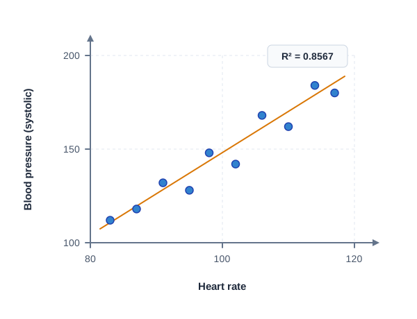
Fig. 9.1 – Scatter plot of blood pressure against heart rate.

Correlation and regression are distinct ideas, though they are themselves closely connected. Correlation quantifies how the two variables are connected — how tightly they move together. Regression goes further and defines a statistical relationship between two or more variables, in which a change in one variable is associated with a change in another.

Definition

Correlation is a measure of how closely two measured variables are connected to each other.

Definition

Regression is a statistical relationship defined between two or more variables, in which a change in one variable is associated with a change in another.

So, in the example above, a simple regression test will tell us whether there is a direct relationship between heart rate and blood pressure.

Reading the R² Value

The output of a linear regression analysis is the \(R^2\)-value. It is a statistical measure that shows how close the data points lie to the fitted regression line. Its value ranges from \(0\), meaning no correlation between the variables, to \(1\), meaning perfect correlation between the variables:

\[0 \leq R^2 \leq 1\]

A value near \(0\) means the points are scattered so widely that the line explains almost nothing. A value near \(1\) means the points hug the line closely, and knowing one variable tells you a great deal about the other.

Definition

The \(R^2\)-value of a linear regression is a statistical measure of how close the data are to the fitted regression line, ranging from 0 (no correlation between the variables) to 1 (perfect correlation between the variables).

As shown in Fig. 9.1, the \(R^2\) value obtained here is \(R^2 = 0.8567\). This suggests that there is a good correlation between the two variables. Remember that our starting position — the null hypothesis — was that heart rate and blood pressure have no relationship. The data do not support that position. Therefore, the null hypothesis is rejected in this case.

Notice the logic carefully, because it is the shape of almost every statistical argument in biology. You do not begin by trying to prove your idea. You begin by assuming there is no effect, and then ask whether the data make that assumption untenable.

Technique

Simple linear regression Principle: If two variables are genuinely related, the points plotted against each other will cluster around a straight line; fitting the best possible line and measuring how tightly the points hug it converts a visual impression into a number. Steps: State the null hypothesis (no relationship) → plot the dependent variable against the independent variable → fit the best-fit straight line through the points → calculate \(R^2\) → judge whether \(R^2\) is high enough, and the result significant enough, to reject the null hypothesis. Used for: Testing whether one measured variable is associated with another — for example, whether systolic blood pressure rises with heart rate, or whether a crop’s yield rises with fertiliser dose.

Curiosity Corner

Q2. If two things in the body seem to rise together — say heart rate and blood pressure — how does a scientist show that the link is real and not just something the eye imagines?

A. By fitting a regression line through the plotted data and calculating the \(R^2\) value. A high \(R^2\), such as the 0.8567 obtained for the ten patients in Table 9.1, shows the points lie close to the line, which allows the null hypothesis of “no relationship” to be rejected on evidence rather than on impression.

Numerical 9.1

A student fits a linear regression line to two data sets. Data set A gives \(R^2 = 0.91\) and data set B gives \(R^2 = 0.23\). (i) In which data set do the points lie closer to the fitted line? (ii) Express, as a percentage, how much of the variation is accounted for by the fitted line in each case. (iii) Which data set gives stronger grounds for rejecting the null hypothesis, and why?

Compare Table

Why Probability Runs Through Biology

Many fields of biology require a basic understanding of probability. Mathematical modelling of complex systemic phenomena, such as cellular mechanisms, allows one to understand the vital parameters of the system and its kinetics — that is, which quantities actually drive the system and how fast it moves.

Probability is equally central to evolutionary work. Phylogenetic reconstruction, determining ancestral sequences, and modelling rates of evolution from a collection of extant sequences all require knowledge of probability. This is unavoidable: an ancestral sequence no longer exists to be measured, so it can only be inferred as the most probable sequence given the sequences that survive today.

Statistics Before the Experiment, Not After

Biologists need to settle statistical issues before performing an experiment, not after the data are in. Choosing an adequate number of samples and of replicates — both biological and technical — requires knowledge of statistics. A biological replicate is an independent biological sample; a technical replicate is a repeated measurement of the same sample. Too few of either, and no amount of later analysis will rescue the experiment.

An experiment must be repeated multiple times independently to build confidence in the results and to know whether they are real or false. A necessary background in statistical randomness and in the law of large numbers equips a biologist to deal with this problem. Random sampling from a large number reduces the chance of obtaining biased results, because it prevents any hidden preference from creeping into which individuals are chosen.

The biologist must then make sure that the results are statistically significant. This step requires familiarity with the various tests and measures of statistical significance, and the judgement to apply the correct test to the problem in question. Depending on the problem, the biologist may also have to correct and adjust the measure of significance for multiple testing — because when you run many tests at once, some will appear significant purely by chance.

Fig. 9.2

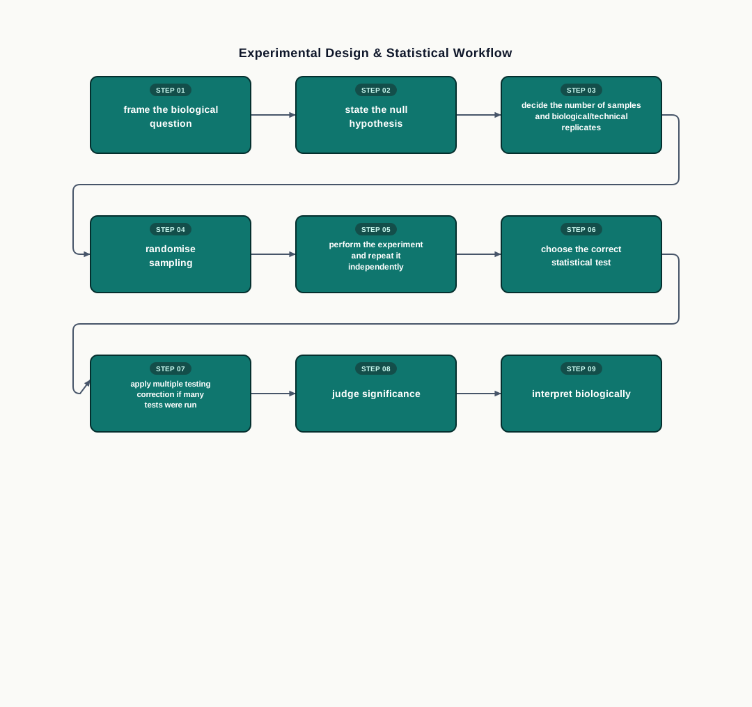
Fig. 9.2 – Planning a statistically sound biological experiment.

The full sequence, from question to interpretation, is summarised in Fig. 9.2. Notice that the statistical thinking sits at both ends — before a single reading is taken, and again after.

Tools for Higher-Level Computing

For higher levels of computing, analysis and visualisation, a biologist can use built-in frameworks such as MATLAB, which is commercial, and R, which is open source. These are environments in which statistical procedures and graphics are already written and tested, so the biologist can concentrate on the biological question rather than on writing the mathematics from scratch.

The Choice of Test — and the Traps

For biologists, the choice of the statistical analysis employed is the key to arriving at the right answer. Weak or incorrect statistical standards lead to false assumptions and may therefore lead to irreproducible results — results that no other laboratory can obtain again.

Take the most commonly used concept in statistics, the P value, used as evidence of support for a hypothesis. The smaller the P value, the more likely it is that the result of the test is significant. A P value cutoff of \(0.05\), which corresponds to \(95\%\) significance, or less, is conventionally considered significant.

However, that convention has a cost. The \(0.05\) threshold has caused too many false positives to appear in the scientific literature. The P value cutoff of \(0.05\) therefore needs to be re-examined rather than applied automatically.

Sample size brings its own trap. With small sample sizes, one is better off showing all the independent data points rather than distorting the visualisation with a misleading average and standard deviation. Four data points averaged into a single bar can conceal the fact that two of them disagreed completely.

There is also an asymmetry that researchers fall into. Statistical power — the ability of a test to detect a real effect if one exists — is something a researcher readily thinks about when faced with a negative result, wondering whether the experiment was simply too small to see the effect. It should be considered just as carefully in the case of a positive result.

Applying the assumptions of established statistical models and distributions to the wrong type of data is, for this reason, a common abuse. For example, assuming a Gaussian distribution for nonlinear dynamical systems produces false positives, because the data simply do not have the bell-shaped behaviour the model expects. Unbalanced mathematical models constructed with unrealistic parameter weights are yet another common abuse — and a particularly dangerous one, because they are difficult to detect from the outside.

With due consideration to all these caveats, the application of mathematics and statistics to biology can open up newer areas of research that are inter-disciplinary in nature, and equip us to tackle far more complex biological problems than biology alone could handle.

How This Section Is Tested

In board and competitive examinations, this material rarely appears as a plain definition question. It appears as data interpretation — you are given a scatter plot or a small table like Table 9.1 and asked what the \(R^2\) value implies, or whether the null hypothesis should be rejected. It also appears as assertion–reason items, where the assertion states a conclusion and the reason states a statistical justification, and you must decide whether the justification actually supports the conclusion.

Try Yourself

Look at Table 9.1 again. Patient 4 has the highest heart rate and also the highest blood pressure, while Patient 7 has a heart rate of 94 but a blood pressure of only 135 — lower than Patient 2, whose heart rate is just 83. Does this single mismatched patient disprove the relationship? Write two sentences explaining why one deviating point does not overturn a regression result.

9.2 Introduction

Bioinformatics is an interdisciplinary field that uses computational, mathematical, statistical and, occasionally, engineering approaches to analyse biological information in order to solve biological problems. The word “interdisciplinary” is doing real work in that sentence — it means the subject genuinely sits at the meeting point of several disciplines, as shown in Fig. 9.3, rather than belonging to any one of them.

Fig. 9.3

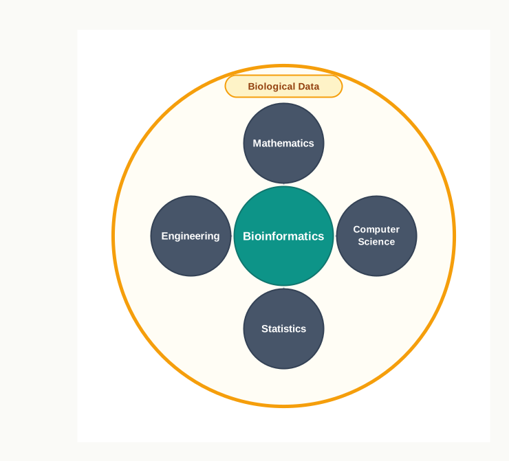
Fig. 9.3 – Inter-disciplinary nature of bioinformatics.

Put more practically, bioinformatics deals with the storage, retrieval, analysis and interpretation of biological data using computer-based software and tools. Those four words — storage, retrieval, analysis, interpretation — are worth remembering, because the rest of this chapter is organised around them.

Definition

Bioinformatics is an interdisciplinary field that applies computational, mathematical, statistical and sometimes engineering approaches to the storage, retrieval, analysis and interpretation of biological data, in order to solve biological problems.

A Word With Several Neighbours

You will meet other names for work that looks very similar. Although there are differences between them, bioinformatics is used alternatingly and interchangeably with terms such as computational biology, mathematical biology, quantitative biology and bio-statistics, depending on which disciplinary component happens to dominate a particular piece of work.

It must be noted, however, that the use of these definitions varies among experts and practitioners, and has changed with time. This is not a flaw in your understanding — it is a genuine feature of a young, fast-moving field. A study heavy in modelling may be called mathematical biology by one group and computational biology by another, and both may be right.

Exam Corner

Q. If the boundaries between these terms are blurred, how should a student handle a question asking for “the” definition of bioinformatics?

A. Give the operational definition — an interdisciplinary field that stores, retrieves, analyses and interprets biological data using computational tools to solve biological problems — and then note that related terms overlap with it depending on which discipline dominates. That is exactly how practitioners themselves treat it.

9.2.1 Historical perspective

Bioinformatics aids in the discovery of new findings through data mining, and also in the generation of new hypotheses. Data mining simply means searching through very large collections of existing data for patterns that nobody has yet noticed. Both of these — new findings and new hypotheses — are achieved through the modelling or analysis of molecular data.

Most bioinformatics tools work on one of two kinds of input. The first is pre-existing nucleotide and protein data drawn from sequence and structure databases. The second is newly created data generated using high-throughput instruments such as next-generation sequencers and DNA microarrays. In other words, a bioinformatician either mines what has already been deposited by others, or processes what an instrument has just produced in the laboratory.

Where the Data Came to Live

The National Center for Biotechnology Information (NCBI) in the USA was created, in the late 1980s, as a resource for bioinformatics tools and services. It houses nucleotide databases, protein databases, bibliographic databases and more, and remains the single most-used doorway into biological data anywhere in the world.

GenBank, a widely used database that stores all publicly available DNA sequences, was launched in 1982. Notice the order of events — GenBank came before the term “bioinformatics” was in common use, which tells you that the practice existed before the name did.

Real Incident / Discovery

The word “bioinformatics” has a surprisingly short written history. Although the work was being practised long before the term spread, it was not until 1991 that “bioinformatics” began appearing in the scientific literature. The name gained wide acceptance only after the launch of the Human Genome Project, when bioinformatics tools were used extensively for the analysis of sequence data and the discipline suddenly became visible to every biologist. The use of the term in the literature is therefore not more than about thirty years old — younger than most of the techniques it describes.

Bioinformatics gained broader attraction in the post-genome-sequencing and high-performance-computing era, following advances in — and easier access to — both biotechnology and computing technology. Before this, when the focus was on lower-throughput assays such as studying the action of a single gene or studying morphology under a microscope, bioinformatics was still used, but on a much smaller scale. The subject did not appear from nowhere; it scaled up.

Structure Came Before Sequence

Here is a point that examiners are fond of, because it reverses the order most students assume. Structural bioinformatics precedes informatics based on high-throughput genome-wide assays such as sequencing and DNA microarrays.

The reason is historical. Studies on the three-dimensional structures of proteins, using NMR spectroscopy and X-ray crystallography, began in the early 1900s. Genome informatics and the other “-ome” informatics — the informatics of whole collections of molecules — were introduced only in the early 2000s and are continuing to develop to this day. Protein structures were being solved, stored and compared while whole-genome sequencing was still out of reach.

Compare Table

The number of Protein Data Bank (PDB) structures and of GenBank entries grows every year, and neither shows any sign of levelling off.

The Central Job, and Its Difficulties

The primary concern in bioinformatics is to manage sequence and structural data in the form of databases, and then to mine data from those databases to obtain biological meaning. Storage without mining would be a warehouse nobody visits.

NCBI hosts both nucleotide and protein data under various categories such as Gene, Genome, Structure and Sequence. Currently, biological data are being produced at an unprecedented rate, and their analysis and interpretation — the step that leads to critical biological insight — have taken on higher priority than the mere act of generating more data. To meet this, new, optimised and superior algorithms and tools, with statistical adaptations and synthesis drawn from multiple fields, are constantly being developed and implemented.

Databases have grown beyond raw sequence too. Databases based on secondary and tertiary levels of information have since been developed and used, covering molecular pathways, gene expression, protein structure and function, interaction networks, disease-associated changes, organism specificity and regulatory networks. A “secondary” database, in this sense, holds information derived by analysis rather than measured directly.

Bioinformatics is an evolving field, and part of that evolution is correction. Because biological data are dynamic, because gene and exon–intron boundaries shift as knowledge improves, and because sequences carry discrepancies, in silico translation errors are common and are continually being updated. Here in silico means “performed on a computer”, the counterpart of in vivo and in vitro. Such errors include frameshift errors, annotation errors, assembly errors, and simple spelling mistakes. A database entry is therefore not a permanent fact; it is the current best record, open to revision.

We will now look at the different types of biological molecules, the kinds of data produced by the techniques that assay them, and the analytical and statistical workflows commonly used to interpret and visualise that data. The whole path is summarised in Fig. 9.4. Details of the experimental techniques used for the production of genomic data are described in Unit V.

Fig. 9.4

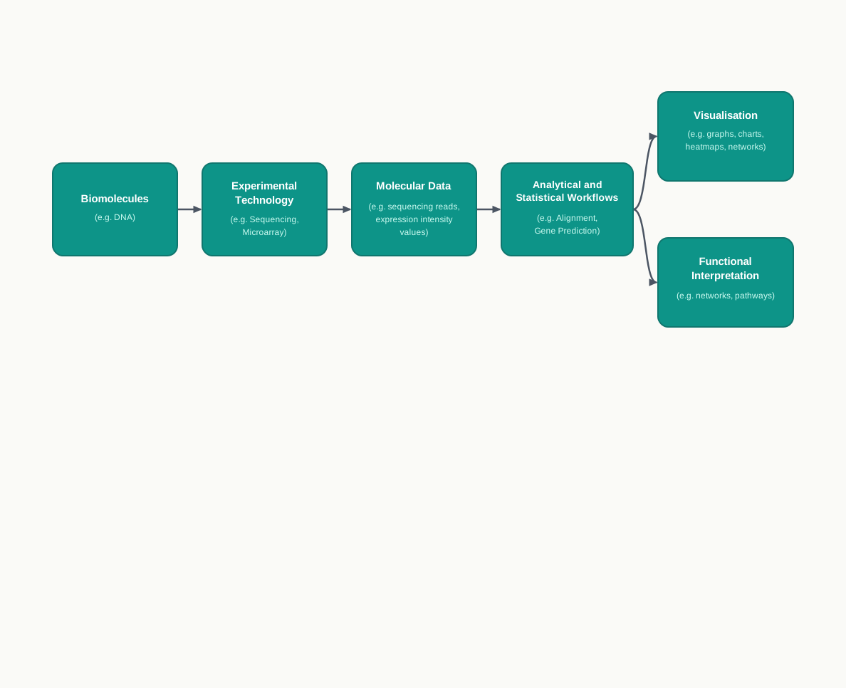
Fig. 9.4 – The pathway from biomolecules to function.

Read Fig. 9.4 from left to right as a chain of conversions. A biomolecule is a physical object; an experimental technology turns it into numbers or letters; an analytical workflow turns those into a claim; and visualisation and functional interpretation turn the claim into something a biologist can act on. Every stage that follows in this chapter fits somewhere on that chain.

9.2.2 Types of experimental technologies for analysing biomolecules

A few critical experimental technologies used for the identification and/or quantification of biomolecules are given in Table 9.2. Details on some of these techniques are described in Unit V; for now, what matters is the pairing — which technology is applied to which biomolecule, and to answer what question.

Table 9.2: Name of the technology, biomolecules assayed and the purpose of the technology

Technology	Biomolecule	Purpose
PCR (Polymerase Chain Reaction)	DNA	Amplify a region of interest
RT (Real-Time)-PCR/qPCR (quantitative PCR)	RNA	Detect RNA expression
Next-generation sequencing	DNA/RNA	To sequence genes/genomes and RNA
Gel electrophoresis	DNA, RNA and Proteins	Separation of fragments, based on their size and charge
HPLC (High-performance Liquid Chromatography)	Metabolites	Separation, identification and quantification of metabolites
MS (Mass spectrometry)	DNA, proteins, metabolites, trace gases	Fragmentation, measurement of isotopic composition and mass determination
EM (Electron microscope)	DNA, RNA or protein	Structure, and sequence determination

Notice the logic of the third column. Each technology answers a different type of question. PCR asks “can I get more of this piece of DNA?” Real-time PCR asks “how much of this RNA is present?” Sequencing asks “what is the exact order of bases?” Gel electrophoresis asks “how big are these fragments?” HPLC and mass spectrometry ask “what small molecules are here, and in what amounts?” Electron microscopy asks “what does it look like?”

The first two rows are the pair most often confused in examinations, so it is worth separating them clearly.

Compare Table

9.2.3 Types of molecular data

Different technologies assay different biomolecules, and each therefore produces a different type of data output, delivered in its own format. Some are plain text; some are images; some are binary files a human cannot read at all without software. Examples are collected in Table 9.3.

The descriptions of the two commonly used DNA data formats, FASTQ and FASTA, are provided later in this chapter, in Genome Informatics. For the moment, simply note how different the outputs of the various technologies look.

Table 9.3: Types of molecular data and their formats

Technology	Molecular data formats	Examples
Next-Gen Sequencing	Reads (.fastq)	`@read1` `TTTCCGGGGCCCATAATCTTCTGCAG` `+` `8C;=<=;9@4368>9:67AA<9>63<`
Microarray	.cel, intensity data files (.idat), reports, binary file	PROBE_ID Assay_Name_1.QT1 Assay_Name_1.QT2 Assay_Name_2.QT1 Assay_Name_2.QT2
Capillary Gel Electrophoresis based Sequencing (Sanger)	.chromat, .fasta, .ab1	`>seq1 TCACCTTCTGGGATCCAG` and a chromatogram trace
High performance Liquid chromatography (HPLC)	Chromatogram	A plot of absorbance unit (254 nm) AU against time in minutes, showing separated peaks
Mass spectrometry (MS)	Mass spectrum	A plot of relative abundance against mass, showing peaks at characteristic values

Two of the rows in Table 9.3 are graphs rather than text, and reading them is a skill in itself. In an HPLC chromatogram, the horizontal axis is time in minutes and the vertical axis is absorbance measured at 254 nm; each peak marks a compound emerging from the column at its own characteristic time, and the size of the peak relates to how much of it there is. In a mass spectrum, the horizontal axis is mass and the vertical axis is relative abundance; each line marks a fragment of a particular mass, and the pattern of fragments acts as a fingerprint for the parent molecule.

9.2.4 Commonly used analytical and statistical workflows

Biological knowledge may or may not be mandatory for merely running an open-source or proprietary tool — many tools will execute happily for anyone who can type the command. However, biological knowledge is essential for asking relevant questions and for interpreting biological results, exactly as was said at the beginning of this chapter.

This leads to a working rule you should carry into any laboratory. Before using any tool, one must understand its logic and principle, and be aware of the assumptions that underlie its working. A tool that assumes your sequences are related will happily align two sequences that are not; a tool that assumes a particular error profile will mislead you on data produced by a different instrument.

Commonly Used Analysis Tools

Some commonly used analysis tools are as follows:

Homology search (Basic Local Alignment Search Tool (BLAST) – blastn, blastp)
Sequence alignment (CLUSTAL, MAFFT, MUSCLE)
Phylogenetics (PHYLIP, PAUP)
Gene prediction (GlimmerHMM, GenScan)
Functional homology search (HMMER)
RNA structure (mfold, sFold, uniFold)
Regulatory region analysis (MatInspector, BEARR, RSAT)
Protein structure (Phyre2, Jpred)

You are not expected to memorise every name in that list, but you should be able to match a category to a purpose. Homology means similarity due to shared ancestry, so a homology search asks “has anyone seen a sequence like mine before?” Sequence alignment lines several sequences up so that matching regions sit in the same columns. Phylogenetics builds evolutionary relationships from those alignments. Gene prediction locates genes inside raw sequence. Regulatory region analysis looks for the control switches that sit outside genes.

Statistical Packages Behind the Tools

Bioinformatics tools use various statistical and computational algorithms and approaches. Some commonly used statistical packages are:

Statistical Package for the Social Sciences (SPSS)
Statistical Analysis System (SAS)
R
Microsoft Excel

R appears here as a statistical package for exactly the reason it appeared earlier as a computing framework — it is one environment that serves both purposes, which is a large part of why biologists have adopted it so widely.

From Findings to Function

At the final stages of biological data analysis, gene- and protein-level findings are linked to certain functions. This is the step where a computational result becomes a biological claim.

These functional interpretations can be made using commonly used biological tests such as loss-of-function or gain-of-function assays, gene knockouts, and gene editing. The reasoning behind them is direct: if removing a gene removes a trait, or adding it produces the trait, the gene is implicated in that function. Additionally, by inferring affected networks and pathways using computational tools, one can assign functional significance to a gene and to its protein product.

Fig. 9.5

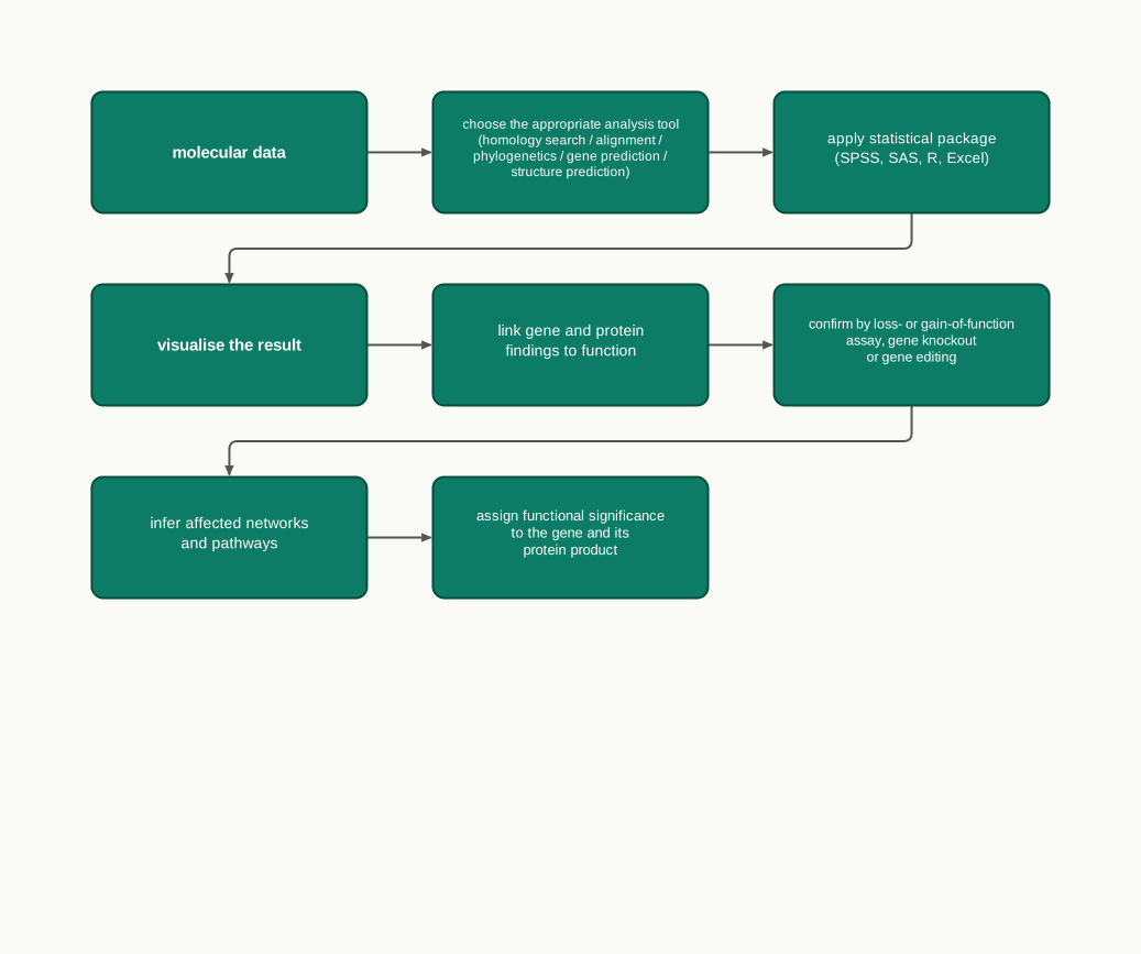
Fig. 9.5 – From molecular data to functional significance.

The whole route from a data file to a functional claim is summarised in Fig. 9.5. Compare it with Fig. 9.4 and you will see they describe the same journey — Fig. 9.4 in terms of the kinds of thing involved, Fig. 9.5 in terms of the order of operations.

Try Yourself

Pick any one row of Table 9.2 and trace it across Fig. 9.4. Name the biomolecule, the experimental technology, the kind of molecular data it would produce, and one analytical tool from the list in 9.2.4 that could reasonably be applied to that data.

9.3 Biological Databases

A biological database is a repository that contains an organised, structured and searchable collection of biological data. Put more simply, it is a library of biological information that is easy to reach into and easy to search.

Each of those three words carries weight. Organised means the data are arranged rather than dumped. Structured means every entry has the same set of fields, so a computer knows where to look. Searchable means a question can be asked of the whole collection at once.

Definition

A biological database is a repository containing an organised, structured and searchable collection of biological data, which links all the relevant data to their original creators or to a reference describing the underlying data.

A good database never presents data as though it appeared from nowhere. A biological database links all its relevant data back to the original creators, or to a reference that describes the underlying data. This is what makes an entry checkable — if a sequence looks wrong, you can trace it to the laboratory and the publication it came from.

Where the Contents Come From

The information held in a database is collected in two ways: through experiments, and through computational approaches. Both kinds of entry can sit side by side, which is why a database record often distinguishes what was actually measured from what was predicted by software.

Consider a database of human genes as an example. It contains both the actual nucleotide sequence of all the genes and their characteristics — the sequence itself, and the descriptive information that gives that sequence meaning.

Databases also differ in who builds them. A database can be made by a single group of researchers collecting information from a variety of public resources, or it can be built by multiple teams of researchers who each add data to a single shared repository.

What a Biological Database May Store

A biological database may store several different types of information. Among them are:

the primary nucleotide sequence of a gene;
mutations in a given gene that are specific to a disease, and the frequency of single nucleotide polymorphism (SNP) in various populations;
the translated protein sequence of the genes;
the 3D structures of proteins and domains;
the functional interaction of one protein with another.

A single nucleotide polymorphism is a position in the genome where a single base commonly differs between individuals of a population. Recording how often each version occurs, population by population, is what allows a clinician to judge whether a base change found in a patient is an ordinary variation or something rare enough to be worth investigating.

What Makes a Database Good

Not every collection of data deserves to be called a good database. The characteristics of a good biological database are that it:

is easy to access and use;
has a user-friendly interface;
has excellent documentation;
has support staff who can answer queries from its users;
lacks errors in the underlying data;
is cross-referenced;
continually updates its information as and when the primary source is updated.

The last two deserve a moment’s thought. Cross-referencing means that a gene entry points outward to the protein it encodes, to the structure of that protein, and to the literature describing it, so that a user is never trapped inside one database. Continual updating matters because, as you saw in the previous section, biological data is dynamic — an entry that is never revised slowly becomes wrong.

Fig. 9.6

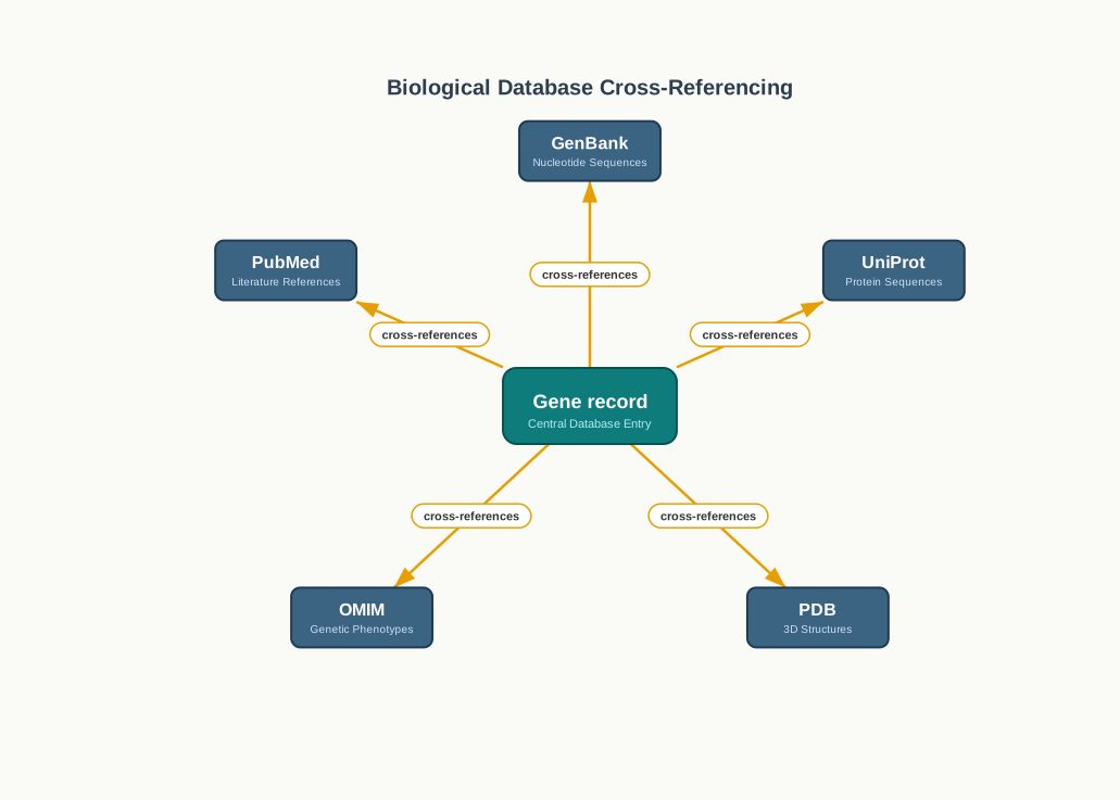
Fig. 9.6 – Cross-referencing between biological databases.

Follow the arrows in Fig. 9.6 in either direction. That two-way traffic is the practical meaning of cross-referencing, and it is why a biologist can begin with a disease name and end at an atom-by-atom protein structure without ever typing a sequence by hand.

How Databases Are Organised and Managed

There are two main types of databases: relational and non-relational.

Databases are managed by using a software system called a database management system (DBMS), which is used to manipulate, retrieve and manage data. The DBMS sits between the user and the stored data — the user never touches the raw files.

Definition

A database management system (DBMS) is the software system used to manipulate, retrieve and manage the data held in a database.

The structured query language (SQL) is the standard application program interface for a relational database. In practice this means SQL is the agreed language in which a question is put to a relational database, so that a query written by one person can run on a database built by another.

A non-relational or NoSQL database does not follow the order of a relational database, and is used for large sets of distributed and unstructured data. “Unstructured” here means data that does not fit neatly into fixed rows and columns — images, free text, raw instrument output — and “distributed” means the data may be spread across many machines rather than sitting in one place.

Compare Table

Fig. 9.7

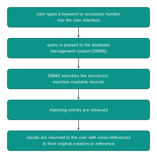
Fig. 9.7 – How a database query is answered.

9.3.1 What Is the Need for a Biological Database?

Scenario

Imagine walking into your school library and asking the librarian for a particular book. What if the librarian had to physically walk to every shelf and look for it? That would take a long time, and even then there would be no guarantee of finding the book. Now imagine instead that the librarian searches a database that stores every book in the library, typing in a keyword from the title, or the author’s name, or both. The job becomes much simpler, and much more reliable.

That is exactly why we need databases — to make the search process easy and foolproof.

But biological data raises a difficulty that a library does not. In a library, the items are physical and can be seen with the open eye; a book is an object you can pick up. Nucleotide sequences, genes and protein structures are tiny, and they cannot be searched for physically at all. There is nothing to walk up to and look at.

Therefore, the information must be encoded and stored in a machine-readable format inside a database that can be easily searched using a user interface. Encoding is the crucial step: a sequence of bases is written as a string of letters that a computer can compare, count and match at speed.

Curiosity Corner

Q3. How is a DNA sequence stored so that a computer anywhere in the world can search through it in seconds?

A. The sequence is encoded as text in a standard machine-readable format and deposited in an organised, structured biological database. A database management system then searches those structured records on request through a user interface, so a query is answered by comparing text rather than by examining any physical material. The exact text formats used for DNA are described later in this chapter.

With the exponential growth of biological data — especially genome data from various organisms, alongside information on their functions and interactions — it has become imperative to store biological information in databases. The growth is not gradual but exponential, which is why manual record-keeping stopped being an option rather than simply becoming inconvenient.

Some Commonly Used Biological Databases

GenBank (https://www.ncbi.nlm.nih.gov/genbank/): A collection of annotated publicly available DNA sequences.
PDB (www.wwpdb.org): A collection of 3D structures of proteins, nucleic acids, and complex assemblies.
UniProt (www.uniprot.org): A collection of protein sequences and function.
PubMed (https://www.ncbi.nlm.nih.gov/pubmed/): A collection of biomedical literature.
KEGG (www.kegg.jp): A collection of biological pathways, diseases, drugs, and chemical substances.
OMIM (www.omim.org): A catalog of human genes and genetic disorders.

Learn these by what they hold rather than by their names alone — sequences in GenBank, structures in PDB, proteins in UniProt, literature in PubMed, pathways in KEGG, human genetic disorders in OMIM. Questions on this material almost always ask you to match a database to the kind of data it stores.

In addition to the above, there are organism-specific databases, disease-specific databases and secondary databases, all of which are used routinely by biologists.

Bioethics

Depositing human genomic data in public databases Public databases work because scientists agree to make their data open, and this openness is the reason a laboratory in one country can build on results obtained in another. Human data, however, is not like the sequence of a bacterium. A person’s genome carries information about their disease risks, and about the disease risks of their relatives, who never consented to anything. On one side stands the clear public benefit: shared SNP frequencies and disease-associated mutations are what allow a clinician to interpret a patient’s variant at all, and withholding data slows the diagnosis of rare disorders for everyone. On the other side stand privacy and consent, since genetic information cannot be made anonymous in the way a name can be removed from a form. The usual safeguard is a two-tier arrangement — summary information such as population-level variant frequencies is made openly available, while individual-level genomic records are placed in controlled-access repositories that researchers may use only with approval and under conditions set by the participants’ consent.

9.3.2 Data Visualisation

Biological data visualisation is an essential aspect of bioinformatics. Its purpose is straightforward: a table of a million numbers tells a human being nothing, while a well-made picture of the same numbers can reveal a pattern in a moment.

Visualisation involves the application of graphics and of data representation, and it incorporates sequences, genomes, alignments, phylogenies, macromolecular structures, microscopy images, and other imaging information. In other words, almost every kind of data met so far in this chapter has a matching way of being drawn.

A few examples of data visualisation tools and their uses are provided in Table 9.4.

Table 9.4: Data visualisation tools and their uses

Visualisation tool	Use
UCSC Genome browser (https://genome.ucsc.edu/)	An online interactive website to visualise macro- and micro-level genome information on vertebrate and invertebrate species.
KEGG (http://www.genome.jp/kegg/pathway.html), Biocarta (http://www.biocarta.com), Reactome (https://reactome.org/)	Visualisation of pathways.
CIRCOS (circos.ca/)	Visualisation of data in circular layout.
EXCEL	Histograms, scatter plots, bubble charts, heat maps
R (https://www.r-project.org/)	A software environment for statistical computing and generating graphics.
D3.js (https://d3js.org/)	A JavaScript library for producing dynamic, interactive data visualisations in web browsers.
Phinch (phinch.org/)	An interactive, exploratory framework for visualising biological data.
Integrative Genomics Viewer (IGV, http://software.broadinstitute.org/software/igv/)	A visualisation tool for interactive exploration of large, integrated genomic datasets.

Notice that KEGG appears twice in this chapter — once as a database of pathways, diseases, drugs and chemical substances, and again here as a tool for viewing those pathways. That is common in bioinformatics: the same resource both stores the data and draws it.

Exam Corner

Q. Two tools in Table 9.4 both let you look at genomic data — the UCSC Genome browser and CIRCOS. Why would anyone choose the circular layout?

A. A genome browser lays a chromosome out as a straight line, which is ideal for zooming in on one region. A circular layout places all the chromosomes around a ring, so links drawn across the middle of the circle can show relationships between distant parts of the genome at a glance — which is why circular plots are preferred for displaying variants and rearrangements across a whole genome at once.

Try Yourself

For each of the following needs, name one suitable resource from this section and say why: (i) you want the published papers on a gene, (ii) you want the three-dimensional structure of the protein it encodes, (iii) you want to see which metabolic pathway that protein belongs to, (iv) you want to display variants from a whole genome in a single circular figure.

9.4 Genome Informatics

Genome

Everything in this section rests on one word, so we begin by fixing it precisely.

A genome is the complete set of DNA of an organism, including its genes and the intergenic regions. Note that the intergenic regions — the stretches lying between genes — are part of the genome. A genome is not a list of genes; it is all of the DNA, gene and non-gene alike.

Definition

The genome is the complete set of DNA of an organism, including its genes and the intergenic regions.

Genomics is the field of science that deals with the structure, function, evolution, mapping, and modification of genomes.

Definition

Genomics is the field of science dealing with the structure, function, evolution, mapping and modification of genomes.

Genome informatics is the application of bioinformatics tools to process the outputs of genome-wide assays and technologies, facilitating the interpretation of the data and linking them to function. Read that carefully and you will see the whole purpose of this section inside it: process the output, interpret it, and connect it to what the organism actually does.

Definition

Genome informatics is the application of bioinformatics tools to process the outputs of genome-wide assays and technologies, so that the resulting data can be interpreted and linked to function.

Genomics is one of the omics fields, the other commonly used terms being transcriptomics, proteomics and metabolomics. Each of these studies one whole class of molecules at once rather than one molecule at a time — genomics the whole genome, transcriptomics all the transcripts, proteomics all the proteins, metabolomics all the metabolites. All of these fields have evolved rapidly over the last decade.

How Genome Information Is Obtained

Genome information is obtained using high-throughput methods or assays, carried out on instruments that provide information on several different things:

the DNA/RNA nucleotide sequence;
the variations in genomes;
changes in gene expression;
the profiles of regulatory protein binding to DNA/RNA;
DNA/RNA methylation and various other profile changes.

Details on these methods are provided in Unit V.

The term high-throughput relates to a process that produces a significant amount of data. It is a statement about volume, not about accuracy — a high-throughput instrument is one that delivers a great deal of data in a single run.

Definition

A high-throughput method is one that produces a significant amount of data in a single process or run.

The Scale of the Problem

The amount of data generated by genome sequencing is substantial, and it is worth pausing on how substantial. Some of the large genome centres in the world, such as the Broad Institute of the Massachusetts Institute of Technology (MIT) and Harvard, produce more than 24 TB of genome data per day. Furthermore, the magnitude of such data being generated is increasing continuously, day by day.

There are not many large genome institutes like the Broad, so this figure is not typical of every laboratory. It is quoted to give you a sense of the magnitude of genome data being produced nowadays. In fact, it has been postulated that the computing resources required to handle genome data will exceed those involved in processing Twitter and YouTube data.

Because the amount of data is so significant, genome data needs the power of computer science, information technology, quantitative methods and analytics, and statistics if we are to gain any understanding of the underlying complexity, patterns and meaning. This is the argument of Section 9.1 arriving in its most concrete form.

Numerical 9.2

A genome centre produces 24 TB of genome data per day. (i) How much data does it produce in one week? (ii) How much in a year of 365 days, expressed in TB? (iii) If a single portable hard disk stores 2 TB, how many such disks would be needed to hold one day’s output?

9.4.1 Human Genome Project

An initiative to sequence the complete nucleotide content in human cells started in the early 1990s. This initiative is known as the Human Genome Project.

The sequencing method proposed and used by Fred Sanger was used, with modifications, by both of the major efforts involved. One was the publicly funded initiative headed by the National Human Genome Research Institute (NHGRI) of the National Institutes of Health, USA. The other was the private company Celera Genomics.

Real Incident / Discovery

Both efforts set out to read the same genome, and both built on Fred Sanger’s sequencing method — yet they used different strategies to get there. The publicly funded initiative sequenced human DNA that had first been cloned into bacterial artificial chromosomes, so that every piece being read was already tied to a known region of a chromosome. Celera Genomics took the opposite approach and sequenced randomly cut human DNA, letting a computer work out afterwards how the pieces fitted together. This second technique is called the whole-genome shotgun sequencing method. The public effort’s approach was slower but kept its bearings throughout; the shotgun approach was faster but placed the entire burden of reconstruction on computation — which is precisely why the Human Genome Project became the event that made bioinformatics indispensable.

Technique

Whole-genome shotgun sequencing Principle: If genomic DNA is broken at random into many fragments and each fragment is sequenced, the fragments will overlap one another; those overlaps contain enough information for a computer to reconstruct the original order without knowing it in advance. Steps: Cut the whole genome randomly into fragments → sequence the fragments → detect overlaps between the sequenced fragments computationally → assemble the overlapping fragments into longer continuous stretches → build up the draft genome sequence. Used for: Sequencing whole genomes rapidly without first mapping every piece to a chromosome — the strategy used by Celera Genomics for the human genome.

Compare Table

Why the Genome Is Still Not Finished

The first complete draft human genome was published in 2001. The project then announced the release of the entire human genome in 2003. Even so, it remains an unfinished task, because the human genome sequence available today still has many gaps where the sequence information is not known.

The reason lies in the structure of chromosomes themselves. Most of the sequenced part of the genome lies in the euchromatic regions of the chromosomes, with minimal representation from the heterochromatic regions. Euchromatin is loosely packed and gene-rich; heterochromatin is tightly packed and gene-poor.

The heterochromatic areas mainly consist of repetitive elements and are primarily located in the centromeric and telomeric regions of the chromosomes. These regions are difficult to assay with the current sequencing technology.

There is a second, purely computational difficulty. Because the DNA there is repetitive, such sequences are difficult to assemble to a single location in the chromosome unambiguously. Imagine being handed a thousand identical jigsaw pieces — each one fits in a thousand places, so no arrangement can be shown to be the right one.

Exam Corner

Q. If a repeat sequence occurs in a hundred places in the genome, why can’t the assembly software simply place it in the first available position?

A. Because the resulting genome would be a guess presented as a fact. Placing a repeat in the wrong location shifts everything around it, and any later analysis — gene prediction, variant calling, comparison with another genome — would inherit that error. Leaving a gap is scientifically honest; a confident wrong answer is not.

Curiosity Corner

Q4. The human genome was announced as complete in 2003, so why do scientists still say that parts of it are missing?

A. Because the sequence available today still contains many gaps. The parts that were sequenced well lie mostly in the euchromatic regions. The heterochromatic regions — largely repetitive, and concentrated near centromeres and telomeres — are hard to assay with current sequencing technology, and their repetitive nature makes it impossible to assemble them unambiguously to a single position on a chromosome.

9.4.2 Commonly Used Data Format

One of the standing challenges of bioinformatics is working with the different formats in which data arrives. If every instrument wrote its output in its own private style, no tool could read another tool’s results. The bioinformatics community therefore adopts a standard data format for data from the same analytes.

For example, most DNA sequencing data from high-throughput DNA sequencers — with some exceptions — is presented in the FASTQ format. FASTQ is a text-based format that stores sequence information along with its corresponding quality scores. Both the sequence letter and its corresponding quality score are encoded with a single ASCII character each.

That single-character encoding is a deliberate piece of design, and it echoes Margaret Dayhoff’s reason for inventing one-letter amino acid codes: one character per base, one character per quality score, means the smallest possible file for a very large amount of information.

The sequence information inside a FASTQ record uses the FASTA format, which is a text-based format for representing sequence information in single-letter codes, as shown in Fig. 9.8. An example of a FASTA file and of a FASTQ file is given in Table 9.3.

Reading a FASTA File

The first line in a FASTA file usually starts with a > (greater-than) symbol and holds a summary description of the sequence. This description is often a unique library accession number, or the name of a gene. Everything after that first line is the sequence itself, written in single-letter codes.

A typical header line looks like this:

>K02382.1 Human growth hormone synthetic gene, complete cds

Read across it and you can see four distinct pieces of information packed into one line: the accession number, the identifier or gene name, the source, and the type of sequence.

Fig. 9.8

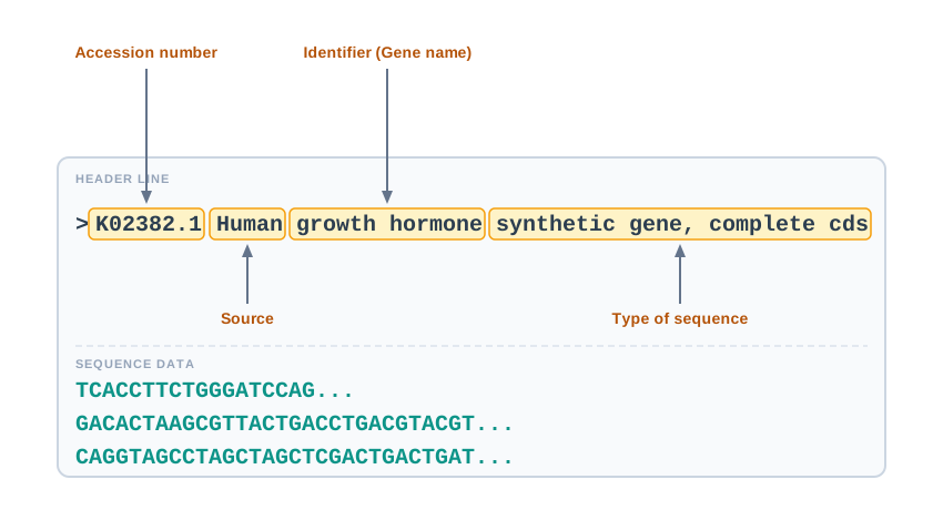
Fig. 9.8 – Structure of the FASTA format.

Reading a FASTQ File

A FASTQ file typically uses four lines per sequence, and each line has a fixed job:

Line 1 begins with an @ character, followed by the sequence description.
Line 2 contains the raw sequence letters.
Line 3 begins with a + character.
Line 4 shows the quality values for the sequence given in line 2.

There is one rule that ties lines 2 and 4 together, and it is the most commonly tested detail of the whole format: the quality values in line 4 contain the same number of symbols as there are letters in the sequence presented in line 2. This must be so, because every single base needs its own quality score. If the two lines differ in length, the record is corrupt.

Additionally, both line 1 and line 3 may include optional sequence identifiers.

In line 4, which represents quality values, the character ! represents the lowest quality and the character ~ represents the highest quality.

Compare Table

Numerical 9.3

A FASTQ record has 150 letters in line 2. (i) How many symbols must line 4 contain? (ii) If a sequencing run produces 40 million such reads, how many bases of raw sequence does the run generate in total? (iii) If a read is trimmed so that only the first 120 bases are retained, what percentage of the original read length is discarded?

9.4.3 Genome Informatic Tools

Genome informatics tools came up in parallel with the development of sequencing technology, in order to cater to the analysis of the resulting data. Neither could have been useful without the other — a sequencer with no analysis software produces unreadable files, and analysis software with no sequencer has nothing to read.

High-throughput sequencing instruments produce sequence reads, which are either short, about 100–150 nucleotides, or long, running to a few kilobases, depending on the target size and the device used. A read is simply one continuous stretch of sequence as reported by the instrument.

Two Modalities of Analysis

Once the reads are in hand, they must be organised into something meaningful, and there are exactly two ways to do it. The resulting sequenced reads need to be either assembled into a genome, where no prior genome information is known, or aligned to a reference genome, in the case of re-sequencing.

Broadly, therefore, there are two possible analytical workflows:

One based on aligning the reads to a reference sequence, such as a known genome.
One based on the de novo assembly of the reads into a draft reference genome sequence.

The choice is not a matter of taste. If a good reference genome for that organism already exists, aligning to it is faster and more reliable. If no genome has ever been sequenced for that organism, there is nothing to align to, and assembly is the only option.

Compare Table

Quality Control Comes First

In both scenarios, the sequencing data is pre-processed and checked for quality before anything else is attempted. The tools used are listed in Table 9.5.

Table 9.5: Quality Control tools for pre-processing of raw sequencing data

Tool category	Examples of tools	Function
QC (Quality control)	FastQC	To QC high-throughput sequence data
QC (Quality control)	Trimmomatic	Quality and adaptor trimming

Adaptors are short synthetic sequences attached to DNA fragments during library preparation. They are part of the laboratory procedure, not part of the organism, so leaving them in the data would place artificial sequence into the assembled genome. Trimming removes both these adaptors and the low-quality ends identified from the FASTQ quality line.

Skipping quality control is the classic beginner’s error. Every later step — assembly, alignment, gene prediction — treats its input as true, so poor-quality bases do not announce themselves later; they quietly become wrong conclusions.

Assembling Reads into Contigs

The de novo assembly-based workflow involves assembling a genome by piecing together reads on the basis of their overlaps and their insert size, which is the distance between paired-end reads. Overlaps tell the software which reads belong next to each other; insert size tells it roughly how far apart two ends of the same fragment should lie, which helps span awkward regions.

A simplified demonstration of the assembly of reads into a contiguous stretch, called a contig, is provided in Fig. 9.9. Follow the three stages in the figure: a scatter of sequenced reads at the top, the same reads arranged so that their overlapping portions line up in the middle, and a single continuous stretch at the bottom.

Fig. 9.9

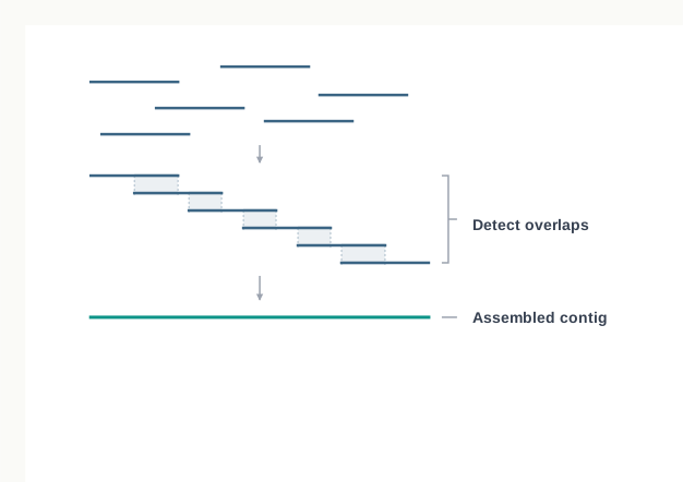
Fig. 9.9 – Assembly of reads into a continuous stretch (contig).

Technique

De novo assembly Principle: Reads drawn at random from a genome will overlap one another; where two reads share an identical end region, they almost certainly came from the same place in the genome, so overlaps can be used to rebuild the original sequence with no reference at all. Steps: Pre-process and quality-check the reads → detect overlaps between reads → also use insert size between paired-end reads → merge overlapping reads into contigs → order and process the contigs into a draft genome → annotate the assembly. Used for: Building a draft reference genome for an organism that has never been sequenced before.

The assembly then undergoes further annotation and processing. This includes the prediction of novel genes; the identification of genes based on homology to already known ones; the quantification of gene expression; and the identification of splice variants, novel isoforms, and fused transcripts.

The whole route, from an instrument’s raw output to a usable genome, is summarised in Fig. 9.10.

Fig. 9.10

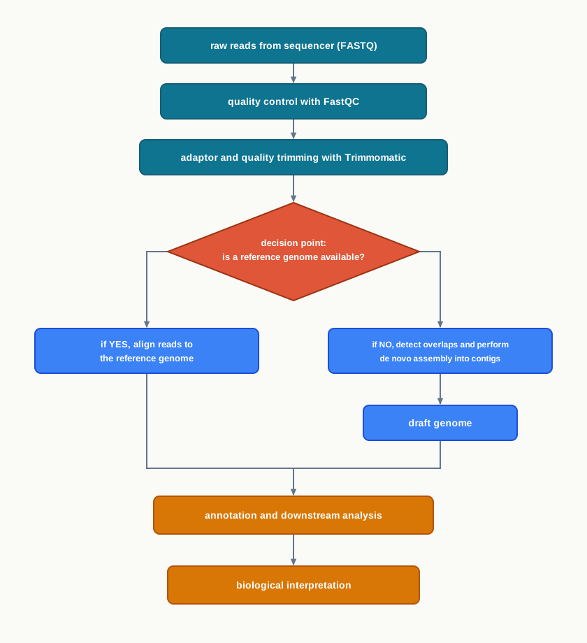
Fig. 9.10 – Sequencing data analysis workflow.

Conversion and Auxiliary Tools

There are several conversion and auxiliary tools used for the downstream analysis of genome data. A few of them are highlighted in Table 9.6.

Table 9.6: Conversion and auxiliary tools used in the analytical workflow

Category	Sub-category	Tool	Function
Aligners	Database search	Basic Local Alignment Search Tool (BLAST) – blastn, blastp	Search nucleotide or protein query sequence against non-redundant sequence database
Aligners	Database search	BLAST-like alignment tool (BLAT)	Stores the genome index in memory; designed to quickly find highly similar sequences (>95%), of at least 40 nucleotides
Aligners	Pairwise alignment	BLAST (bl2seq)	Allows comparison of one sequence against the other
Aligners	Pairwise alignment	CLUSTAL	Series of multiple sequence alignment programs
Aligners	Pairwise alignment	MUltiple Sequence Comparison by Log-Expectation (MUSCLE)	Better speed and accuracy than CLUSTAL and T-Coffee
Aligners	Pairwise alignment	Tree-based Consistency Objective Function For alignment Evaluation (T-Coffee)	Progressive approach; supports the use of PDB files; in its advanced versions can identify motifs
Conversion tools	SAM tools	—	SAM (Sequence Alignment/Mapping) to BAM (Binary Alignment/Mapping) conversion
Conversion tools	PICARD tools	—	SAM to Fastq

The conversion tools deserve a word, because their purpose is easy to miss. SAM is a text format for alignments and BAM is its binary equivalent — the same information, stored compactly for a machine rather than legibly for a person. Converting text to binary saves a great deal of space and makes the file far quicker to read, which matters when a single alignment file may run to many gigabytes.

Technique

BLAST (Basic Local Alignment Search Tool) Principle: Two sequences that share a common evolutionary origin will contain short stretches of near-identical letters; by first locating these short matches and then extending them outwards, a query sequence can be compared against an entire database far faster than by comparing it end-to-end with every entry. Steps: Submit the query sequence → choose the program according to the sequence type (blastn for nucleotide, blastp for protein) → the tool searches the non-redundant sequence database → short matching regions are found and extended into local alignments → hits are returned ranked by how good the match is. Used for: Finding out what an unknown sequence resembles — for example, identifying a newly sequenced gene by its similarity to a characterised gene in another organism.

Compare Table

9.4.4 Downstream Analyses, Interpreting Data and Linking to Function

Having a sequence is not the same as understanding it. The steps below are what turn a string of letters into biology.

Genome Annotation

Genome annotation is the process of identification and classification of all the features in a genome. After a genome is assembled, it is analysed in order to predict and identify the locations of the coding parts of genes, the exon–intron junctions, repeat elements, non-coding elements, and pseudogenes.

Definition

Genome annotation is the process of identifying and classifying all the features present in a genome.

Repeats are a significant component of any eukaryotic genome, and it would be a mistake to dismiss them as junk. They provide diversity to individual genomes, and they could play a significant role in genome evolution.

Repeats in a genome are classified into three major categories:

Transposons
Satellites
Low complexity regions

Out of these, transposons form the most significant chunk of repeat elements.

Gene Prediction

Gene prediction involves the identification of all the coding sequence in a genome. The tools used for gene prediction may follow one of three models — ab initio, similarity-based, or integrated.

Definition

Gene prediction is the identification of all the coding sequences present in a genome.

The ab initio approach works from first principles, using the statistical features of the sequence itself. The similarity-based approach instead uses sequence similarity for identifying coding regions: programs like BLAST and its sub-packages are used to carry out an exhaustive comparative search using existing, already-known sequences. The reasoning is simple — if a stretch of your new genome closely resembles a gene already characterised in another organism, it is very probably a gene.

The last approach, the integrated model, utilises both strategies and integrates the gene prediction results obtained from each of these two methods.

Exam Corner

Q. Why would anyone use the ab initio approach when similarity search seems easier and more reliable?

A. Because similarity search can only find genes that resemble something already in the databases. A gene unique to that organism, or one whose relatives have never been sequenced, has nothing to be similar to — and would simply be missed. The ab initio approach can still detect it from the sequence’s own features, which is exactly why the integrated model, using both, is the strongest option.

Gene Ontology

After gene prediction, the gene products and their associated functions need to be integrated and represented without ambiguity. This is a real problem: two laboratories may describe the same function in two different phrases, and a computer cannot tell that they mean the same thing.

The Gene Ontology aims to describe gene products in terms of their associated biological processes, cellular components, and molecular functions. Those three categories are the standard vocabulary — what process the product takes part in, where in the cell it acts, and what it does at the molecular level.

Definition

The Gene Ontology is a system that describes gene products in terms of their associated biological processes, cellular components and molecular functions, so that the same function is always described in the same unambiguous way.

Transcript Prediction

Prediction of transcripts, both coding and non-coding, is important for understanding the identity of unannotated genes and transcripts — those stretches that have been sequenced but not yet described.

There are several tools that can do this. For example, Cufflinks, cuffmerge and cuffcompare are part of a suite that helps in the identification of transcripts.

Phylogenetic Analysis

Phylogenetic analysis is done to determine the evolutionary relationship, or phylogeny, of an organism with others.

This relationship can be expressed as a diagram called a cladogram or phylogenetic tree. On such a diagram, the distance of an organism indicates how closely that organism is related to the others on an evolutionary scale — the shorter the distance, the closer the relationship.

Definition

A cladogram or phylogenetic tree is a diagram expressing the evolutionary relationship between organisms, in which the distance between organisms indicates how closely they are related on an evolutionary scale.

Fig. 9.11

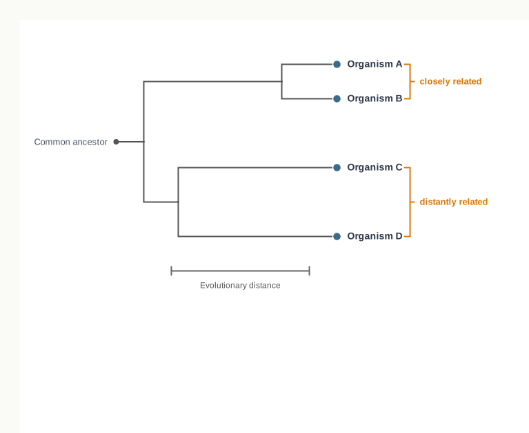
Fig. 9.11 – A simple phylogenetic tree (cladogram).

There are different methods for calculating evolutionary distances, and these are used by tools for phylogenetic analysis such as PHYLIP and PAUP. Because the methods differ, two trees built from the same sequences by different methods may not agree perfectly — which is why a published tree always names the method used to construct it.

The full downstream journey, from an assembled genome to a statement about function and ancestry, is summarised in Fig. 9.12.

Fig. 9.12

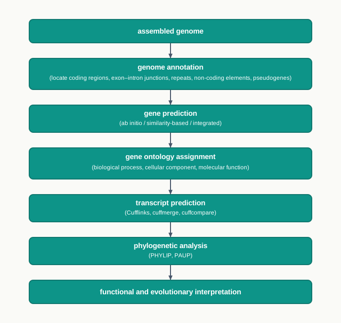
Fig. 9.12 – Downstream analysis of an assembled genome.

Try Yourself

A laboratory has sequenced an insect whose genome has never been studied before. Using Fig. 9.10 and Fig. 9.12, write down, in order, the steps they must follow from the raw FASTQ file to a phylogenetic tree placing their insect among related species. At each step, name one tool from Tables 9.5 and 9.6 or from Section 9.4.4 that they could use.

9.5 Role of Artificial Intelligence (AI) In Future

We are moving into an era in which the prospect of Artificial Intelligence (AI) is beginning to take hold. This section looks at what that means for a biologist, and it is worth reading with a cool head — both the enthusiasm and the caution in it are deliberate.

Machine learning, which was named in Section 9.1 as one of the computational concepts a modern biologist needs, is the branch of AI that matters most here. Rather than being given a fixed set of rules by a programmer, a machine learning system is shown a large number of examples and works out the pattern for itself.

Definition

Machine learning is an approach in which a computer program learns to recognise patterns from a large number of examples, instead of following rules written out in advance by a programmer.

What AI Has Already Achieved

Real Incident / Discovery

The first convincing public demonstrations of modern AI came not from a laboratory but from a games table. AlphaGo, built by a research team at DeepMind, defeated the leading professional player Lee Sedol at the ancient board game Go in 2016 — a result most experts had expected to be a decade away, because the number of possible positions in Go is far too large to work through by brute force. Not long after, a bot named Libratus, developed at Carnegie Mellon University, defeated top professional players at poker. Poker was in some ways the harder problem, because a poker player cannot see the opponent’s cards and must reason under uncertainty and deception — much closer to the conditions of real scientific data than a board game is.

These bots, Libratus and AlphaGo, have therefore already conquered real-life experts in games such as Poker and Go. The significance for biology is not that computers can play games. It is that a machine can now find reliable patterns in situations too complex for a human to reason through step by step — which is a fair description of a genome.

AI in Healthcare and Farming

Machine learning is also starting to make its presence felt in improving farming and in broadening healthcare options.

In healthcare, AI-based tools are used in the USA to diagnose eye diseases, working from thousands of stored images of the eye. The principle is the one described above: the system is shown a very large number of images in which the diagnosis is already known, learns what a diseased retina looks like, and then applies that learning to a new patient’s image.

It is quite possible that we will soon have computers reading X-rays and pathology slides routinely in hospitals, aiding radiologists and pathologists in diagnosing human diseases correctly and quickly. Notice the word aiding. The realistic picture is not a computer replacing a doctor, but a computer flagging what deserves a specialist’s attention first.

AI also holds significant promise for helping our farmers to improve their yield and to decide on which crops to grow. Soil data, weather records, satellite images of a field and past yield figures are exactly the kind of large, mixed, pattern-rich data on which machine learning performs well.

Bioethics

Letting an AI system read medical images An AI system that reads X-rays and pathology slides could bring expert-level screening to hospitals that have no specialist available, and could do it in seconds — a serious benefit in a country where radiologists and pathologists are unevenly distributed. Against that stand several real concerns. Such a system learns from the images it was trained on, so if those images came mostly from one population, its performance on a different population is unknown. Responsibility is also unclear: if a missed diagnosis follows an AI report, it is not obvious who is accountable. And the reasoning inside many machine learning models cannot be inspected the way a doctor’s reasoning can be questioned. The safeguards generally applied are that such tools are approved as medical devices by a regulatory authority before clinical use, that they are validated on local patient data rather than assumed to transfer, and that the AI output is treated as an aid to a qualified professional who makes and signs the final diagnosis — never as the diagnosis itself.

AI Already Inside Bioinformatics Tools

This is not only a future prospect. Many existing bioinformatics tools are already using machine learning algorithms for calling genomic variants and for assessing their significance levels.

Calling a variant means deciding, from the aligned sequencing reads described in Section 9.4, whether a difference from the reference genome at a given position is a genuine variant in that individual or merely a sequencing error. That decision is a judgement made under uncertainty, based on many pieces of evidence at once, which is precisely the kind of problem machine learning handles well.

Technique

Machine learning–based variant calling Principle: A genuine variant and a sequencing error leave different patterns of evidence in the aligned reads — the number of reads supporting the change, their quality scores, their positions within the reads — and a model trained on positions whose true status is already known can learn to tell the two apart. Steps: Align reads to the reference genome → at each position where reads differ from the reference, collect the supporting evidence → pass this evidence to a model trained on known true variants and known errors → the model reports a variant call with a confidence score → assess the significance of the called variant. Used for: Producing a reliable list of an individual’s genomic variants from raw sequencing data — the step on which clinical genome interpretation depends.

Fig. 9.13

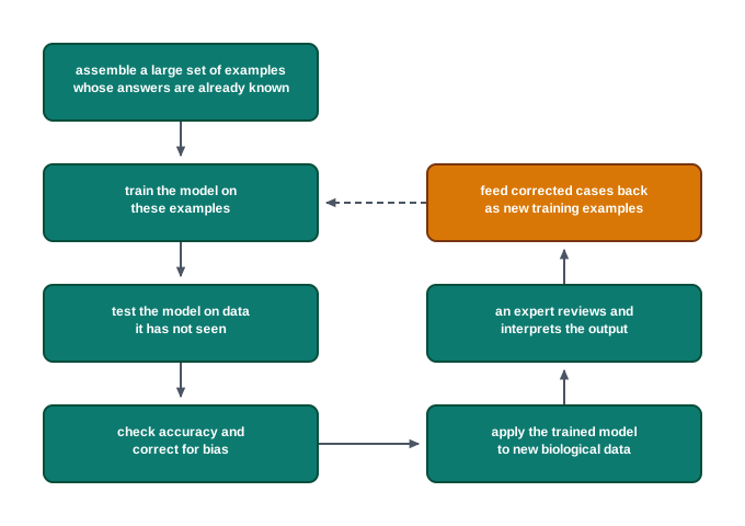
Fig. 9.13 – How a machine learning tool is built and used in bioinformatics.

The Honest Limits

Here the chapter becomes deliberately cautious, and the comparison it chooses is a familiar one. Personal assistants such as Siri from Apple or Alexa from Amazon are not perfect and cannot do everything, even after years of development on far simpler problems than biology. In the same way, a successful intersection between AI and bioinformatics will require time and multi-disciplinary effort before it yields reliable results.

Such a junction demands that sufficient intelligence be built into the tools, so that they can genuinely interpret data and generate hypotheses — not merely sort it. Interpretation and hypothesis generation are the two hardest things a biologist does, and they are the two things a tool must eventually manage if it is to be more than a fast calculator.

There is also a gap that is widening rather than closing. The competency of the tools being developed for analysis is still not at par with the fast pace at which the data is being produced. Data generation has become cheap and quick; making sense of that data has not.

Exam Corner

Q. If AI tools are already calling variants, why can they not simply be trusted to interpret the whole genome?

A. Because calling a variant and understanding what it means are different problems. Calling a variant is a well-defined pattern-recognition task with a clear right answer, which is what machine learning does well. Interpreting a genome requires asking whether a finding makes biological sense, connecting it to what is known about the organism, and framing the next question — the biological acumen that Section 9.1 warned could never be replaced by a statistical or computational method.

Curiosity Corner

Q5. Can a machine that learns on its own take over the job of interpreting biological data?

A. Not on its own, and not yet. Machine learning is already doing real work inside bioinformatics — calling genomic variants, assessing their significance, diagnosing eye disease from stored images — and it will do more. But the tools are still not competent enough to keep pace with the data being produced, and interpretation and hypothesis generation remain human tasks. The realistic future is collaboration, not replacement.

The Way Forward

The chapter ends on the point it has been building towards from its first page. A collaboration among researchers working in biology, computer science, bioinformatics, statistics and artificial intelligence will lead to successful tools for biological data analysis in the future.

That single sentence is a fair summary of bioinformatics itself: no one discipline can solve these problems alone, which is exactly why the field exists.

How This Section Is Tested

Questions on this section usually take one of two shapes. Either they ask you to name a concrete application of AI in healthcare or agriculture and explain the principle behind it, or they present an assertion–reason item in which the assertion overstates what AI can do — for instance, that AI tools can replace biologists in interpreting data — and the reason states something true about machine learning. Read such items carefully: a true reason does not automatically make an overstated assertion true.

Try Yourself

Write down two tasks in this chapter that you would confidently hand over to a machine learning tool, and two that you would insist on keeping with a human biologist. Give one line of justification for each of the four.

9.6 Summary

Bioinformatics is an interdisciplinary field that uses computational and statistical techniques to analyse and interpret biological data. It covers the storing, retrieving and analysing of biological information, usually with computer-based tools.
The outcome of every biological experiment is data. Because modern instruments produce data in enormous volumes, a biologist can no longer manage results with a notebook and a spreadsheet alone.
Modern biologists therefore need advanced computational and statistical tools to manage, analyse and interpret large datasets. Key statistical methods such as correlation and regression play an essential role in drawing meaningful conclusions from experimental data.
Statistics can only aid interpretation; it cannot replace asking the right biological question. Choosing the wrong test, or applying a model whose assumptions do not fit the data, produces confident but false results.
The historical perspective traces bioinformatics from early structural bioinformatics, which focused on protein structures, to today’s genome-wide assays driven by advances in sequencing technology. Milestones include the creation of GenBank in 1982 and the launch of the Human Genome Project in 1991, both of which significantly advanced the field.
Various biological databases, such as nucleotide and protein databases, make it possible to organise vast amounts of biological data. One of the major resources, the National Center for Biotechnology Information (NCBI), is central to representing and assessing sequence data in common data formats such as FASTA.
A good biological database is easy to use, well documented, error-free, cross-referenced, and continually updated as its primary sources change. Databases may be relational, queried through SQL, or non-relational (NoSQL) for large, distributed and unstructured data.
Genome informatics is the application of bioinformatics tools to the outputs of genome-wide assays, so that the data can be interpreted and linked to function. Such tools and workflows are vital for analysing the sequence data generated by high-throughput sequencing technologies.
Sequenced reads are handled in one of two ways: they are aligned to a reference genome where one exists, or assembled de novo into a draft genome where none exists. In both cases the raw data is first checked and trimmed for quality.
Downstream analysis turns sequence into biology through genome annotation, gene prediction, gene ontology assignment, transcript prediction and phylogenetic analysis.
The potential applications of artificial intelligence (AI) in bioinformatics are discussed in the context of games and sports, healthcare and agriculture. AI tools are increasingly employed for tasks such as diagnosing diseases and improving crop yields.
The competency of analysis tools has not yet caught up with the speed at which data is produced. Continuing multidisciplinary collaboration between biologists, computer scientists, statisticians and AI researchers is essential for developing intelligent bioinformatics tools.

Fig. 9.14

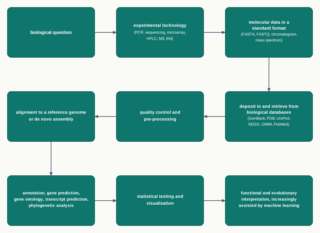
Fig. 9.14 – The chapter in one sequence.

9.7 Key Terms

Data — The set of readings, counts, images, sequences or measurements that a biological experiment actually produces, before any conclusion is drawn from it.
Quantitative analysis — Numerical analysis applied to large volumes of data in order to interpret them and generate biological meaning.
Null hypothesis — A statement that there is no relationship between two measured phenomena.
Statistical significance — The property of a result that is very unlikely to have occurred by chance.
p-value — The probability of finding the observed results when the null hypothesis of a study question is true.
t-test — An analysis of two population means through the use of statistical examination.
Multivariate analysis — A set of techniques used for the analysis of data containing more than one variable.
Regression analysis — A technique to investigate the relationship between a dependent and an independent variable.
Multiple testing correction — A statistical test that corrects for multiple tests, keeping the overall error rate less than or equal to the user-specified P-value cutoff.
Analysis of Variance (ANOVA) — A collection of statistical models used to analyse the differences among group means in a sample.
Correlation — A measure of how closely two measured variables are connected to each other.
Regression — A statistical relationship defined between two or more variables, in which a change in one variable is associated with a change in another.
R²-value — The output of a linear regression analysis, showing how close the data are to the fitted regression line, ranging from 0 for no correlation to 1 for perfect correlation.
Biological replicate — An independent biological sample included in an experiment to test whether a result holds across individuals.
Technical replicate — A repeated measurement of the same sample, included to test the reliability of the measurement itself.
Law of large numbers — The statistical principle underlying the fact that random sampling from a large number reduces the chance of obtaining biased results.
Statistical power — The ability of a test to detect a real effect if one exists, which must be considered for positive as well as negative results.
MATLAB — A commercial built-in framework used by biologists for higher levels of computing, analysis and visualisation.
R — An open-source software environment for statistical computing and for generating graphics.
Bioinformatics — The interdisciplinary field that applies computational, mathematical, statistical and sometimes engineering approaches to the storage, retrieval, analysis and interpretation of biological data.
Data mining — The systematic searching of large stored datasets for patterns, used in bioinformatics to make new findings and generate new hypotheses.
Next-generation sequencing — A high-throughput technology used to sequence genes, genomes and RNA.
DNA microarray — A high-throughput technology in which labelled sample nucleic acid binds to known probes fixed at defined positions on a chip, allowing many sequences to be assayed at once.
National Center for Biotechnology Information (NCBI) — A resource in the USA created for bioinformatics tools and services, housing nucleotide, protein and bibliographic databases.
GenBank — A widely used database, launched in 1982, that stores annotated, publicly available DNA sequences.
Protein Data Bank (PDB) — A collection of the 3D structures of proteins, nucleic acids and complex assemblies.
Structural bioinformatics — The branch of bioinformatics dealing with three-dimensional structures of macromolecules, which pre-dates informatics based on genome-wide assays.
In silico — Performed on a computer, as opposed to in vivo in a living organism or in vitro in glassware.
Frameshift error — An in silico translation error in which a wrongly recorded base shifts the reading frame, so that every codon after that point is read incorrectly.
Polymerase Chain Reaction (PCR) — A technology used to amplify a region of DNA of interest.
Real-Time PCR / quantitative PCR (qPCR) — A technology used to detect RNA expression by measuring product as the reaction proceeds.
Gel electrophoresis — A technique that separates DNA, RNA and protein fragments on the basis of their size and charge.
High-performance Liquid Chromatography (HPLC) — A technique used for the separation, identification and quantification of metabolites, producing a chromatogram.
Mass spectrometry (MS) — A technique used for fragmentation, measurement of isotopic composition and mass determination, producing a mass spectrum.
Electron microscope (EM) — An instrument used for structure and sequence determination of DNA, RNA or protein.
Loss-of-function assay — A test in which a gene is disabled so that the resulting change in the organism reveals the gene’s normal function.
Gain-of-function assay — A test in which a gene is added or over-expressed so that the resulting change reveals its function.
Biological database — A repository containing an organised, structured and searchable collection of biological data, linked back to its original creators or reference.
Single nucleotide polymorphism (SNP) — A position in the genome at which a single base commonly differs between individuals of a population.
Database management system (DBMS) — The software system used to manipulate, retrieve and manage the data held in a database.
Structured query language (SQL) — The standard application program interface used to query a relational database.
Non-relational or NoSQL database — A database that does not follow the order of a relational database, used for large sets of distributed and unstructured data.
UniProt — A database holding a collection of protein sequences and their functions.
PubMed — A database holding a collection of biomedical literature.
KEGG — A collection of biological pathways, diseases, drugs and chemical substances, also used as a pathway visualisation tool.
OMIM — A catalogue of human genes and genetic disorders.
Data visualisation — The application of graphics and data representation to biological data such as sequences, genomes, alignments, phylogenies, structures and microscopy images.
UCSC Genome browser — An online interactive website used to visualise macro- and micro-level genome information for vertebrate and invertebrate species.
CIRCOS — A tool used to visualise data in a circular layout.
Integrative Genomics Viewer (IGV) — A tool for the interactive exploration of large, integrated genomic datasets.
Genome — The complete set of DNA of an organism, including its genes and the intergenic regions.
Genomics — The field of science dealing with the structure, function, evolution, mapping and modification of genomes.
Genome informatics — The application of bioinformatics tools to process the outputs of genome-wide assays, so that the data can be interpreted and linked to function.
Omics fields — The group of fields, including genomics, transcriptomics, proteomics and metabolomics, that each study a whole class of molecules at once.
High-throughput — Describing a process or instrument that produces a significant amount of data in a single run.
Human Genome Project — The initiative begun in the early 1990s to sequence the complete nucleotide content of human cells, whose first complete draft was published in 2001.
Whole-genome shotgun sequencing — A method in which randomly cut genomic DNA is sequenced and the fragments are then reassembled computationally using their overlaps.
Euchromatin — The loosely packed, gene-rich chromosomal region that makes up most of the sequenced part of the human genome.
Heterochromatin — The tightly packed, repeat-rich chromosomal region, mainly around centromeres and telomeres, that remains difficult to sequence and assemble.
FASTQ — A text-based format that stores sequence information together with its corresponding quality scores, typically using four lines per sequence.
FASTA — A text-based format for representing sequence information in single-letter codes, whose first line begins with a > symbol.
Read — One continuous stretch of sequence reported by a sequencing instrument, either short (about 100–150 nucleotides) or long (a few kilobases).
De novo assembly — The workflow in which reads are pieced together using their overlaps and insert size to build a draft genome, without any reference sequence.
Contig — A contiguous stretch of sequence formed by assembling overlapping reads.
Insert size — The distance between paired-end reads, used along with overlaps during assembly.
FastQC — A quality control tool used to check high-throughput sequence data.
Trimmomatic — A tool used for quality and adaptor trimming of raw sequencing data.
BLAST (Basic Local Alignment Search Tool) — A tool that searches a nucleotide or protein query sequence against a non-redundant sequence database.
BLAT — A BLAST-like alignment tool that stores the genome index in memory and is designed to quickly find highly similar sequences (>95%) of at least 40 nucleotides.
Multiple sequence alignment — The alignment of several sequences together, carried out by programs such as CLUSTAL, MUSCLE and T-Coffee.
SAM and BAM — Sequence Alignment/Mapping format and its compact Binary Alignment/Mapping equivalent, interconverted using SAM tools.
Genome annotation — The process of identifying and classifying all the features present in a genome.
Transposon — A category of repeat element that forms the most significant chunk of the repeats in a genome.
Satellite — A category of repetitive DNA recognised during genome annotation.
Low complexity region — A category of repeat element consisting of simple, low-diversity sequence.
Gene prediction — The identification of all the coding sequences in a genome, using ab initio, similarity-based or integrated approaches.
Ab initio approach — A gene prediction strategy that works from the statistical features of the sequence itself rather than from similarity to known genes.
Gene Ontology — A system describing gene products in terms of their associated biological processes, cellular components and molecular functions, so that functions are represented without ambiguity.
Transcript prediction — The prediction of coding and non-coding transcripts, carried out by tools such as Cufflinks, cuffmerge and cuffcompare.
Phylogenetic analysis — Analysis carried out to determine the evolutionary relationship of an organism with others, using tools such as PHYLIP and PAUP.
Cladogram or phylogenetic tree — A diagram expressing evolutionary relationships, in which distance indicates how closely organisms are related on an evolutionary scale.
Artificial Intelligence (AI) — The use of computers to perform tasks that would normally be said to require human judgement.
Machine learning — An approach in which a program learns patterns from large numbers of examples rather than following rules written in advance.
Variant calling — Deciding, from sequencing data, whether an apparent difference from the reference genome is a real variant or an error, a task increasingly performed using machine learning algorithms.

9.8 Points to Ponder

The chapter states that mathematical and statistical concepts can only aid a biologist and are not a replacement for asking the right questions or for biological acumen. What would a perfectly executed statistical analysis of a badly framed biological question actually look like — and how would a reader spot it?
A regression on ten patients gave \(R^2 = 0.8567\), and the null hypothesis was rejected. Would you be equally confident if the same \(R^2\) had come from only three patients? Think about what the number does, and does not, tell you about sample size.
The P value cutoff of 0.05 is a convention, not a law of nature, and the chapter says it has allowed too many false positives into the scientific literature. If a threshold that has been used for decades is now known to mislead, what should the scientific community do about the results already published under it?
Consider the advice that with small sample sizes it is better to show all the independent data points than to present an average and a standard deviation. What does this suggest about the relationship between honesty and simplicity in a scientific figure?
Bioinformatics was practised long before the word existed, and the term itself entered the literature only in 1991. Does naming a field change the science being done in it, or only how that science is organised, funded and taught?
Structural bioinformatics came before genome informatics, yet most students meet genome data first. What might a biologist miss by learning the sequence side of the subject without the structural side?
Database entries are continually corrected for frameshift errors, annotation errors, assembly errors and even spelling mistakes. If the contents of a database can change after your analysis is published, what does reproducibility mean in bioinformatics?
A good biological database is described as one that lacks errors in its underlying data. Given that databases accept deposits from thousands of laboratories, is a completely error-free biological database a realistic goal or a useful ideal? What follows from your answer?
Human genomic data is most useful when it is shared widely, and most dangerous to privacy for exactly the same reason. Where would you draw the line between what should be openly available and what should be released only under controlled access — and who should be allowed to draw it?
The human genome was announced in 2003, yet the heterochromatic regions remain poorly represented. Is it accurate to describe such a sequence as a “complete genome”? Consider what is gained and lost by the way scientific milestones are announced to the public.
Assembly software can either leave a gap where a repeat cannot be placed unambiguously, or guess a position and move on. Which choice serves science better, and why might the honest choice be the harder one to defend to a funding agency?
FASTQ stores one quality score for every single base. Suggest what would be lost if the format instead stored a single average quality score for each read, and what would be gained.
The chapter notes that the competency of analysis tools has not kept pace with the speed at which data is produced. What are the consequences of a science that can generate far more data than it can interpret? Is more data always progress?
An AI system can now diagnose eye disease from stored images, but the chapter insists that interpretation and hypothesis generation remain human tasks. What exactly is it that a biologist does which a pattern-recognition system, however powerful, cannot yet do?
Bioinformatics exists because no single discipline could solve these problems alone. What are the practical difficulties — of language, training and habit — when a biologist, a statistician and a computer scientist sit down to work on the same data set?

9.9 NCERT Questions

Name the two modalities of analysis following sequencing.
Name any three major types of variants.
What are disease-specific variants termed?
1. somatic
2. germline
Which is the preferred tool for transcriptome assembly, in the de novo and genome-guided modalities?
1. Tophat2
2. Trinity
What is the difference between BLAT and BLAST?
What came first? Structural Bioinformatics or Genome informatics?
Name any two of the major classes of biological macromolecules.
DNA sequences can be represented by which of the following data format?
1. FASTQ
2. FASTA
3. AB1
4. All of the above
Can a phylogeny be produced directly from a multi-fasta file? Justify your answer.
Which tool can help you visualise variants in a circular manner?
1. UCSC Genome Browser
2. CIRCOS
3. IGV
Why do we need to sequence nucleic acids? What can one gain by understanding the sequence of a nucleic acid?

9.10 Objective Questions

The outcome of any biological experiment is:
1. a conclusion
2. data
3. a hypothesis
4. a statistical test
A statement that there is no relationship between two measured phenomena is called the:
1. alternative hypothesis
2. null hypothesis
3. p-value
4. regression line
The \(R^2\) value obtained from a linear regression analysis can range between:
1. \(-1\) and \(+1\)
2. \(0\) and \(100\)
3. \(0\) and \(1\)
4. \(0.05\) and \(0.95\)
A P value cutoff conventionally considered significant is:
1. 0.5
2. 0.05
3. 5.0
4. 0.95
A collection of statistical models used to analyse the differences among group means in a sample is:
1. t-test
2. multivariate analysis
3. ANOVA
4. multiple testing correction
Which of the following quantifies how two variables are connected, without treating one as dependent on the other?
1. Regression
2. Correlation
3. Statistical power
4. Multiple testing correction
Which of the following is an open-source framework used by biologists for computing, analysis and visualisation?
1. MATLAB
2. SPSS
3. R
4. SAS
Bioinformatics deals with the storage, retrieval, analysis and interpretation of biological data. It is best described as:
1. a branch of computer science
2. a branch of statistics
3. an interdisciplinary field
4. a laboratory technique
GenBank, the database storing all publicly available DNA sequences, was launched in:
1. 1965
2. 1982
3. 1991
4. 2001
The term ‘bioinformatics’ started appearing in the scientific literature in:
1. 1982
2. 1991
3. 2001
4. 2003
Which technology from Table 9.2 is used for the separation, identification and quantification of metabolites?
1. Mass spectrometry
2. Gel electrophoresis
3. HPLC
4. qPCR
Gel electrophoresis separates fragments on the basis of their:
1. size and charge only
2. mass and isotopic composition
3. sequence and quality score
4. solubility and boiling point
The standard application program interface for a relational database is:
1. DBMS
2. SQL
3. NoSQL
4. BLAST
A database used for large sets of distributed and unstructured data is described as:
1. relational
2. non-relational (NoSQL)
3. bibliographic
4. secondary
A catalogue of human genes and genetic disorders is maintained by:
1. UniProt
2. PDB
3. OMIM
4. PubMed
Three-dimensional structures of proteins, nucleic acids and complex assemblies are collected in:
1. GenBank
2. PDB
3. KEGG
4. PubMed
The genome of an organism consists of:
1. only its protein-coding genes
2. only its exons
3. its complete DNA, including genes and intergenic regions
4. its complete set of transcripts
The term ‘high-throughput’ refers to a process that:
1. is highly accurate
2. produces a significant amount of data
3. requires no computational analysis
4. works only on protein samples
Celera Genomics sequenced randomly cut human DNA using a technique called:
1. clone-by-clone sequencing
2. whole-genome shotgun sequencing
3. capillary gel electrophoresis
4. re-sequencing
The regions of the human genome that remain poorly sequenced are mainly:
1. euchromatic and gene-rich
2. heterochromatic, repetitive, near centromeres and telomeres
3. exonic regions of housekeeping genes
4. the intergenic regions of chromosome 1 only
In a FASTQ file, the line that begins with the ‘@’ character is:
1. line 1
2. line 2
3. line 3
4. line 4
In a FASTQ record, the number of symbols in line 4 must be:
1. half the number of letters in line 2
2. equal to the number of letters in line 2
3. fixed at 150
4. independent of line 2
In the quality line of a FASTQ file, the character representing the lowest quality is:
1. >
2. +
3. !
4. ~
Short sequence reads produced by high-throughput sequencing instruments are usually about:
1. 10–15 nucleotides
2. 100–150 nucleotides
3. 1000–1500 nucleotides
4. a few kilobases
Trimmomatic is used for:
1. assembling reads into contigs
2. quality and adaptor trimming
3. converting SAM to BAM
4. predicting genes
BLAT is designed to quickly find highly similar sequences with an identity greater than:
1. 40%
2. 75%
3. 95%
4. 99.9%
Repeats in a genome are classified into three major categories. The one forming the most significant chunk is:
1. satellites
2. low complexity regions
3. transposons
4. pseudogenes
The Gene Ontology describes gene products in terms of biological processes, cellular components and:
1. evolutionary distances
2. molecular functions
3. quality scores
4. insert sizes
Cufflinks, cuffmerge and cuffcompare belong to a suite used for:
1. quality control
2. transcript identification
3. phylogenetic analysis
4. format conversion
PHYLIP and PAUP are tools used for:
1. genome assembly
2. gene ontology assignment
3. phylogenetic analysis
4. pathway visualisation
Assertion (A): A biologist today cannot manage experimental results using only a notebook and a spreadsheet. Reason (R): High-throughput sequencers, imaging systems and analytical instruments generate data in volumes that require computational and statistical tools for interpretation.
Assertion (A): A high \(R^2\) value alone proves that a change in one variable causes a change in the other. Reason (R): The \(R^2\) value measures how close the data points lie to the fitted regression line.
Assertion (A): Applying a Gaussian distribution to a nonlinear dynamical system is a common statistical abuse. Reason (R): Every statistical model carries assumptions about how the data behave, and violating them can produce false positives.
Assertion (A): Structural bioinformatics preceded informatics based on high-throughput genome-wide assays. Reason (R): Studies of three-dimensional protein structures using NMR spectroscopy and X-ray crystallography pre-date the -ome informatics fields.
Assertion (A): Biological information must be encoded in a machine-readable format before it can be searched. Reason (R): Nucleotide sequences, genes and protein structures are tiny and cannot be searched physically the way books on a library shelf can.
Assertion (A): A good biological database is cross-referenced and continually updated. Reason (R): Biological data is dynamic, and entries such as exon–intron boundaries and annotations are revised as understanding improves.
Assertion (A): The human genome sequence available today still contains gaps. Reason (R): Heterochromatic regions are largely repetitive, difficult to assay with current sequencing technology, and difficult to assemble unambiguously to a single chromosomal location.
Assertion (A): De novo assembly is chosen when no reference genome is available for the organism being studied. Reason (R): De novo assembly pieces reads together using their overlaps and the insert size between paired-end reads.
Assertion (A): Sequencing data must be quality-checked and trimmed before assembly or alignment is attempted. Reason (R): Every downstream step treats its input as true, so poor-quality bases and adaptor sequences would be carried silently into the final result.
Assertion (A): Machine learning tools can already call genomic variants and assess their significance. Reason (R): The competency of analysis tools has now caught up with the pace at which biological data is produced.

9.11 Check Your Concepts

Why is it said that mathematical and statistical concepts can only aid a biologist, and cannot replace asking the right question? Explain with reference to what a statistical test actually does.
A student plots blood pressure against heart rate for ten patients and says, “I can see they are related.” What is wrong with stopping at this point, and what must the student do next to make a defensible claim?
Distinguish between correlation and regression under the following heads: what each measures, how the variables are treated, and the typical output of each.
An analysis returns \(R^2 = 0.12\). State what this tells you about the scatter of the data around the fitted line, and explain why failing to reject the null hypothesis is not the same as proving that no relationship exists.
Why must a biologist settle questions of sample size and number of replicates before performing an experiment rather than after the data are collected?
Distinguish between a biological replicate and a technical replicate, and give one situation in which having many technical replicates but only one biological replicate would mislead a researcher.
Explain why random sampling from a large number reduces the chance of obtaining biased results. Relate your answer to the law of large numbers.
Why does running many statistical tests at once make multiple testing correction necessary? What would happen if a researcher reported every test that crossed the 0.05 threshold without applying any correction?
The chapter advises that with small sample sizes it is better to show all independent data points than an average with a standard deviation. Explain the reasoning behind this advice.
What is meant by statistical power? Explain why it should be considered when a result is positive, and not only when it is negative.
Bioinformatics is described as interdisciplinary. Name the disciplines that intersect in it and state, for each one, what it contributes to the analysis of biological data.
Arrange the following in the correct order as shown in Fig. 9.4, and write one line explaining what happens at each stage: analytical and statistical workflows; biomolecules; functional interpretation; molecular data; experimental technology.
Match each technology in Column I with the biomolecule it assays in Column II and its purpose in Column III.

Column I (Technology)	Column II (Biomolecule)	Column III (Purpose)
a. qPCR	i. Metabolites	p. Amplify a region of interest
b. HPLC	ii. DNA	q. Detect RNA expression
c. PCR	iii. DNA, RNA and proteins	r. Separation, identification and quantification
d. Gel electrophoresis	iv. RNA	s. Separation of fragments by size and charge

Why is a standard data format such as FASTA or FASTQ necessary in bioinformatics? Describe what would go wrong if every sequencing instrument wrote its output in its own private format.
Explain why a database entry that carries no link back to its original creator or reference is of limited scientific value.
A library and a sequence database both solve a search problem, but only one of them can be searched physically. Explain this difference and state what it forces bioinformatics to do with biological information.
List any five characteristics of a good biological database, and explain why “continually updates information as and when the primary source is updated” is essential rather than merely desirable.
Compare relational and non-relational (NoSQL) databases under the heads: organisation of data, kind of data suited to each, and standard query interface.
For each of the following, name the most appropriate database and justify your choice in one line: (i) the published literature on a disease, (ii) the atomic structure of an enzyme, (iii) the annotated DNA sequence of a gene, (iv) the metabolic pathway a protein belongs to.
Why is it useful for a database to record the frequency of an SNP across different populations, rather than merely recording that the SNP exists?
Two researchers want to display genomic data. One chooses the UCSC Genome browser and the other chooses CIRCOS. Explain what each is likely to be trying to show, and why the layout matters.
Define a genome. Explain why it would be incorrect to describe a genome simply as “the set of all genes of an organism”.
Distinguish between genomics and genome informatics, and state how the two depend on each other.
The publicly funded human genome effort and Celera Genomics both used Sanger’s method with modifications, yet followed different strategies. Compare the two strategies and explain why the shotgun approach placed a far greater burden on computation.
“The human genome was completed in 2003.” Evaluate this statement. Your answer should refer to euchromatin, heterochromatin, and the problem of assembling repetitive DNA.
Draw a labelled representation of a FASTQ record showing all four lines. Label the character that begins line 1, the character that begins line 3, and state the rule connecting the lengths of lines 2 and 4.
A FASTA header reads >K02382.1 Human growth hormone synthetic gene, complete cds. Identify the accession number, the identifier, the source and the type of sequence, and state the purpose of the > symbol.
Compare FASTA and FASTQ formats. Explain why a high-throughput sequencer outputs FASTQ rather than FASTA, and why a database entry may be perfectly adequate in FASTA.
Why does a sequencer report a quality score for every individual base rather than one score per read? Relate your answer to the purpose of trimming.
Name the two modalities of analysis that follow sequencing, and explain what determines which one a laboratory must use.
A student proposes the following protocol for a newly sequenced bacterium: (1) obtain reads, (2) assemble reads into contigs, (3) run FastQC, (4) predict genes, (5) build a phylogenetic tree. Identify the error in the order of the steps, correct it, and explain what would go wrong if the protocol were followed as written.
Explain the roles of read overlap and insert size in de novo assembly. Why is a contig described as “contiguous”, and why does an assembly usually consist of many contigs rather than one?
Study Fig. 9.9. Describe what is happening at each of the three stages shown, and explain why the middle stage is the one that makes assembly possible.
Compare BLAST and BLAT under the heads: where the index is stored, the degree of similarity each is designed to detect, minimum sequence length, and relative speed. State one situation in which BLAST would be preferred despite being slower.
SAM tools convert SAM files to BAM files. Explain what is gained by this conversion, given that the biological information in the two files is identical.
What is genome annotation? List the features that are identified during annotation of an assembled genome.
Repeats are sometimes dismissed as unimportant. Using the chapter’s account, argue against this view. Name the three major categories of repeats and state which forms the largest share.
Compare the ab initio and similarity-based approaches to gene prediction. Explain why the integrated model is generally considered superior to either one alone.
Why is the Gene Ontology necessary? Explain the problem it solves and name the three categories in which it describes gene products.
What does a cladogram represent, and what does the distance between two organisms on it indicate? Explain why two trees built from the same sequences by different tools may not agree.
Explain the principle by which an AI-based tool learns to diagnose an eye disease from stored images. What limitation follows if all the training images came from a single population?
Machine learning already performs variant calling, yet the chapter insists that interpretation remains a human task. Distinguish between these two activities and explain why one is far better suited to a machine than the other.
The chapter states that the competency of analysis tools has not kept pace with the rate at which data is produced. Explain the practical consequences of this gap for a research laboratory.

9.12 Case-Based Questions

A resident doctor in a cardiology ward records the heart rate and systolic blood pressure of ten admitted patients. Plotting one against the other, she feels that the two rise together, and she writes in her report that a raised heart rate causes a rise in blood pressure. Her supervisor asks her to fit a regression line before writing anything further. She does so and obtains \(R^2 = 0.8567\).
1. Why was the supervisor unwilling to accept the conclusion drawn from a visual impression of the plot?
2. State the null hypothesis for this study, and explain what the obtained \(R^2\) value allows her to do with it.
3. The resident had written that a raised heart rate causes a rise in blood pressure. Is this claim justified by her analysis? Give a reason.
4. If she had recorded only three patients and obtained the same \(R^2\) value, would your answer to sub-question 2 change? Explain.
A laboratory receives its first batch of data from a next-generation sequencing run. The file is in FASTQ format and contains 40 million reads, each of 150 bases. A junior researcher, eager to save time, loads the file straight into the assembly software. The resulting assembly contains several short stretches of sequence that do not match any known organism, and the ends of many contigs are unreliable.
1. Name the two pre-processing tools the researcher should have used, and state the function of each.
2. Explain how the short unmatched stretches of sequence could have entered the assembly.
3. In a FASTQ record, which line reports the reliability of each base, and how many symbols must that line contain for one of these reads?
4. Why does sequencing quality typically fall towards the end of a read, and how does this explain the unreliable contig ends?
A research group sequences the genome of an insect that has never been studied before. There is no reference genome available for this species or for any close relative. After assembly, they find that the regions around the centromeres are represented only by gaps in their draft sequence.
1. Which of the two modalities of analysis following sequencing must this group use, and why is the other one unavailable to them?
2. Explain, in terms of overlaps and insert size, how their draft genome was built.
3. Give one experimental reason and one computational reason for the gaps near the centromeres.
4. A colleague suggests filling the gaps by placing each repeat in the first position where it fits. Evaluate this suggestion.
A Class 12 student is asked to prepare a report on a single human gene. She begins with the gene’s nucleotide sequence, then wants the sequence and function of the protein it encodes, then the three-dimensional structure of that protein, then the metabolic pathway it belongs to, then any genetic disorder associated with it, and finally the published research papers on it.
1. Name the database she should consult at each of the six stages.
2. Which characteristic of a good biological database allows her to move from one of these resources to the next without retyping any sequence?
3. She notices that the annotation of the gene has changed since a paper published three years ago. Explain why database entries are revised in this way.
4. Explain why she cannot search for this gene the way a librarian searches a shelf for a book.
A national programme proposes to sequence the genomes of one lakh volunteers in order to build a database of variant frequencies for the country’s populations. The programme plans to release all the data openly on the internet so that any researcher anywhere can use it. A committee is asked to review the proposal.
1. State two clear scientific benefits of making such data widely available.
2. State two concerns that the committee would be expected to raise about releasing individual-level human genomic data openly.
3. Genetic information affects people who never volunteered for the study. Explain how, and why this complicates the question of consent.
4. Describe the two-tier arrangement commonly used as a safeguard in such programmes.
After assembling a fungal genome, a team runs gene prediction software. Using a similarity-based approach alone, the software predicts 9,400 genes. When the team repeats the analysis using an integrated model, the number rises to 10,100. Several of the additional genes have no match in any existing database.
1. Explain the principle on which the similarity-based approach works, and name a program used for it.
2. Why did the similarity-based approach miss the additional genes?
3. Which approach, working within the integrated model, was able to detect them, and on what basis?
4. After prediction, the team must describe the functions of the gene products without ambiguity. Name the system they would use and its three descriptive categories.
A district hospital with no resident ophthalmologist installs an AI-based tool that screens retinal images for eye disease. The tool was trained on thousands of stored images collected in another country. In its first month, it correctly flags several patients who are then referred to a city hospital, but it also reports two cases that the visiting specialist finds to be normal.
1. Explain the principle by which such a tool arrives at a diagnosis.
2. State one clear benefit of installing this tool in a hospital of this kind.
3. The tool was trained on images from a different population. Explain why this is a legitimate concern, and what step should be taken before relying on it.
4. Should the tool’s report be treated as the final diagnosis? Justify your answer with reference to the safeguards described in this chapter.
Two students are given the same data set: a list of variants detected across all the chromosomes of a single patient, along with several rearrangements linking distant parts of the genome. Student A displays the data in the UCSC Genome browser. Student B displays the same data using CIRCOS. Their teacher tells them that both figures are correct, but only one of them answers the question that was asked.
1. Describe the layout each of the two tools uses to display genomic information.
2. The question asked was: “Which distant regions of this genome have become joined to one another?” Whose figure answers it better, and why?
3. Suggest a different question, answerable from the same data set, for which the other student’s figure would be the better choice.
4. Name one more visualisation tool from this chapter that could be used for interactive exploration of large, integrated genomic datasets.

9.13 Practice With Data

Use the heart rate and blood pressure readings of the ten patients given in Table 9.1.
1. Calculate the mean heart rate and the mean systolic blood pressure for the group.
2. Which patient shows the greatest departure from the general trend of the group? Identify the patient and state the reason for your choice.
3. The regression on this data gave \(R^2 = 0.8567\). State what this value means about how close the points lie to the fitted line.
Four separate studies fit linear regression lines to their data and report the following values: Study I, \(R^2 = 0.12\); Study II, \(R^2 = 0.49\); Study III, \(R^2 = 0.86\); Study IV, \(R^2 = 0.97\).
1. Arrange the four studies in increasing order of how closely their data fit the regression line.
2. Express each \(R^2\) value as a percentage.
3. In which study is the case for rejecting the null hypothesis weakest, and why?
A researcher performs three tests on the same data set and obtains P values of 0.048, 0.006 and 0.21.
1. Using the conventional cutoff, which of these results would be called statistically significant?
2. Which result lies closest to the cutoff, and why should the researcher be especially cautious about it?
3. The researcher has run several tests on one data set. Name the statistical adjustment that must now be applied, and state its purpose.
A large genome centre produces 24 TB of genome data per day.
1. Calculate the output for one week and for one year of 365 days, in TB.
2. Express the annual figure in petabytes, given that \(1 \text{ PB} = 1024 \text{ TB}\).
3. If one portable hard disk stores 2 TB, how many such disks would be filled by a single day’s output?
A sequencing run produces 40 million reads, each 150 nucleotides long.
1. Calculate the total number of bases generated in the run.
2. If these reads are used to sequence a genome of \(3.2 \times 10^{9}\) base pairs, calculate the coverage, using \[\text{Coverage} = \frac{\text{Number of reads} \times \text{Read length}}{\text{Genome size}}\]
3. State what your answer means in plain words about how many times, on average, each base of the genome was read.
A FASTQ record has 150 letters in line 2.
1. How many symbols must line 4 contain, and why?
2. After trimming, only the first 118 bases are retained. Calculate the percentage of the read that was discarded, correct to one decimal place.
3. If the same trimming is applied to all 40 million reads of the run, how many bases survive in total?
A quality control report on a sequencing run shows that 6.4 million of the 40 million reads fail the quality threshold and are removed, and that adaptor sequence is detected in a further 1.2 million reads.
1. Calculate the percentage of reads removed for poor quality.
2. Calculate the percentage of the original reads that carried adaptor sequence.
3. If the adaptor-containing reads are trimmed rather than discarded, how many reads remain available for assembly?
BLAT is designed to find highly similar sequences of more than 95% identity and of at least 40 nucleotides. Four query matches are obtained as follows:

Match	Length of match (nucleotides)	Identity (%)
I	62	98.4
II	35	99.1
III	120	91.0
IV	44	96.5

a. Which of these matches satisfy both of BLAT's design criteria?
b. For each match that fails, state which criterion it fails and by how much.
c. Suggest which tool would be more suitable for detecting match III, and give a reason.

An alignment file in SAM format occupies 96 GB. After conversion to BAM format, the same information occupies 24 GB.
1. Calculate the reduction in file size as a percentage of the original.
2. Express the size of the BAM file as a fraction of the SAM file, in its simplest form.
3. State one advantage and one disadvantage of storing the data in the binary form.
Sequenced reads of 150 nucleotides each are being assembled into a contig. Two reads overlap over 90 nucleotides.
1. Calculate the length of the contig formed by joining just these two reads.
2. A third read of the same length is then joined, overlapping the contig by 70 nucleotides. Calculate the new contig length.
3. Explain why the contig grows by less than 150 nucleotides each time a read is added.
A chromatogram from an HPLC run shows three peaks, at 17 minutes, 43 minutes and 66 minutes, with absorbance values at 254 nm of 11 AU, 22 AU and 13 AU respectively.
1. Which axis identifies the compound, and which axis reports how much of it is present?
2. Which of the three compounds is present in the greatest amount, and what is the ratio of the largest peak to the smallest?
3. A second run of the same sample gives peaks at the same three times but with all absorbance values halved. What has most likely changed between the two runs?
A biological database held 1.2 million sequence entries at the end of one year, and the number of entries doubled every year thereafter.
1. Calculate the number of entries at the end of the fourth year that follows.
2. Write a general expression for the number of entries \(N\) after \(n\) years, in terms of the starting number \(N_0\), and state what each symbol represents.
3. State what this pattern of growth explains about the need to store biological information in databases rather than in laboratory notebooks.