Chapter 12: Tools and Techniques
This chapter is long enough to split. This is the first part (Part A), ending just before Section 12.5. Reply to continue, and I will produce Part B and then automatically merge and renumber the complete, unbroken file.
In a quiet laboratory in Cambridge, England, a soft-spoken biochemist named Frederick Sanger spent decades doing something most scientists thought was impossible: reading the molecules of life letter by letter. In 1958 he received the Nobel Prize in Chemistry for working out the structure of the insulin molecule — the first time anyone had shown that a protein has one exact, fixed sequence of amino acids, and not a random arrangement. That single result changed how biologists thought about proteins forever.
But Sanger did not stop there. He turned to a far harder target: DNA. He wanted to read the order of the four bases along a DNA strand, and for that he needed a method that did not yet exist. He invented one, based on separating tiny DNA fragments on a gel and “reading off” their order. In 1977 he used it to sequence the genome of the bacteriophage ΦX174 — the first complete genome of any organism ever read. In 1980 he received a second Nobel Prize in Chemistry, shared with Paul Berg and Walter Gilbert, for this work on determining base sequences of nucleic acids.
Notice what made all of this possible. Sanger did not discover a new law of nature. He built a better tool. Biotechnology is an experimental science, and almost every leap forward in it has followed the arrival of a new instrument or a new laboratory method.
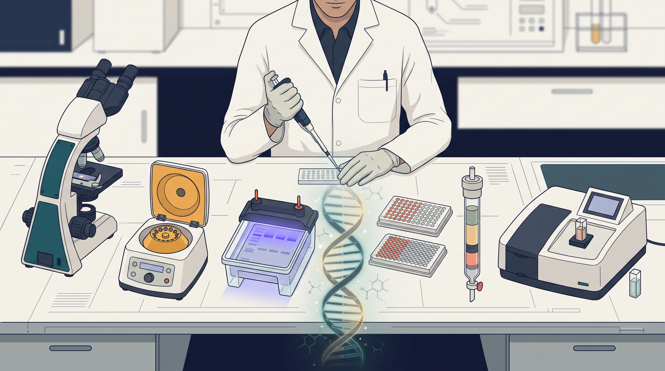
Fig. 12.0 – Tools of molecular biology.
Keep these five questions in mind as you read. Each one is answered somewhere in this chapter, and you will meet the answers exactly where the tools that provide them are explained.
12.1 Microscopy
Biological study begins with looking. The trouble is that almost everything a biologist wants to look at — a cell, a chromosome, a bacterium — is far too small for the unaided eye. Biological studies and explorations, therefore, cannot even be imagined without a microscope, because it lets us see something that lies completely beyond the reach of our eyes.
Microscopy today is no longer only about seeing a flat, enlarged picture. The technique has become so advanced that a researcher can not only view a highly magnified image of a very minute structure, but can also visualise the three-dimensional shape of that structure. Using powerful electron microscopic techniques, even the DNA molecule of bacteria and viruses has been visualised.
That last sentence is worth pausing on. A DNA molecule is roughly two nanometres wide. The fact that we can now form an image of it tells you how far the tool has travelled from the simple lens with which the story began.
Where the story begins
The use of the first microscope dates back to 1665, when the British physicist Robert Hooke designed a simple microscope using a combination of magnifying lenses (Fig. 12.1) and observed thin slices of cork. What he saw was a honeycomb-like arrangement of tiny empty boxes, and he coined the term ‘Cellulae’, or ‘cell’, for them.
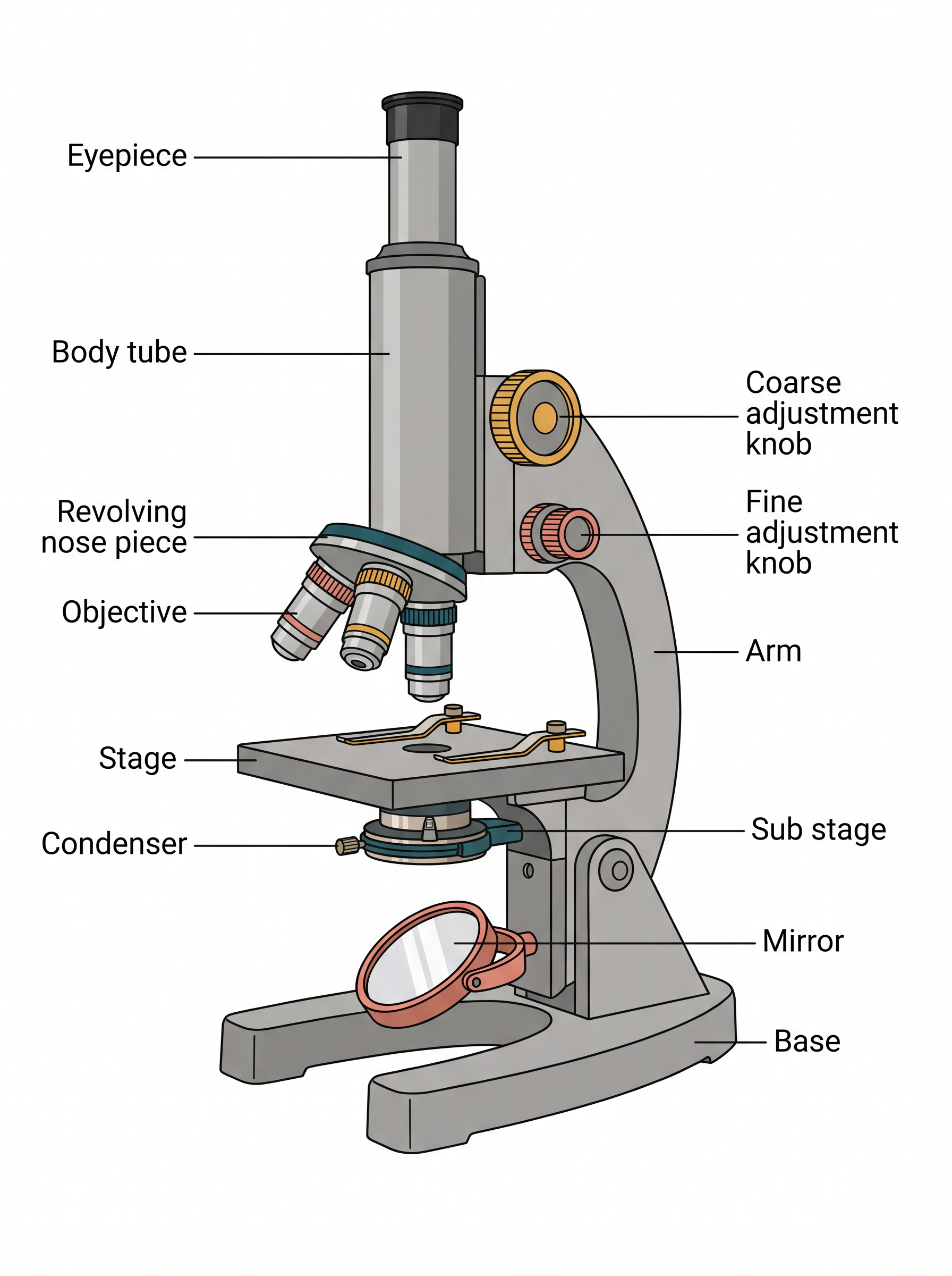
Fig. 12.1 – A compound microscope.
You are already aware that Matthias Jacob Schleiden and Theodor Schwann proposed the cell theory in 1838, on the basis of their observations of cells in plants and animals. Notice the order of events: the instrument came first, in 1665, and the great generalisation about all life being made of cells came almost two centuries later. The theory could not have been framed without the tool that made cells visible.
12.1.1 Magnification and Resolution
Let us now focus on the principle on which the technique of microscopy is based. Two optical properties are extremely important for an optical instrument like a microscope. One is the power to magnify, and the other is the ability to resolve. Students often treat these as the same thing, but they are quite different, and confusing them is a common source of error in examinations.
Magnification, or magnifying power, of a microscope is the ability by which the size of the retinal image can be increased. In simple terms, magnification is—
\[\text{Magnification} = \frac{\text{Size of retinal image with the help of microscope}}{\text{Size of the retinal image without using microscope}}\]
You may have studied in physics that the magnification (M) of a lens is measured by the following formula, in which \(f\) is the focal length of the lens and \(d\) is the distance of the object from the lens.
\[M = \frac{f}{f - d}\]
Here \(M\) is a pure number and has no unit, because it is a ratio of two lengths. Both \(f\) and \(d\) are lengths and are normally expressed in centimetres or millimetres. The formula tells us something useful: as the object is brought closer to the focal point, the denominator \((f - d)\) becomes smaller and the magnification rises sharply. This is exactly why the objective lens has to sit very close to the specimen.
Why a compound microscope has two lenses
Normally, the microscope used in the laboratory is a compound microscope, in which two sets of lenses are present. One is called the objective lens, which remains close to the object to be seen, and the other is the eyepiece, through which the observer looks.
It is needless to mention that the object, the objective lens, the eyepiece and the eye of the observer all have to lie along the same line, so that light can pass through the whole system and form the magnified image. If the alignment is disturbed, light simply does not reach the eye and the field goes dark.
In simple words, the magnification of a microscope is the product of the magnifying power of the objective lens and the magnifying power of the eyepiece (\(M_o \times M_e\)). This is why the two lenses are said to magnify in stages — the objective forms an enlarged image, and the eyepiece then enlarges that image again.
\[M = M_o \times M_e\]
Resolving power is the other important property of a microscope. It is the ability to form separate images of two objects situated very close to each other. It can be measured by the smallest distance between two points at which they are still seen as two points and not as one.
The smaller this distance, the better the resolving power. A microscope with poor resolving power will merge two neighbouring mitochondria into a single smudge, however large it makes them look.
12.1.2 Functioning of a light microscope
You have already studied the structure of a compound microscope in the previous class, but let us recapitulate it, because every later technique in this chapter is built on this basic arrangement.
As you can see in Fig. 12.1, a compound microscope consists of a base on which a stage is fitted, and the stage carries a central hole. Attached to the base is an arm, to which a body tube is fitted in such a way that it aligns with the hole of the stage. That alignment is not a detail of design — it is what allows light to travel straight from below the stage up into the eye.
At the lower end of the body tube, a nose piece is fitted, on which two to four objective lenses may be present. By rotating the nose piece, any one of the objective lenses can be brought directly above the hole in the stage, where the object to be seen has been placed on a glass slide. At the upper end of the body tube, an eyepiece is fitted, through which the observer views the specimen.
There are adjustment screws — coarse and fine — on the arm, which help in adjusting the distance of the objective lens from the object present on the stage. The coarse screw brings the specimen roughly into view; the fine screw makes the small final correction that sharpens the image. Recall from the magnification formula that image size depends on the object–lens distance, so these screws are doing real optical work, not merely moving parts about.
Below the stage there is a source of light, which may be a reflective mirror or a bulb. Its job is to illuminate the object and so make possible the formation of an image through the objective lens and the eyepiece (Fig. 12.2). In addition, a condenser is present between the light source and the stage, and it is important for focusing light onto the object. Without the condenser, the light spreads out and the specimen appears dim and low in contrast.
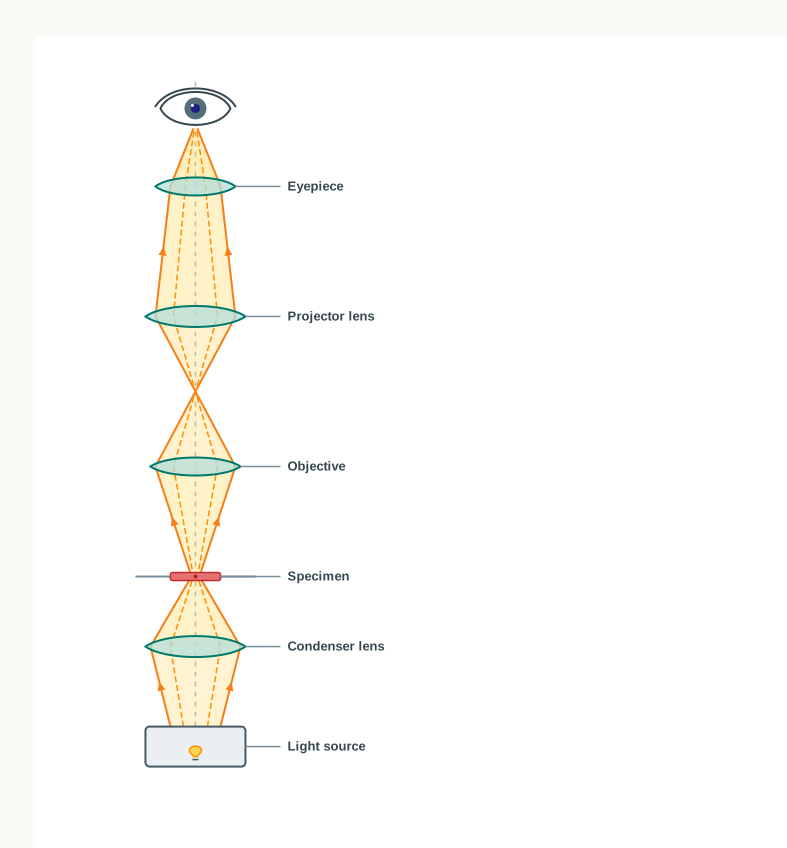
Fig. 12.2 – Pathway of light in a light microscope.
You might have observed that both objective lenses and eyepieces are available in different magnifying powers. In a student microscope, the eyepiece has a magnifying power of 10× or 15×, and the different objective lenses fitted on the nose piece are of 4×, 10×, 40/45× and 100×. Combining an eyepiece with different objectives therefore gives a range of total magnifications from the same instrument.
The technique of microscopy just discussed is also called bright field microscopy, because light is used to illuminate the object to be seen. The specimen appears as a dark shape against a bright background — hence the name.
This creates a practical problem. Most cells are nearly transparent, so different regions of the object look almost identical under plain light. Therefore, in order to distinguish different regions of the object, the specimen is stained with specific dyes or stains. Carmine, eosin, safranin, methylene blue, giemsa and a few others are commonly used stains for light microscopy.
12.1.3 Different forms of microscopy
Studying the minute details of the internal organisation of tissues and cells is so diverse a task that it cannot be achieved by light microscopy alone. Therefore, by making one or the other kind of manoeuvring — changing how the specimen is lit, what it is labelled with, or even what kind of radiation is used — quite diverse forms of microscopy have been developed. Each form solves a specific problem that ordinary bright field microscopy cannot solve.
Dark field microscopy
In one such manoeuvring, the light falling on the object from the central condenser is blocked by a disc, and the object is instead illuminated by an oblique light beam. This oblique beam is reflected off from the slide, and the image is illuminated against a dark background. Therefore, such a microscopy is known as Dark Field Microscopy.
The advantage is that only light scattered by the specimen itself reaches the eye, so even a faint, unstained structure stands out sharply. Mitochondria, nuclei, vacuoles and similar structures can be easily detected using this method.
Phase contrast microscopy
Similarly, in a different form called Phase Contrast Microscopy, the wave amplitude and phase of the light passing through the transparent object is changed. This change depends on the density of that part of the object or specimen.
Such a change is greater in the area where the density is comparatively high, and as a result of this, the varied contrast of different regions of the object can be seen. The instrument converts an invisible difference in density into a visible difference in brightness. This is especially helpful in the study of cell organelles and chromosomes, and it works on living, unstained cells — a real advantage, since staining usually kills the specimen.
Fluorescence microscopy
Staining of the object or specimen with some specific dye is routinely done, as you have seen. There are, however, some special types of dyes — for example acridine orange, bisbenzimide and merocyanine — which are also called fluorophores.
These dyes are capable of emitting light of longer wavelength after being illuminated, a property called fluorescence. As a result of this, the fluorophore-stained object looks more illuminated, and of a different colour depending on the dye used.
In fluorescence microscopy, the same principle is applied. The object to be seen is stained with a fluorophore in order to study a specific part of an organelle or molecule. After illuminating the object under the fluorescence microscope, the specifically stained region is easily seen or observed, glowing against a dark field while everything else stays dark.
This selectivity is the real power of the method: you see only what you have labelled. It is helpful in identifying bacteria or viruses to know the cause of an infection, and in immunodiagnosis. You will meet this same idea again later in the chapter, where fluorescent labels are used to mark a particular gene on a chromosome and to sort cells one by one.
Electron microscopy
Electron microscopy is a highly sophisticated technique in which the object to be studied is bombarded with an electron beam, which is approximately 1,00,000 times shorter in wavelength than visible light. This single fact is the whole reason for the technique’s existence: since resolution is limited by wavelength, using radiation of far shorter wavelength pushes the limit of resolution enormously downward.
The electron beam in an electron microscope magnifies the image with the help of electromagnetic lenses, rather than glass lenses. The entire passage of the electrons is in vacuum, because electrons would be scattered by air molecules and the image would be destroyed. The generated image is viewed on a fluorescent screen and not through an eyepiece, since the human eye cannot detect electrons directly.
Owing to the very much shorter wavelength of the electron, the image produced by an electron microscope is of very high resolution. Two types of electron microscopy are used: transmission electron microscopy and scanning electron microscopy.
In Transmission electron microscopy, an ultra-thin section of the object or specimen, coated with a heavy metal salt (of lead, tungsten, etc.), is placed in such a way that the electron beam passes through it to create the image. The heavy metal is needed because electrons pass too easily through light biological atoms; the metal scatters electrons and so creates contrast, and the section must be ultra-thin or no electrons would get through at all.
In the other technique of electron microscopy, the reflected electron beam from the gold- or platinum-coated surface of the object creates the image. In this technique, a highly magnified and resolved image of the object surface is generated, and therefore it is called Scanning electron microscopy.
Confocal microscopy
In the last few decades, yet another and more sophisticated microscopic imaging technique has been developed and used, called confocal microscopy. Confocal microscopy is useful in resolving detailed structures within fixed cells and tissues, and it gives sharp images of the objects.
The sharpness comes from the fact that light coming from outside the plane being examined is rejected, so the blur contributed by the layers above and below the focal plane is removed. To examine an object using confocal microscopy, it is first fluorescently labelled and then analysed under a confocal microscope in high resolution.
Choosing the right microscope
Board and competitive examinations rarely ask you to simply define these forms of microscopy. They far more often give you a purpose and ask which instrument you would choose — for instance, a resolved image of the surface of an object points to the scanning electron microscope, while internal ultrastructure points to the transmission electron microscope, and a living unstained cell points to phase contrast. Learning each technique together with the problem it was designed to solve is therefore far more useful than learning the names alone.
12.2 Centrifugation
You have studied about various biomolecules like proteins, nucleic acids and others that are present in the cells of all living organisms. To study any one of these biomolecules, you first have to get it out of the cell and away from everything else. That means you need to isolate it by using one or the other separation technique.
Centrifugation is one such technique. In it, particles or molecules are separated on the basis of their densities under the influence of gravitational force (g), by spinning them in a solution around an axis at high speed using centrifugal force.
Why spinning works
Left to itself in a test tube, a heavy particle will settle to the bottom under gravity alone — but for something as small as a mitochondrion or a protein, this may take days, and diffusion keeps stirring it back up. Spinning the tube rapidly around an axis creates a centrifugal force many times stronger than gravity, so the same settling happens within minutes instead of days. The technique does not change the physics of sedimentation; it simply speeds it up enormously.
The centrifuge
The equipment used is called a centrifuge (Fig. 12.3), and it is of different types depending on its use. It consists of a base, a rotating container (the spinning vessel or rotor) and a lid. The spinning vessel contains several centrifuge tubes.
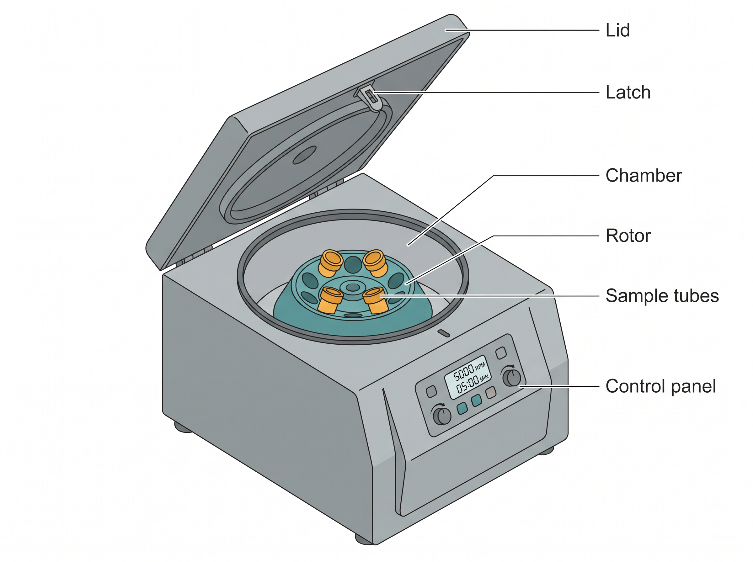
Fig. 12.3 – Basic structure of a centrifuge.
The cell extract or mixture is taken in the centrifuge tubes and allowed to spin at a desired speed — measured in revolutions per minute, or rpm — for a specific period of time. This leads to the settlement of the particulate material at the bottom of the centrifuge tubes. The settled material at the bottom is called the pellet, and the clear liquid left above it is the supernatant. Both are useful: sometimes the substance you want is in the pellet, and sometimes it is still in the supernatant.
Notice that two things must always be stated together for any centrifugation step — the speed and the time. Spinning too slowly, or for too short a time, leaves the wanted particle in the supernatant; spinning too fast, or for too long, drags unwanted material down along with it. A balanced load matters too, since an unevenly loaded rotor will vibrate violently at high speed.
12.2.1 Types of Centrifuge
Based on the principle and the application, the following types of centrifugations are performed—
Differential Centrifugation
Differential centrifugation is based upon the differences in the sedimentation rate (centrifugal force) of particles of different size and density. It is used to separate large cellular structures, the nuclear fraction, mitochondria, chloroplasts, or large proteins.
The working idea is straightforward. The extract is first spun at a low speed, which is just enough to bring down only the largest and heaviest structures. That pellet is kept aside, and the supernatant is spun again at a higher speed, bringing down the next-heaviest group. Repeating this in steps gives a series of fractions, each enriched in one kind of structure. This is why the method is called differential — the difference lies in the speed used at each step.
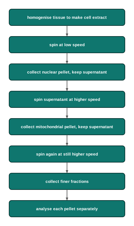
Fig. 12.4 – Differential centrifugation.
Density-gradient Centrifugation
In order to separate biological particles of similar size but differing in densities, one can use density gradient centrifugation. In this type of centrifugation, a density gradient is developed in the centrifuge tubes — that is, the liquid in the tube is arranged so that it becomes steadily denser from the top of the tube downwards.
Depending upon their densities, different molecules get sedimented at different levels within this gradient. The heavier molecules move outward and the lighter ones remain in the inner part of the centrifuge tubes. The greater the difference in density, the faster they move. Each species therefore stops where the surrounding liquid matches its own density, and forms a sharp band at that level rather than piling up at the bottom.
Ultracentrifugation
When centrifugation is carried out at very high speed, i.e., 100,000 x/g or more, to separate the molecules, it is called ultracentrifugation. At such enormous fields, even individual macromolecules such as proteins and nucleic acids — which stay suspended in an ordinary centrifuge — can be brought down and separated.
Commonly used centrifuges are:
- Table top/clinical centrifuge or microfuge
- High-speed centrifuge
- Ultracentrifuge
These three form a natural ladder of capability. The table top or clinical centrifuge, also called a microfuge, handles small tubes and modest speeds and is the everyday workhorse for spinning down cells or precipitates. The high-speed centrifuge reaches into the range needed for organelles. The ultracentrifuge, the most powerful and most expensive of the three, is reserved for macromolecules and for density-gradient work.
12.3 Electrophoresis
Electrophoresis is a method of separation on the basis of the charge to mass ratio of macromolecules under the influence of an electric field. Where centrifugation used density as its handle, electrophoresis uses electrical charge — and this gives it a completely different kind of resolving ability.
The name itself explains the method. Electrophoresis is a Greek word meaning ‘to bear electrons’. The prefix electro refers to electricity, which is required to migrate the molecules, and the suffix phoresis means ‘migration’ or ‘movement’.
Principle
Many important biological molecules, such as nucleotides, DNA, RNA, peptides and proteins, bear ionisable groups. Because of these groups, at any given pH they exist in solution as electrically charged species, either as cations or as anions.
Under the influence of an electric field, these particles will migrate either towards the cathode or towards the anode, depending on their net charge. A molecule carrying a net negative charge is pulled towards the positive electrode, and one carrying a net positive charge is pulled towards the negative electrode.
The mobility of a molecule is inversely proportional to its size and directly proportional to its charge, which is what allows different molecules to be separated from one another.
Read that relationship carefully, because both halves matter. A large charge pulls a molecule forward faster; a large size drags it back. Two molecules will separate only if they differ in at least one of these two properties. This single sentence explains everything that follows in this section — including why DNA behaves so conveniently and why proteins have to be specially treated first.
12.3.1 Agarose Gel Electrophoresis
In this type of electrophoresis, the gel is a matrix of agarose molecules that are held together by hydrogen bonds and form tiny pores. It is these pores that turn a simple electrical pull into a size-based separation, because a molecule must thread its way through them to move at all.
Gels for DNA separation are often made out of a polysaccharide called agarose, which comes as dry and powdered flakes. When the agarose is heated in a buffer and allowed to cool, it will form a solid and slightly squishy gel.
Setting up the gel
The gel is a slab of jelly-like material, placed in a gel box. One end of the box is connected to a positive electrode, and the other end to a negative electrode. The gel box is filled with a salt-containing buffer solution that can conduct current, so that the electric field is carried right through the gel and not merely across the empty box.
The end of the gel with the wells is positioned towards the negative electrode. The other end of the gel is positioned towards the positive electrode, to which the DNA fragments will migrate (Fig. 12.5).
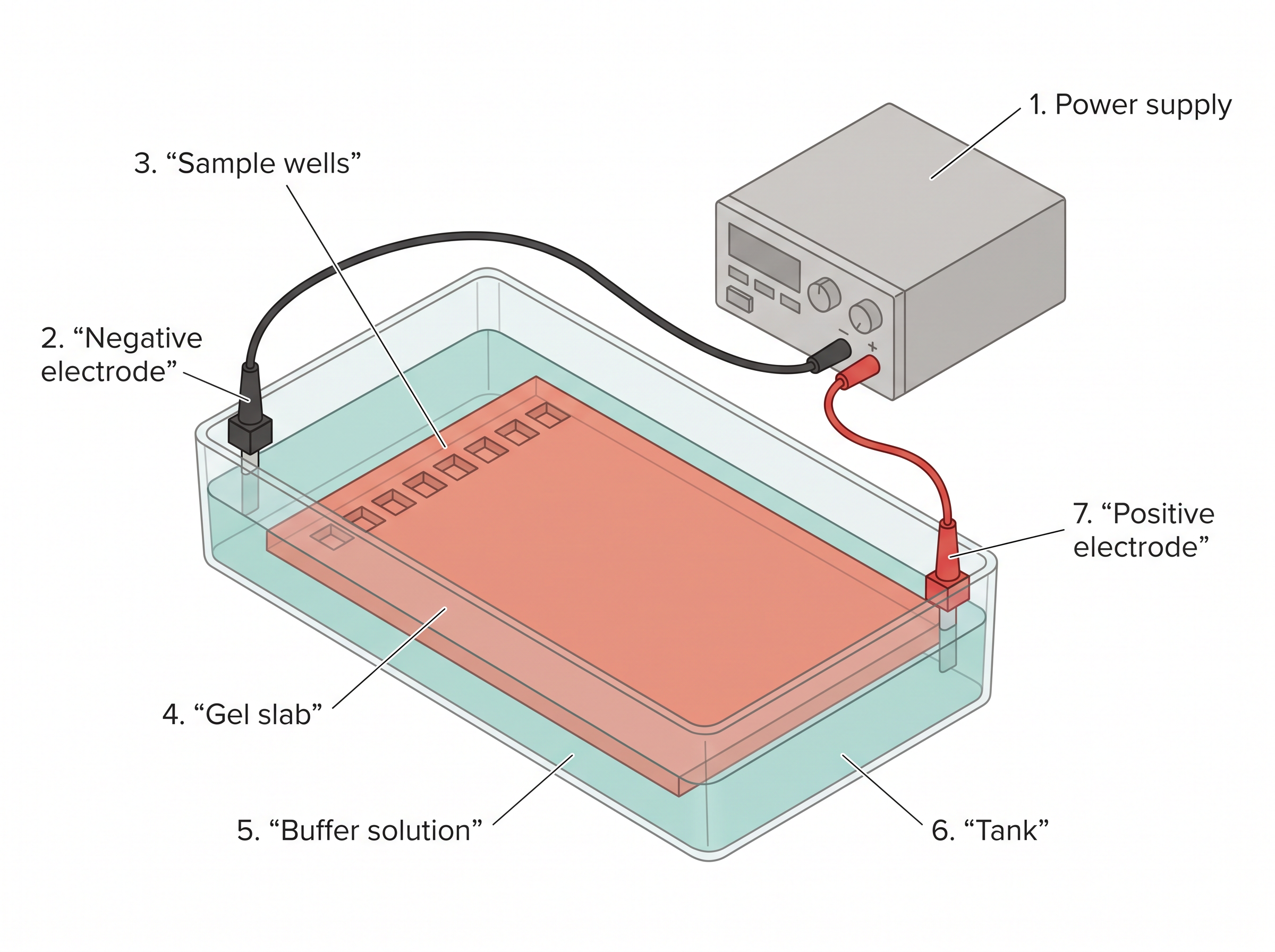
Fig. 12.5 – An agarose gel electrophoresis unit.
DNA molecules are negatively charged. Because of this, gel electrophoresis of DNA fragments separates them on the basis of size only. This is a fortunate simplification, and the reason is worth stating plainly: every DNA fragment, long or short, carries the same amount of negative charge per unit length, so charge and mass increase together and the charge to mass ratio stays practically constant. What is left to differ between fragments is only their length.
Using electrophoresis, we can check the different DNA fragments present in a sample and determine their absolute size with the help of a DNA ladder, which is made up of DNA fragments of known sizes. The ladder is run in a lane alongside the samples, and the unknown fragments are sized by comparing how far they have moved with the bands of the ladder.
Running the gel
When the power is turned on, the current begins to flow through the gel. DNA molecules have a negative charge due to the presence of phosphate groups in their sugar-phosphate backbone; therefore, they move through the matrix of the gel towards the positive electrode (anode).
The voltage for running an agarose DNA gel lies in the range of 80–120 V. As the electric current is applied, shorter pieces of DNA travel through the pores of the gel matrix faster than longer ones. Thus, the longest pieces of DNA remain near the wells, while the shortest pieces of DNA are close to the positive end of the gel.
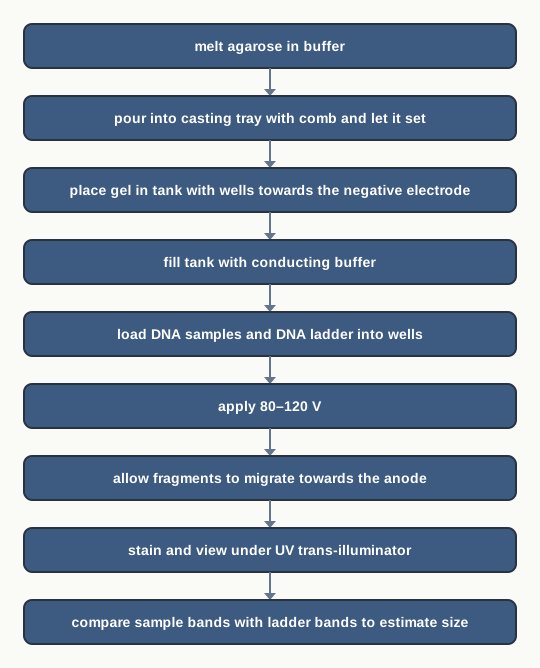
Fig. 12.6 – Agarose gel electrophoresis.
12.3.2 Visualising the DNA fragments
DNA is colourless, so at the end of a run there is nothing to see. The equipment used for the visualisation of target DNA is an ultra-violet (UV) trans-illuminator, which shines UV light up through the gel from below.
Ethidium bromide (EtBr) is most commonly used for staining DNA. This stain can be mixed into the gel mixture, or into the electrophoresis buffer, or the gel can be stained after it has been run — all three approaches are in use, and the choice is a matter of convenience.
Molecules of EtBr intercalate within the DNA bases — that is, they slide in between the stacked base pairs of the double helix — and fluoresce under UV light. Because the dye only fluoresces brightly when it is wedged into DNA, the bands glow while the rest of the gel stays dark (Fig. 12.7).
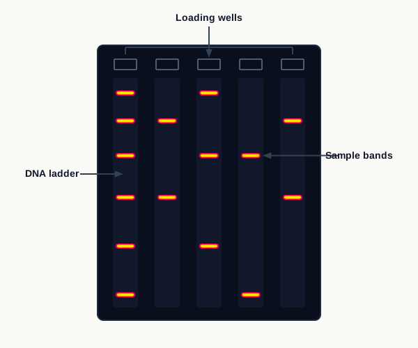
Fig. 12.7 – DNA bands on an agarose gel under UV light.
Despite its advantages, ethidium bromide is a potential carcinogen, so it must be handled with great care. The very property that makes it useful — its ability to slip between the base pairs of DNA — is also the reason it is hazardous, since it can insert itself into the DNA of the person handling it.
12.3.3 Polyacrylamide Gel Electrophoresis (PAGE)
PAGE is an analytical method used to separate the components of a protein mixture based on their size. Proteins present a difficulty that DNA does not, and the method is designed around it.
Different proteins carry different net charges at a given pH, and some are even positively charged. If they were simply run in an electric field, their migration would reflect a mixture of charge and size, and the result would be impossible to interpret in terms of size alone. To provide a uniform charge to the protein molecules, an anionic detergent called sodium dodecyl sulfate (SDS) is used to bind the proteins and give them a negative charge. Once every protein carries the same kind of charge in proportion to its length, the only remaining variable is size.
The proteins are then separated electrophoretically according to their size, using a gel matrix made of polyacrylamide in an electric field.
How the polyacrylamide matrix is made
Polyacrylamide is produced as a result of the polymerisation reaction between acrylamide and N,N’-methylene-bis-acrylamide (BIS), using a catalyst. BIS is the cross-linker: it ties neighbouring acrylamide chains to one another and so turns a set of long chains into a three-dimensional mesh.
The degree of polymerisation, or cross-linking, can be controlled by adjusting the concentration of acrylamide and BIS. The more the cross-linking, the harder the gel. This gives the experimenter direct control over pore size, which is the key advantage of polyacrylamide over agarose for protein work.
Hardness of the gel, in turn, modulates the friction experienced by macromolecules when they travel through the gel during PAGE, thus affecting the resolution of separation. Loose gels (4–8% acrylamide) allow higher molecular weight molecules to migrate faster through the gel, while hard gels (12–20% acrylamide) restrict the migration of large molecules and selectively allow small ones to move through the gel.
The practical rule that follows is one that examination questions return to repeatedly: choose a loose, low-percentage gel when you need to resolve large proteins, and a hard, high-percentage gel when the proteins of interest are small. A mixture spanning both extremes is poorly served by either single choice.
12.3.4 Tracking dye
As DNA, RNA and proteins are mostly colourless, their progress through the gel during electrophoresis cannot be easily followed. There is no way of telling by eye how far the run has gone — and if the run is continued too long, the samples travel off the end of the gel and are lost.
Anionic dyes of a known electrophoretic mobility are usually included in the sample buffer. Because their mobility is known, their visible position acts as a marker for the invisible position of the samples.
A very common tracking dye is bromophenol blue. This dye is coloured at alkali and neutral pH, and is a small negatively charged molecule that moves towards the anode. Being a highly mobile molecule, it moves ahead of most proteins and nucleic acids. As it reaches the anodic end of the electrophoresis medium, electrophoresis is stopped — the dye front is the signal that the run is complete.
Other common tracking dyes are xylene cyanol, which has lower mobility, and Orange G, which has a higher mobility. Since the three dyes travel at different speeds, using more than one of them together gives several reference points down the gel instead of just one.
Visualisation of protein on gel
Coomassie Brilliant Blue R-250 is the most popular protein stain. It is an anionic dye, which binds non-specificially to proteins — that is, it binds to proteins in general rather than to any particular one, which is exactly what is wanted when every band on the gel needs to be seen.
Proteins in the gel are fixed by methanol and acetic acid and are simultaneously stained. Fixing is important because it precipitates the proteins in place within the gel; without it, they would slowly diffuse out and the bands would blur.
The excess dye incorporated into the gel can be removed by destaining with the same solution without the dye. The proteins are detected as blue bands on a clear background.
After the visualisation by a staining (protein-specific) technique, the size of a protein can be calculated by comparing its migration distance with that of a known molecular weight ladder — exactly the same logic used for sizing DNA fragments against a DNA ladder.
12.4 Enzyme-linked Immunosorbent Assay (ELISA)
Enzyme-linked immunosorbent assay (ELISA) was invented by two Swedish scientists, Eva Engvall and Peter Perlman, in 1971. ELISA is a quantitative method used for the measurement of antigen and antibody concentration in a given sample.
Before going further, it is worth fixing two terms. An antigen is any molecule that the immune system recognises as foreign — a protein on the surface of a virus, for example. An antibody is a protein made by the immune system that binds to one particular antigen and to almost nothing else. That exquisite specificity is the whole foundation of this technique: an antibody will pick out its own antigen even from a complicated mixture such as blood serum.
Turning a binding event into a colour
The difficulty is that when an antibody binds its antigen, nothing visible happens. ELISA solves this by attaching a reporter to the binding event.
The measurement is done by monitoring the antigen–antibody interaction with the help of an enzyme catalysed reaction. This detection system — an enzyme-conjugate — is covalently linked to a specific antibody that recognises a target antigen. Wherever that antibody binds, the enzyme is carried along with it and stays behind; wherever it does not bind, the enzyme is washed away.
A colourless substrate is then added. The enzyme converts it into a coloured product, so a binding event that was invisible becomes a colour that can be seen and, more importantly, measured. The intensity of the colour produced is detected by an ELISA reader or a spectrophotometer.
Because the enzyme keeps turning over substrate molecules for as long as it is left to act, one bound antibody can generate a very large number of coloured product molecules. This built-in amplification is why ELISA can detect quantities far too small to be seen by any direct method. ELISA is also a safer and less costly assay as compared to many other immunological assays, since it needs no radioactive label.
The assay is carried out in a microtiter plate — a small plastic tray carrying dozens of tiny wells, so that many samples, along with the controls, can be run side by side under identical conditions.
Reading the result quantitatively
A number of modifications of ELISA have been developed, allowing qualitative detection or quantitative measurement of either antigen or antibody. These different types of ELISA can be employed qualitatively to detect the presence of an antibody or antigen — that is, simply to answer “is it there or not”.
To go further and answer “how much is there”, known concentrations of antibody or antigen are run in some of the wells, and a standard curve is prepared from the colour intensities they give. The unknown sample’s colour intensity is then read against this curve to determine its concentration.
Direct ELISA
In direct ELISA, the antigen or sample is coated on the microtiter plate wells, and the enzyme-conjugated antibody ‘directly’ binds to the antigen. The enzyme linked to the antibody reacts with its substrate to produce a colourful product that can be measured using a spectrophotometer or ELISA reader.
The direct ELISA is faster and less error prone, and it does not require a secondary antibody. With only one antibody step, there are fewer incubations and fewer washes, and fewer opportunities for something to go wrong.
The disadvantage of direct ELISA is non-specific binding of the antibody due to cross-reactivity — the labelled antibody may attach weakly to molecules other than its intended target, producing colour that does not represent the antigen being measured.
Indirect ELISA
The indirect ELISA detects the presence of an antibody in a sample, and it does so in two stages (Fig. 12.8).
Firstly, an unlabelled primary antibody (Ab1) is applied to antigen-coated microtiter wells. If the sample contains antibodies against that antigen, they bind; the unbound extra primary antibody (Ab1) is then washed off. The washing step is not a formality — without it, unbound antibody would remain in the well and generate colour that has nothing to do with genuine binding.
Next, an enzyme-conjugated secondary antibody (Ab2), specific for the primary antibody (Ab1), is added. Any unbound secondary antibody (Ab2) is washed off, and the substrate is added. The amount of coloured product formed can be measured using a spectrophotometer or ELISA reader.
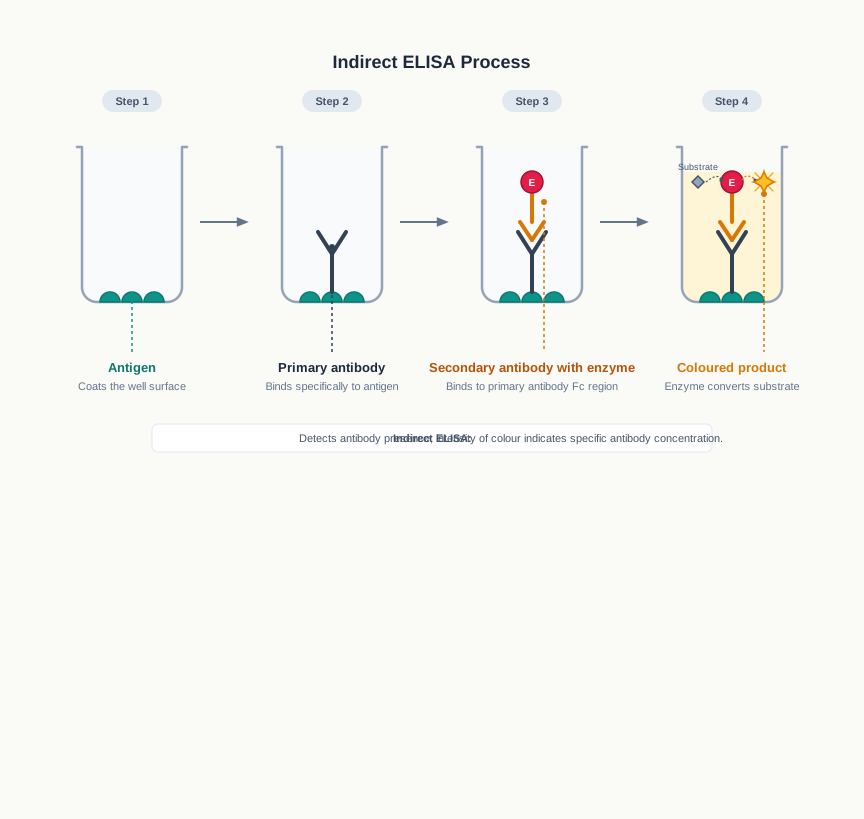
Fig. 12.8 – Indirect ELISA.
Indirect ELISA has increased sensitivity, since more than one labelled antibody is bound per primary antibody. Each primary antibody offers several sites for secondary antibodies to attach, so several enzyme molecules are recruited for every single antigen–antibody binding event, and the signal is multiplied.
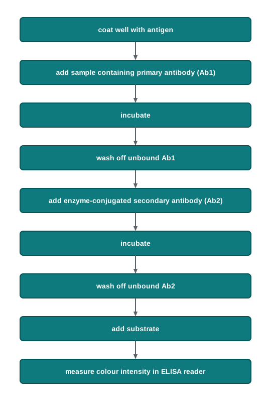
Fig. 12.9 – Steps in indirect ELISA.
Sandwich ELISA
In sandwich ELISA, the antibody is coated on the microtiter plate, and this coated antibody is referred to as the captured antibody. Using the sandwich ELISA technique, the antigen can be detected or measured (Fig. 12.10).
After the captured antibody is coated on the plate, the antigen is added and allowed to react with the captured antibody. Excess antigen is washed off, and then a second enzyme-conjugated antibody, specific for a different epitope on the antigen, is loaded. An epitope is the part of an antigen molecule to which an antibody attaches.
The reason the second antibody must recognise a different epitope is straightforward: the first epitope is already occupied by the captured antibody. If both antibodies competed for the same site, the second one could never bind, and no colour would ever develop. The antigen ends up held between two antibodies — which is exactly why the method is called a sandwich.
The excess unbound enzyme-conjugated antibody is washed off, substrate is added, and the coloured product produced is then measured using a spectrophotometer or ELISA reader.
High specificity, and no requirement of antigen purification or limiting antigen, are the main advantages of sandwich ELISA. Because the antigen has to be recognised by two different antibodies before any colour appears, a molecule that resembles the target only slightly will fail at one step or the other. This also means the sample can be applied as it is, without first being purified.
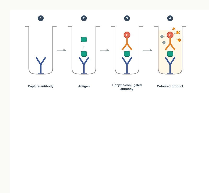
Fig. 12.10 – Sandwich ELISA.
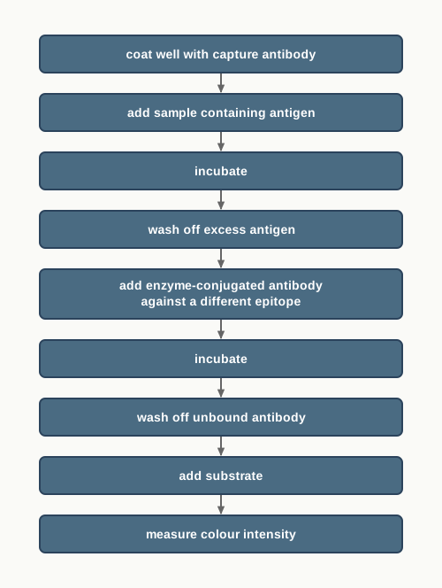
Fig. 12.11 – Steps in sandwich ELISA.
Competitive ELISA
The competitive ELISA helps in measuring amounts of antigen (Fig. 12.12). Its logic runs in the opposite direction to the other formats, and this reversal is what students most often get wrong.
In this method, the antibody and antigen are first incubated in solution. In this step the antibody is present in excess to the antigen; the antigen will bind to its antibody in a concentration dependent manner, leaving unbound antibody accordingly. In other words, the more antigen the sample contained, the less free antibody is left over at the end of this incubation.
This antigen–antibody complex is then added to an antigen-coated microtiter well. Only the antibody that is still free can attach to the antigen already fixed on the well surface; antibody that is already occupied cannot. Thus, if more antigens are present in the sample, less free antibody will be available to bind to the antigen-coated well, and vice versa.
Finally, the enzyme-conjugated secondary antibody (Ab2), specific for the primary antibody, is added to the plate, and these bind to the primary antibody bound to the antigen on the plate. As in the case of indirect ELISA, the addition of an enzyme-conjugated secondary antibody (Ab2) specific for the primary antibody helps in determining the amount of primary antibody bound to the well.
Thus, in the competitive ELISA, the higher the concentration of antigen in the sample, the lower will be the free antibody, and accordingly the intensity of the developed colour will be less. The relationship between antigen concentration and colour is therefore inverse — a pale well means a great deal of antigen, and a deeply coloured well means very little.
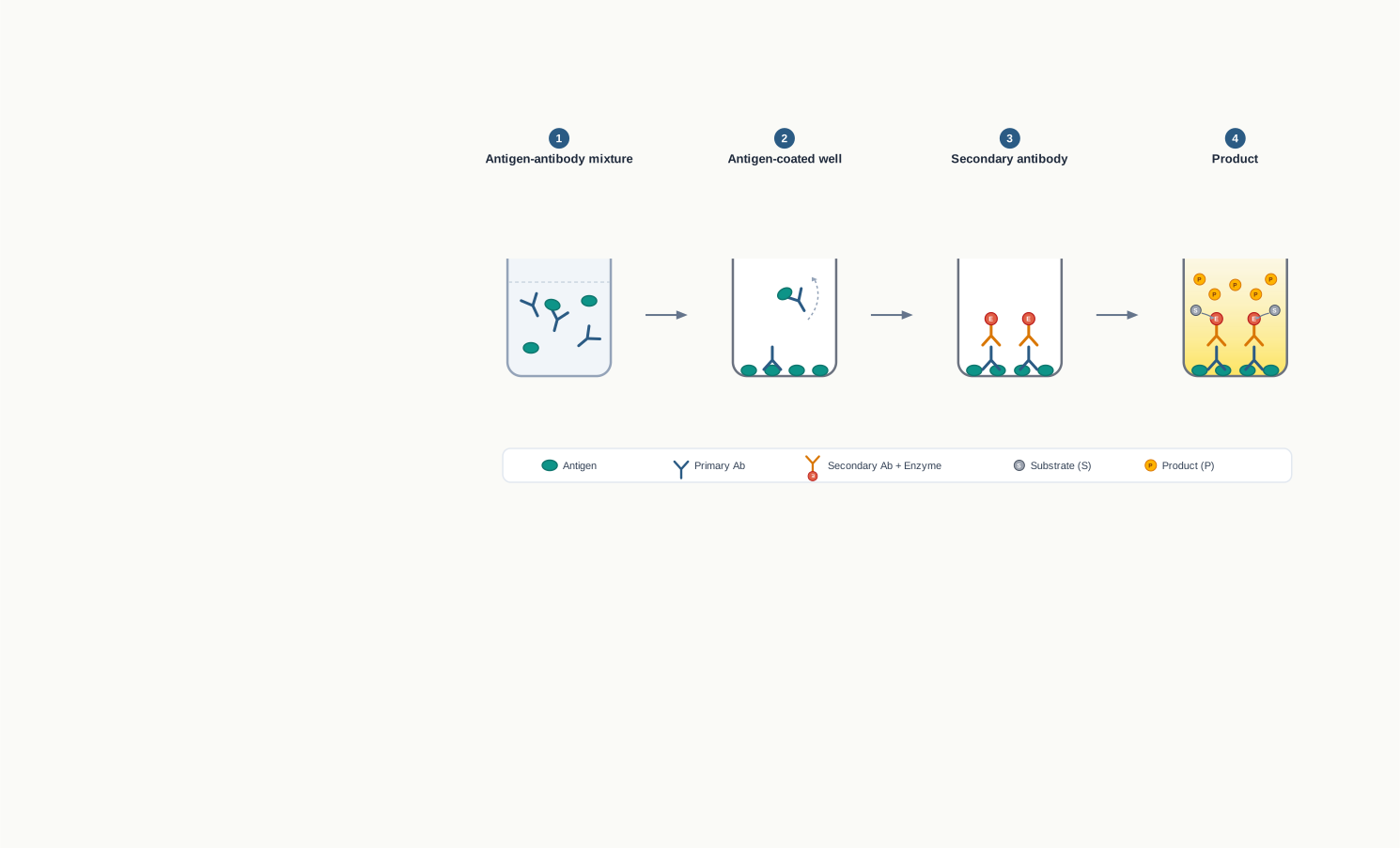
Fig. 12.12 – Competitive ELISA.
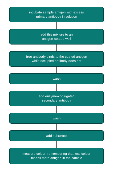
Fig. 12.13 – Steps in competitive ELISA.
Application of ELISA
- The presence of an antigen or antibody in a sample can be estimated.
- Concentration determination of serum antibody in a virus test can be carried out.
- Detection of potential food allergens in the food industry.
- Disease outbreaks can be tracked down, e.g., HIV, bird flu, cholera, etc.
Each of these applications rests on the same two properties. The specificity of the antibody decides what is detected, and the amplifying action of the enzyme decides how little of it can be detected. In food testing, for instance, an allergen such as peanut protein must be picked out from a complex processed food at trace levels — a task no ordinary chemical test could manage.
### 12.9.1 DNA sequencing methods


Historically there are two main methods of DNA sequencing, namely, (1) the Enzymatic method (Sanger's method, dideoxynucleotides chain termination method) and (2) the Chemical degradation method (Maxam and Gilbert method).

The names capture the essential contrast between them. The enzymatic method *builds* new DNA strands and stops them at known points; the chemical method *breaks* an existing strand at known points. Both end up with a collection of fragments of different lengths, and in both cases the sequence is deduced from the sizes of those fragments.

The two methods are described in detail in the following sections:

###### (a) Sanger's method {.unnumbered .unlisted}


Sanger's method works on the principle that dideoxynucleotides — dideoxyadenine, dideoxyguanine and so on, which resemble normal nucleotides but lack the normal –OH group at the 3' position — get incorporated, instead of the normal deoxynucleotide, into the newly synthesised chain (the daughter chain). This leads to termination of the synthesis of the new strand at that point, and hence it is called the chain termination method (Fig. 12.14).

<img src="images/fig12.14.svg" onerror="this.onerror=null; this.src='images/fig12.14.png';" alt="Fig. 12.14">

::: {.figure-caption}
Fig. 12.14 – Structure of a deoxynucleotide and a dideoxynucleotide.
:::


The chemistry behind the termination is worth being clear about, because it is the single idea on which the whole method rests. A growing DNA chain is extended by forming a bond between the 3'–OH group of the last nucleotide and the incoming nucleotide. A dideoxynucleotide has no –OH at its 3' position, so once it has been added there is simply nothing for the next nucleotide to attach to, and that strand can grow no further.

::: {.callout-note .box-definition icon=false title="Definition"}

*A dideoxynucleotide is a nucleotide that lacks the –OH group at the 3' position of its sugar, so that once it is incorporated into a growing DNA chain, no further nucleotide can be added and synthesis stops at that point.*

:::


Sanger's method is considered as a gold standard for DNA sequencing. It is used even today for routine sequencing applications, and also for the validation of Next Generation Sequencing data, which you will read about at the end of this section.

###### Setting up the reaction {.unnumbered .unlisted}


In Sanger's method of DNA sequencing, the template DNA — the DNA whose sequence has to be determined — is mixed with a primer complementary to the template DNA, and with the four normal dNTPs, one of which is labelled radioactively or fluorescently.

A **primer** is a small piece of chemically synthesised DNA of defined sequence that can pair with the template DNA to act as a starting point for DNA synthesis. It is needed because DNA polymerase cannot begin a chain from nothing; it can only *extend* an existing chain. The primer also fixes where the reading begins, so that every new strand starts from the same point and the fragment lengths can be meaningfully compared.

This mixture is then split into four different tubes that are labelled A, C, G and T. Each tube is then 'spiked' with a different ddNTP — ddATP for tube A, ddCTP for tube C, ddGTP for tube G, or ddTTP for tube T.

Following this, DNA polymerase is added, and using the DNA template and its complementary primer, the synthesis of new strands of DNA complementary to the template begins.

Occasionally, a dideoxynucleotide is added instead of the normal deoxynucleotide, and synthesis of that strand is terminated at that point. The word "occasionally" is doing important work here. Because each tube contains far more of the normal nucleotide than of the dideoxynucleotide, termination happens only now and then, and at a different position in each individual molecule. Across the millions of molecules in the tube, every possible stopping position is represented — which is exactly what is needed.

Thus, all fragments in lane A will end in an A, fragments in lane C will all end in a C, fragments in lane G will all end in a G, and fragments in lane T will all end in a T.

::: {.callout-note .box-sidebar icon=false title="Exam Corner" collapse="true"}

**Q. What would happen if a tube were spiked with dideoxynucleotide only, and no normal nucleotide of that base at all?**

A. Every single strand would terminate at the very first position where that base was required, so the tube would contain fragments of only one length. All the information about the further positions of that base would be lost. The whole method depends on the *ratio* of normal to dideoxynucleotide being such that termination is occasional rather than certain.

:::


###### Reading the result {.unnumbered .unlisted}


After carrying out the reaction for a fixed time, the newly synthesised DNA strands (fragments) are separated through high resolution polyacrylamide gel electrophoresis (PAGE), and the DNA fragments are visualised by exposing the gel to X-ray film for nucleotides labelled radioactively.

PAGE is used here rather than an agarose gel for a demanding reason: the fragments to be told apart differ in length by a single nucleotide, and only a high-resolution polyacrylamide gel can resolve such a difference.

Finally, the sequence of the DNA is read from the gel by starting from the bottom and reading upward on the X-ray film (Fig. 12.15). Reading upward gives the sequence in the 5'→3' direction of the newly made strand, because the shortest fragment — the one that has travelled farthest down the gel — represents the base nearest the primer, and each band above it adds one more base.

<img src="images/fig12.15.svg" onerror="this.onerror=null; this.src='images/fig12.15.png';" alt="Fig. 12.15">

::: {.figure-caption}
Fig. 12.15 – Sanger's method of DNA sequencing.
:::


Study the gel in Fig. 12.15 the way an examiner will expect you to. Find the lowest band anywhere across the four lanes, and note which lane it lies in — that lane's letter is the first base. Move up to the next-lowest band in any lane and read off its letter, and continue upwards. Two bands at the same height in different lanes would mean the run has failed, since a fragment of a given length can end in only one base.

<img src="images/fig12.16.svg" onerror="this.onerror=null; this.src='images/fig12.16.png';" alt="Fig. 12.16">

::: {.figure-caption}
Fig. 12.16 – Sanger's chain termination sequencing.
:::


::: {.callout-note .box-technique icon=false title="Technique" collapse="true"}

Sanger's method (dideoxy chain termination sequencing)
Principle: A dideoxynucleotide lacks the 3'–OH group needed to extend a DNA chain, so wherever one is incorporated, synthesis stops; running four such reactions, each stopped by a different base, produces sets of fragments whose lengths reveal the position of every base.
Steps: Mix template, primer, DNA polymerase and labelled dNTPs → divide into four tubes → add a different ddNTP to each → carry out synthesis for a fixed time → separate the fragments by high resolution PAGE in four lanes → visualise by autoradiography → read the sequence from the bottom of the gel upwards.
Used for: Determining the base sequence of a DNA fragment; it remains the gold standard, and is used today both for routine sequencing and to validate data from newer methods.

:::


::: {.callout-note .box-compare icon=false title="Compare Table" collapse="true"}

Deoxynucleotide (dNTP) vs Dideoxynucleotide (ddNTP)
| Feature | dNTP | ddNTP |
|---|---|---|
| Group at the 3' position of the sugar | –OH | –H; the –OH is missing |
| Can the next nucleotide be added after it? | Yes | No |
| Effect on the growing chain | Chain continues to elongate | Chain synthesis is terminated at that point |
| Relative amount used in a Sanger reaction | Present in large excess | Present in small amount, so that termination is occasional |

:::


###### (b) Chemical Degradation Method (Maxam and Gilbert Method) {.unnumbered .unlisted}


In the chemical degradation method of DNA sequencing, the DNA fragment whose sequence is to be determined is cleaved in a base specific manner using chemicals, as shown in Fig. 12.17.

Before the chemical mediated degradation of the DNA, the DNA is labelled at the 5' end using the enzyme polynucleotidyl kinase and a gamma-³²P labelled nucleotide. Labelling one end only is essential: it means that on the film, only those fragments that include the labelled end will appear, so every visible band can be measured from the same fixed starting point.

The chemicals are chosen so that each attacks one base, or one pair of bases, and not the others:

<img src="images/fig12.17.svg" onerror="this.onerror=null; this.src='images/fig12.17.png';" alt="Fig. 12.17">

::: {.figure-caption}
Fig. 12.17 – Cleavage reactions in the Maxam and Gilbert method.
:::


The fragments generated are subsequently separated using high resolution PAGE to resolve the sequence order. These gels are placed under X-ray film, which then yields a series of dark bands that show the location of the radiolabeled DNA fragments. The fragments are ordered by size, and therefore we can deduce the sequence of the DNA molecule.

The logic of reading is the mirror image of the Sanger gel. There, a band in lane A meant a strand that had been *stopped* at an A; here, a band in the G lane means a strand that has been *cut* at a G. In both cases the length of the fragment locates that base along the molecule.

::: {.callout-note .box-technique icon=false title="Technique" collapse="true"}

Maxam and Gilbert method (chemical degradation sequencing)
Principle: Specific chemicals cleave DNA at specific bases; if the DNA is first labelled at one end, the sizes of the resulting labelled fragments reveal the positions of those bases along the molecule.
Steps: Label the DNA at the 5' end using polynucleotidyl kinase and a gamma-³²P labelled nucleotide → divide the sample and treat each portion with a base-specific chemical (DMS with heat for G, DMS with acid for A, hydrazine with high NaCl for C, hydrazine for C+T) → separate the fragments by high resolution PAGE → expose the gel to X-ray film → order the bands by size and deduce the sequence.
Used for: Determining DNA sequence by chemical cleavage; historically important, and useful where the DNA cannot conveniently be copied by a polymerase.

:::


::: {.callout-note .box-compare icon=false title="Compare Table" collapse="true"}

Sanger's method vs Maxam and Gilbert method
| Feature | Sanger's method | Maxam and Gilbert method |
|---|---|---|
| Type of method | Enzymatic; also called the dideoxynucleotide chain termination method | Chemical degradation method |
| Basic action on DNA | New strands are synthesised and terminated at specific bases | The existing strand is cleaved at specific bases |
| Key reagents | Primer, DNA polymerase, dNTPs and ddNTPs | Dimethylsulphate and hydrazine, used under different conditions |
| Requirement of a primer and polymerase | Both required | Neither required |
| Labelling | One of the dNTPs is labelled radioactively or fluorescently | The DNA is labelled at the 5' end with gamma-³²P |
| Separation and reading | High resolution PAGE, read from the bottom of the gel upwards | High resolution PAGE, fragments ordered by size |
| Present status | Gold standard; still in routine use and used to validate newer data | Largely historical; uses hazardous chemicals |

:::


### 12.9.2 Automated DNA sequencing


The majority of DNA sequencing is now done through the automated method. These automated sequencers primarily work on the Sanger method of DNA sequencing — the principle has not changed, only the way it is carried out and read.

In automated sequencing, fluorescent labelled dideoxynucleotides are used, which has eliminated the need for radioactive isotopes. This removes both the safety hazard of handling radioactivity and the long wait for an X-ray film to be exposed and developed.

The slab gel has been replaced by polymer-filled capillary tubes in automated equipment. A narrow capillary dissipates heat far better than a thick slab, so higher voltages can be used and the run is completed much faster.

Automation of DNA sequencing has made the method much quicker and more reliable. For example, in one year, by using manual sequencing, on an average, a person can sequence 20,000 to 50,000 bases, while an automated sequencer can sequence that long in just a few hours. Furthermore, the total cost of material for one gel using the automated method is approximately half, compared to that of the manual method.

###### One tube instead of four {.unnumbered .unlisted}


In automated DNA sequencing, all four dideoxy reactions are carried out in a single tube. This is possible because each dideoxynucleotide is labelled with a different fluorescent dye, such as Rhodamine 110 (RHO)-A, which gives green fluorescence; Rhodamine 6G (REG)-C, which gives blue fluorescence; Tetramethyl Rhodamine (TAMRA)-G, which gives black fluorescence; and X-Rhodamine (ROX)-T, which gives red fluorescence.

This is the essential change. In the manual method, the identity of a base was given by *which lane* the band appeared in, and four lanes were therefore needed. In the automated method, the identity is given by the *colour* of the label, so the four sets of fragments can be mixed together without any loss of information.

The contents of the single tube reaction are loaded onto a single lane of a gel and electrophoresis is done. The sequence is determined by the order of the dyes coming off the gel.

A fluorimeter and a computer are hooked up to the gel, and they detect and record the fluorescent dye attached to the fragments as they come off the gel. All the DNA fragments labelled with a fluorescent dideoxynucleotide are 'read' by a laser, and the fluorescence intensity is translated into a data 'peak' (Fig. 12.18).

<img src="images/fig12.18.svg" onerror="this.onerror=null; this.src='images/fig12.18.png';" alt="Fig. 12.18">

::: {.figure-caption}
Fig. 12.18 – Chromatogram of automated sequencing.
:::


Notice that the output is no longer a picture of a gel to be read by eye, but a chromatogram of peaks — one peak per base, each in the colour of the dye that terminated that fragment. A clean, evenly spaced series of single-coloured peaks indicates a reliable read; broad, overlapping or double peaks indicate that the read at that position cannot be trusted.

::: {.callout-note .box-numerical icon=false title="Numerical 12.8" collapse="true"}

**A laboratory needs to sequence a bacterial genome of 4.6 × 10⁶ bases. (a) Taking the upper figure quoted above, that a person sequencing manually can complete 50,000 bases in one year, how many years of manual work would this genome require? (b) An automated sequencer completes 50,000 bases in 5 hours. How many days of continuous running would the same genome need? (c) Comment on what this comparison implies for the feasibility of whole-genome projects before automation.**

:::


::: {.callout-note .box-scenario icon=false title="Scenario" collapse="true"}

A student is shown two sequencing outputs from the same DNA sample — one an X-ray film with four lanes of dark bands, and the other a printed chromatogram of coloured peaks. Asked which method produced each, and why the second needs only one lane, the answer lies entirely in how the base is identified: by position in the manual method, by colour in the automated one. Questions of this pattern, giving an output and asking you to infer the method, are common in application-based papers.

:::


::: {.callout-note .box-sidenote icon=false title="Side Note" collapse="true"}

**Next-generation Sequencing (NGS).** NGS methods have facilitated the sequencing of very large DNA, such as a whole genome, because the methods described above work optimally for short sequence analysis up to a few Kb size DNA, and it is difficult to analyse a whole genome by them as it will take too much time and cost. The evolution of DNA sequencing from the historical methods of Sanger (Sanger sequencing) and Maxam & Gilbert (Maxam-Gilbert sequencing) to today's high-throughput technologies has occurred at a breathtaking speed. In the past 30 years or so, these high-throughput technologies have given rise to super-exponential growth in sequence data generation, and the resultant data have led to transformative applications ranging from basic biology to criminal investigation and prenatal diagnostics. NGS allows massively parallel sequencing reactions, and therefore these platforms are capable of analysing millions or even billions of sequencing reactions at the same time. The widely used NGS platforms are Roche/454 sequencing, Solexa/Illumina and SOLiD platforms.

:::


::: {.callout-note .box-bioethics icon=false title="Bioethics" collapse="true"}

Who should have access to a person's genome sequence?
Sequencing has become fast and cheap enough that an individual's whole genome can be read for diagnosis, for research, or out of simple curiosity. The benefits are real: an inherited disease risk can be identified long before symptoms appear, and drug choices can be matched to a person's own genetic makeup. But a genome sequence is unusually revealing. It discloses risks the person may not have wished to know, it discloses information about relatives who consented to nothing, and once it has leaked it cannot be recalled or altered. Concerns have been raised about insurers or employers gaining access to such data, and about the long-term storage of samples and sequences in biobanks. The safeguards usually proposed are informed consent that states clearly what will be looked for and what will be reported back, a recognised right not to be told incidental findings, strict de-identification of stored data, and legal limits on the use of genetic information in insurance and employment. Different countries have struck this balance differently, and the debate is far from settled.

:::
This chapter was long enough to split to ensure nothing is cut off. This is Part A, ending just before the DNA Microarray section. Reply to continue, and I will process Part B, merge them automatically, and run the final unbroken sequence renumbering.