Chapter 10: Protein Informatics and Cheminformatics

In the early 1960s, the biochemist Christian Anfinsen did something to an enzyme that looked almost like destruction. He took ribonuclease, a small protein with a precise three-dimensional shape, and treated it with chemicals that broke the bonds holding that shape together. The enzyme unfolded into a limp chain and stopped working. Then he removed those chemicals — and the chain folded itself back into exactly the same shape and started working again. Nobody had guided it. The conclusion was remarkable: every instruction needed to build the final 3D structure was already written into the order of amino acids in the chain. Anfinsen received a Nobel Prize for this work in 1972.

That raised an obvious question. If the instructions are in the sequence, can a computer read the sequence and tell us the shape — without a laboratory at all? For nearly fifty years the answer was “not reliably”. Then, in 2020, a computer program called AlphaFold predicted protein structures with an accuracy close to laboratory methods, and in 2024 that line of work was recognised with a Nobel Prize in Chemistry.

Today the same computational thinking is used on medicines: a computer can sift through billions of chemical structures and shortlist the few worth making in a laboratory.

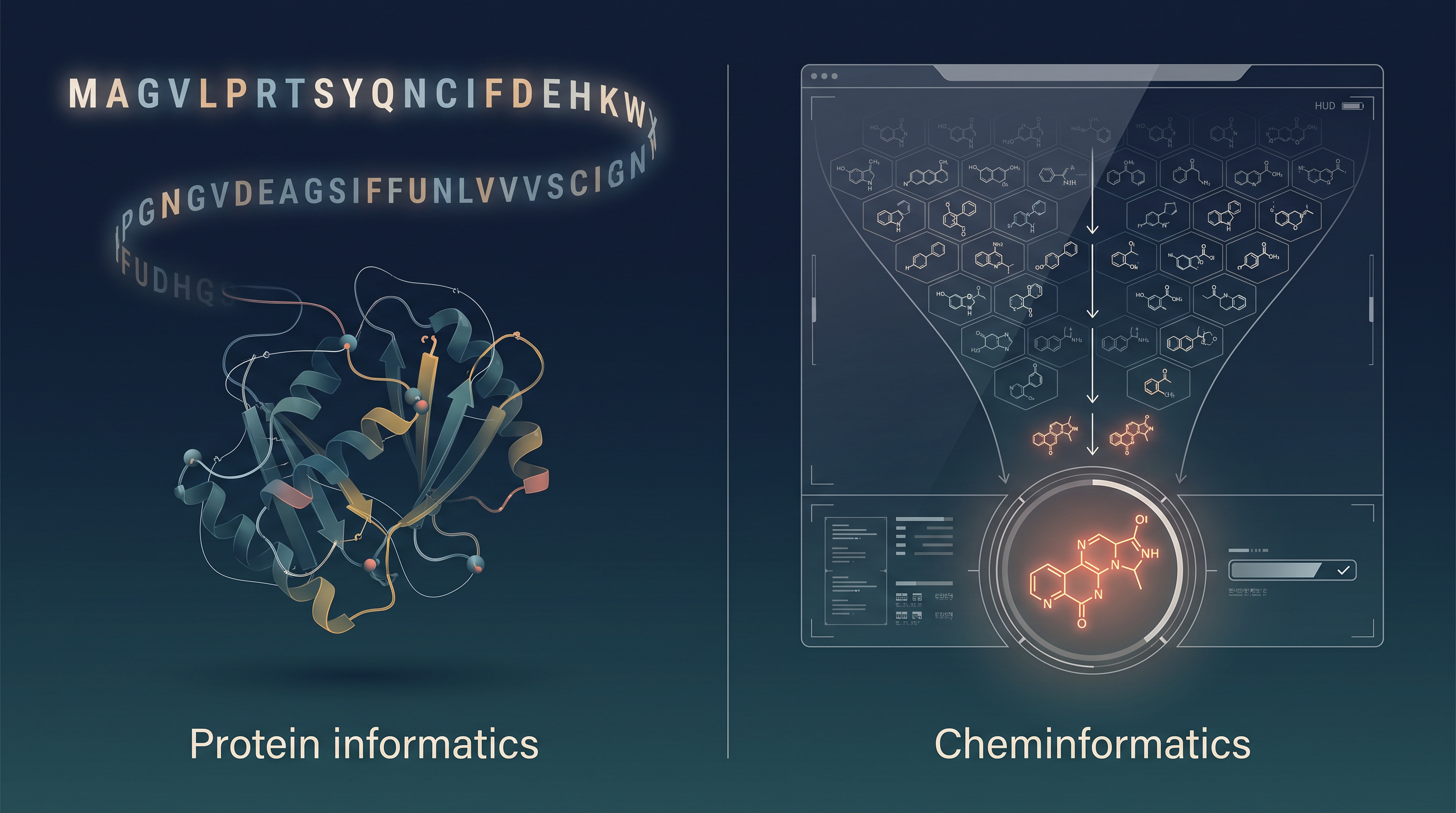
Fig. 10.0

Fig. 10.0 – Protein informatics and cheminformatics.

NoteCuriosity Corner

Q1. If scientists know only the gene sequence and have never held the protein in a test tube, can a computer still predict what that protein looks like? Q2. How can a computer tell, before the protein is ever purified, whether it will be acidic or basic, and whether it will stay stable in a test tube? Q3. Why do chemists store molecules inside computers as graphs of nodes and edges instead of simply saving a picture of the structure? Q4. Out of billions of possible compounds, how does a computer shortlist the handful that might become a successful oral medicine? Q5. What exactly is a pharmacophore, if it is not a molecule at all?

By the end of this chapter, you will be able to answer each of these questions yourself.

10.1 Protein Informatics

10.1.1 Introduction

Every living cell runs on proteins. Enzymes that speed up reactions, receptors that receive signals, antibodies that recognise invaders, transporters that carry molecules across membranes — all of these are proteins. If we want to understand how a cell works, or design a medicine that acts on it, we must first know what each protein is and what it does.

The difficulty is one of sheer volume. Modern sequencing projects have handed biologists millions of protein sequences, far more than any laboratory could ever purify, crystallise and study one at a time. This is where information technology enters biology.

Collecting information about any protein using the techniques of information technology comes under protein informatics. In simple words, it is the practice of using computers, databases and algorithms to extract meaningful biological knowledge from protein data that has already been generated.

NoteDefinition

Protein informatics is the branch of bioinformatics in which information about a protein is collected, stored, and analysed using the techniques of information technology.

What protein informatics has achieved

Protein informatics has been of tremendous help in three related tasks for hypothetical proteins — proteins whose existence has been inferred from a gene sequence, but which have never actually been isolated or studied in a laboratory.

First, it helps find the geometrical location of the functional site, that is, the exact pocket or groove on the folded protein where a substrate or partner molecule binds. Second, it helps assign the biochemical function — the chemical reaction the protein carries out. Third, it helps assign the biological function — the role that reaction plays in the life of the organism.

A protein can only be understood once we know its shape, so a fourth achievement follows naturally: protein informatics has led to the determination of the tertiary structures of many hypothetical proteins. Tertiary structure is the complete three-dimensional folded shape of a single polypeptide chain, and it is this shape that decides what the protein can bind and what it can do. For many of these proteins, conventional laboratory methods had failed to reveal any molecular function at all.

Q. If a protein has never been isolated, where does the “data” about it come from?

A. From the genome. Once a gene is sequenced, its coding region can be translated on a computer into the amino acid sequence of the protein it would make. That predicted sequence becomes the starting raw data, even though the protein itself has never been seen in a test tube.

The resources that made it possible

Protein informatics did not grow out of clever software alone. It grew because two kinds of resources became available together.

One is heterogeneous databases — collections of very different kinds of information (sequences, structures, images, interaction records, spectra) maintained in different formats and at different centres, which can nevertheless be searched together.

The other is a large set of descriptors. A descriptor is a measurable number or code that stands for some property of a molecule, so that a computer can compare molecules mathematically instead of by eye. Descriptors of amino acid sequences, of tertiary structures, and of pathways on the proteome scale (the proteome being the complete set of proteins expressed by an organism) have all helped protein informatics develop into a working science.

10.1.2 Protein data types

Computation cannot begin from nothing. The process of computation of information extraction needs raw data of protein, and that raw data must first be generated experimentally or derived from a genome. Different experiments produce very different kinds of protein data, and each kind answers a different question.

The eight kinds of raw protein data

The protein data used in protein informatics can be of the following types —

  1. Microscopic image of heat-denatured protein aggregate. When a protein solution is heated, the chains unfold and clump together into an aggregate with a characteristic texture, which is photographed under a microscope.

  2. Protein in solution form. The purified protein dissolved in a buffer, on which physical and chemical measurements can be made directly.

  3. Protein sequence as output of Matrix Assisted Laser Desorption Ionisation (MALDI). MALDI is a mass-spectrometry technique in which the protein sample is embedded in a matrix, blasted with a laser, and the resulting ionised fragments are measured. It reads out short stretches of sequence rather than the whole chain.

  4. Assembled protein sequence. The complete, full-length sequence of amino acids, put together from such shorter reads.

  5. Protein crystal structure in Protein Data Bank (PDB) format. The experimentally determined three-dimensional structure, written as a standard file of atomic coordinates.

  6. Protein-protein, protein-ligand or protein-nucleotide interaction file. A record of which molecule binds which — another protein, a small ligand, or a stretch of DNA or RNA.

  7. Nuclear Magnetic Resonance (NMR) data and Mass Spectrometry (MS) data. NMR reports on the environment of atomic nuclei in a magnetic field and can give structural information for proteins in solution; MS reports very accurate molecular masses.

  8. Protein sequences derived directly from the genomic sequences, which do not contain the known evidence of existence (Hypothetical protein). These are the sequences that a computer has translated from a gene, with no experimental proof yet that the protein is actually made.

Notice how the list moves from the crudest data (a photograph of a clump) to the most abstract (a sequence that exists only inside a computer). Protein informatics is valuable precisely because it can squeeze information out of every one of these.

What each kind of data tells us

The above mentioned types of protein data can be used for getting useful information like —

  1. Multi-fractal property of microscopic image of heat-denatured protein aggregate is used for designing protein-marker. A fractal pattern is one that repeats a similar texture at different magnifications; when a single number cannot describe that texture, several are needed, and the pattern is called multi-fractal. Since different proteins aggregate with different textures, this property can be turned into a marker that identifies a protein.

  2. Protein data in solution are useful for analysing physico-chemical properties and kinetics information. Solution studies tell us how the protein behaves in water — its charge, its solubility, and how fast it catalyses a reaction.

  3. Fragmented short sequences of proteins from MALDI are used to find out the full length sequence. The short pieces overlap, and a computer joins the overlaps to reconstruct the whole chain — much like assembling a torn page from its fragments.

  4. Protein crystal structures are used to study mutations and interactions. Once the atomic positions are known, one can see exactly which residue a mutation would change and whether that residue sits at a binding surface.

  5. PDB, NMR and MS data are also used for the prediction of structure of non-crystallised protein (directly from the sequence). Many proteins simply refuse to crystallise. Existing structures then serve as templates from which the shape of the uncrystallised protein is predicted.

  6. There are proteins which do not have known existences (hypothetical proteins) which can be identified from the genomic sequences.

  7. Network mapping of protein provides information about the possible target of treatment of different diseases. A network map shows which protein influences which, so a researcher can identify the one node whose blocking would shut down a disease pathway.

In the early 1970s, a small archive of protein structures was set up at Brookhaven National Laboratory in the United States. It began with only a handful of structures solved by X-ray crystallography. That archive was the Protein Data Bank, and it has since grown into the central worldwide repository of experimentally determined biomolecular structures — the resource without which none of the modern structure-prediction methods described in this chapter could work. Its founding established a habit that biology has followed ever since: solve a structure, then deposit it where everyone can use it.

What a protein informatics laboratory needs

In order to carry out the protein informatics analysis, the following two basic facilities are required.

  1. Availability of the raw data from various databases, such as NCBI, PDB, CHEMBL, BIOMODELS, etc. Without free access to deposited data, every laboratory would have to generate its own, and computation would lose its main advantage.

  2. Informatics tools and techniques used for the analyses. Some of the well known techniques are: (a) image analysis by the wavelet techniques, (b) sequence similarity and homology calculations, (c) structure optimisation techniques, (d) data analysis by statistical and machine learning techniques as Artificial Neural Network (ANN), Support Vector Machine (SVM) and Hidden Markov Model (HMM), (e) Network Mapping Technique, and (f) Systems Biology Mark-up Language (SBML).

Each of these has a clear job. Wavelet techniques break an image into patterns at several scales, which is why they suit the fractal textures of protein aggregates. Sequence similarity and homology calculations measure how alike two sequences are, and are the basis of every template-based prediction. Structure optimisation adjusts a rough model until its atoms sit at energetically sensible distances. ANN, SVM and HMM are machine-learning methods that learn rules from thousands of known examples and then apply those rules to a new, unknown protein. Network mapping builds the protein interaction maps described above, and SBML is a standard computer language for writing biological models so that different laboratories’ models can be exchanged and combined.

Q. Why do these methods need such large databases of known proteins?

A. Because every one of them works by comparison. A machine-learning method can only recognise a pattern it has been shown before, and a homology calculation can only succeed if a similar sequence with a known structure already exists. The bigger and better-curated the database, the more reliable the prediction.

10.1.3 Computational prediction of protein structures

Protein structure prediction using bioinformatics tools is aimed to explore how amino acid sequences specify the structure of proteins, and how these proteins bind to substrates and other molecules to perform their functions. It is, in other words, an attempt to read shape and function out of sequence.

The most striking feature of this task is when it becomes possible. Predicting the structure of a protein — including those of hypothetical proteins — using bioinformatics tools is possible even when only the gene sequence is known, that is, in the absence of the protein sequence itself. The gene is translated on the computer into a sequence, and prediction proceeds from there.

Many computational tools are available from different sources for making predictions of structural and physico-chemical properties of proteins. The major advantages of computational methods are the time frame involved, the low cost, and the feasibility of high throughput screening — that is, the ability to run the same analysis on thousands of proteins one after another without any extra laboratory work.

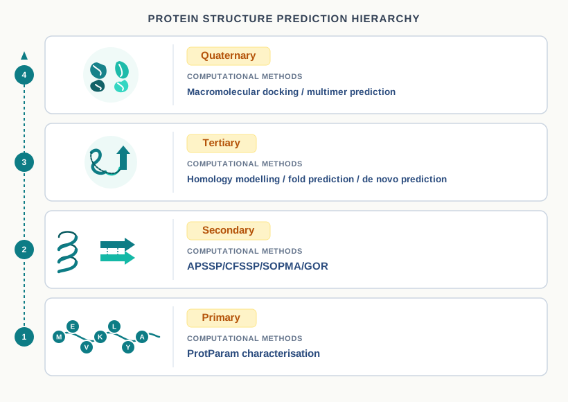
It helps to remember that prediction follows the natural hierarchy of protein structure, as shown in Fig. 10.1. The primary structure is the sequence of amino acids; the secondary structure consists of local regular folds such as α-helices and β-pleated sheets; the tertiary structure is the full three-dimensional shape of the chain. Prediction climbs this ladder one rung at a time, because each level constrains the next.

Fig. 10.1

Fig. 10.1 – Levels of protein structure and their prediction methods.

Q1. If scientists know only the gene sequence and have never held the protein in a test tube, can a computer still predict what that protein looks like?

A. Yes. The gene sequence is translated on the computer into the amino acid sequence, and structure prediction tools work from that sequence alone. This is exactly how the structures of hypothetical proteins — proteins with no experimental evidence of existence — are obtained, at a fraction of the time and cost of laboratory methods.

10.1.3.1 Primary structure prediction

Protein primary structure prediction involves physico-chemical characterisation such as isoelectric point, extinction co-efficient, instability index, aliphatic index and grand average hydropathy. All these can be calculated with the help of the ProtParam tool of the ExPASy Proteomics Server. Some of the physico-chemical properties of proteins are described in brief below.

These numbers matter for very practical reasons. Before a protein is ever expressed and purified, they tell a researcher what buffer to use, whether the protein will survive in a test tube, and whether it is likely to be soluble in water.

ProtParam physico-chemical characterisation of primary structure Principle: Every physico-chemical property of a protein is decided by the identity and order of its amino acids; therefore each property can be computed from the sequence alone using known values for the individual residues. Steps: Obtain the amino acid sequence (experimentally, or by translating the gene) → paste the sequence into the ProtParam tool of the ExPASy Proteomics Server → the tool computes isoelectric point, extinction co-efficient, instability index, aliphatic index and grand average hydropathy → interpret each value against its standard cut-off. Used for: Planning purification and storage before any wet-lab work — for example, choosing the pH of the buffer for isoelectric focusing, or predicting whether a recombinant protein will be stable enough to handle.

Isoelectric point — Isoelectric point (pI) is the pH at which the surface of protein is covered with charge but net charge of protein is zero. The surface still carries plenty of positive and negative groups; they simply cancel out exactly. At pI, proteins are stable and compact, because there is no overall charge to make different parts of the molecule repel one another.

If the computed pI value is less than 7 (pI<7), it indicates that protein is considered as acidic. The pI greater than 7 (pI>7) reveals that protein is basic in character. The computed isoelectric point will be useful for developing the buffer system for purification by the isoelectric focusing method, in which proteins migrate through a pH gradient and each one stops moving exactly at the pH equal to its own pI.

NoteDefinition

The isoelectric point (pI) of a protein is the pH at which its surface is covered with charge but its net charge is zero; at this pH the protein is stable and compact. A pI below 7 indicates an acidic protein and a pI above 7 a basic protein.

The aliphatic index — The aliphatic index (AI) is defined as the relative volume of a protein occupied by aliphatic side chains (A, V, I and L). These one-letter symbols stand for alanine, valine, isoleucine and leucine, the amino acids whose side chains are simple hydrocarbon chains. The aliphatic index is regarded as a positive factor for the increase of thermal stability of globular proteins, because these bulky non-polar side chains pack tightly into the protein’s core and hold the fold together when heat tries to shake it apart. Very high aliphatic index of protein sequences indicates that protein may be stable for a wide temperature range.

NoteDefinition

The aliphatic index (AI) is the relative volume of a protein occupied by its aliphatic side chains (A, V, I and L); a high value indicates greater thermal stability of a globular protein over a wide temperature range.

The instability index — The instability index provides an estimate of the stability of protein in a test tube. It is built on a simple observation: there are certain dipeptides — particular pairs of neighbouring amino acids — the occurrence of which is significantly different in the unstable proteins compared with those in the stable ones. This method assigns a weight value of instability to each such dipeptide. Using these weight values it is possible to compute an instability index for the whole sequence.

A protein whose instability index is smaller than 40 is predicted as stable; a value above 40 predicts that the protein may be unstable. This single cut-off is worth memorising, since it is a favourite of assertion–reason and data-interpretation questions.

NoteDefinition

The instability index estimates the stability of a protein in a test tube from the weight values of destabilising dipeptides present in its sequence; a value below 40 predicts a stable protein, while a value above 40 predicts an unstable one.

The Grand Average Hydropathy (GRAVY) value — The Grand Average Hydropathy value for a peptide or protein is calculated as the sum of hydropathy values of all the amino acids, divided by the number of residues in the sequence.

\[\mathrm{GRAVY} = \frac{\displaystyle\sum_{i=1}^{n} h_i}{n}\]

Here \(h_i\) is the hydropathy value of the \(i\)-th amino acid residue (a dimensionless number that is positive for water-repelling residues and negative for water-attracting ones), and \(n\) is the total number of residues in the sequence. GRAVY itself is dimensionless, since it is an average of dimensionless values.

The low range of GRAVY value indicates the possibility of better interaction with water. That makes sense: a low average hydropathy means the chain is dominated by residues that prefer water, so the protein is likely to be soluble rather than buried in a membrane.

A short recombinant peptide is 25 residues long. The hydropathy values of its residues add up to \(-11.5\). Calculate its GRAVY value, and state whether the peptide is more likely to be soluble in water or to sit inside a lipid membrane. Justify your answer.

Q2. How can a computer tell, before the protein is ever purified, whether it will be acidic or basic, and whether it will stay stable in a test tube?

A. From the sequence alone. The isoelectric point computed by ProtParam decides acidic (pI<7) or basic (pI>7) character, while the instability index decides test-tube stability — below 40 the protein is predicted stable, above 40 unstable. The aliphatic index adds a prediction about stability across a range of temperatures.

10.1.3.2 Secondary Structure Prediction

The protein secondary structure has been studied intensely, since it is very helpful to reveal the functions of protein with unknown structures. Secondary structure describes the local, regularly repeating folds of the backbone — chiefly α-helices and β-pleated sheets — and the pattern in which these elements occur along a chain is often characteristic of a particular family of proteins.

In addition, it has been shown that the prediction of protein secondary structure is a step towards protein 3-dimensional structure prediction. This is the reason secondary structure prediction is never treated as an end in itself: knowing which stretches form helices and which form sheets massively reduces the number of three-dimensional arrangements a program must consider later.

APSSP, CFSSP, SOPMA, and GOR are common protein secondary structure prediction tools. Each takes an amino acid sequence as input and returns, for every residue, whether it is predicted to lie in a helix, a sheet, or a coil.

10.1.3.3 Three dimensional (3D) Structure Prediction

The following three computational methods are commonly used to predict protein 3D structure. They differ mainly in how much they lean on structures that are already known.

Homology modelling — For homology modelling, the amino acid sequence of a protein with unknown structure is aligned against sequences of proteins with known structures. High degrees of homology — that is, very similar sequences across and between the proteins — can be used to determine the global structure of the protein with unknown structure and place it into a certain fold category.

Lower degrees of homology may still be used to determine the local structures, an example being the Chou-Fasman method for predicting secondary structure. An advantage of homology modelling methods is lack of dependence on the knowledge of physical determinants; the method does not need to calculate the forces that make the protein fold, because it borrows a shape that nature has already been shown to adopt. MODELLER and SWISS-MODEL are commonly used tools for homology modelling.

Homology modelling Principle: Proteins with similar amino acid sequences fold into similar three-dimensional shapes, so a known structure can serve as a template for an unknown one. Steps: Take the sequence of the unknown protein → search the databases for homologous sequences whose structures are already known → align the unknown sequence with the template sequence → build a model by placing the unknown protein’s residues on the template’s backbone → refine the model. Used for: Rapidly obtaining a working 3D model of a protein that has not been crystallised, using tools such as MODELLER and SWISS-MODEL.

Fold prediction — With the method called ‘threading’, the sequence of a protein with unknown structure is forced to take the conformation of the backbone (protein side chains) of a protein with known structure. The sequence is, in effect, threaded through one candidate fold after another and scored for how comfortably it fits. These methods tend to be more compute-intensive than homology modelling methods, but they give more confidence in the physical viability of the results, because the fit is judged on physical grounds rather than on sequence similarity alone. LIBELLULA and Threader are commonly used tools for this method.

De novo protein structure prediction — It is an algorithmic process by which protein tertiary structure is predicted from its amino acid primary sequence. Here nothing is borrowed at all: the model is built from first principles, which is why the approach is also called ab initio (meaning “from the beginning”). QUARK is a computer algorithm for ab initio protein structure prediction and protein peptide folding, which aims to construct the correct protein 3D model from amino acid sequence only.

Homology modelling vs Fold prediction (threading) vs De novo prediction | Feature | Homology modelling | Fold prediction (threading) | De novo prediction | |—|—|—|—| | Basis of the method | Sequence similarity to a protein of known structure | Fitting the sequence onto known backbone conformations | Building the structure from the amino acid sequence alone | | Template required | Yes, a homologous structure | Yes, a library of known folds | No | | Computing demand | Lowest of the three | More compute-intensive than homology modelling | Highest | | Main strength | Fast; independent of knowledge of physical determinants | Greater confidence in physical viability of the result | Works even when no related structure exists | | Common tools | MODELLER, SWISS-MODEL | LIBELLULA, Threader | QUARK |

Q. If homology modelling is faster and easier, why bother with threading or de novo methods at all?

A. Because homology modelling fails when no relative of the protein has a known structure. Threading can still recognise a suitable fold even when the sequences are not obviously similar, and de novo methods can attempt a structure when neither a homologue nor a matching fold is available. The three methods form a sequence of fall-backs, not a set of rivals.

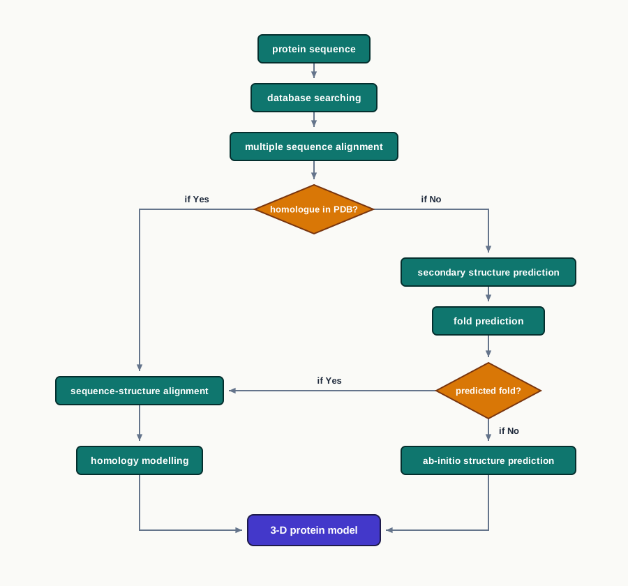
The choice between them is not made at random. The complete decision path, from a raw protein sequence to a finished 3D model, is summarised in Fig. 10.2: the sequence is first searched against the databases, and only if no homologue is found in PDB does the analysis fall back on secondary structure prediction, fold prediction, and finally ab initio modelling.

Fig. 10.2

Fig. 10.2 – Routes for protein structure prediction.

How a predicted structure is stored

A structure is of no use to anyone else unless it can be shared in a standard form. Computationally elucidated structure of a protein is recorded as atomic coordinates in protein-data-bank files. The three-dimensional coordinates are stored in a type of text-file namely PDB-file with file extension .pdb in the Protein Data Bank (PDB) database. It contains data from X-ray crystallography, NMR and a few theoretical structure models.

The coordinates are simply the \(x\), \(y\) and \(z\) positions of every atom, so a PDB file is a plain list of numbers that any visualisation program anywhere in the world can read and redraw as a ribbon or space-filling model.

Domain prediction

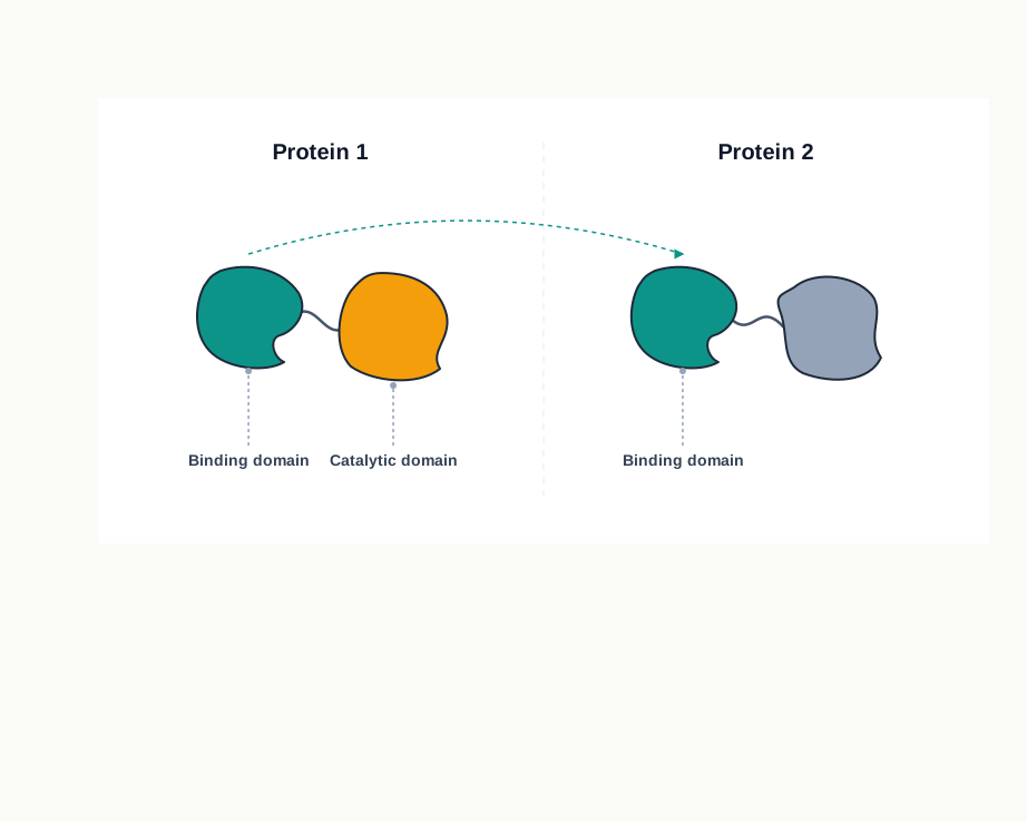
A domain is a distinct functional and/or structural unit of a protein. An independent folding unit of a polypeptide chain also carries specific function. Domains are often identified as recurring (sequence or structure) units, which may exist in various contexts — the same domain may turn up in several unrelated proteins, each time bringing the same function with it, as shown in Fig. 10.3.

Fig. 10.3

Fig. 10.3 – Recurring protein domains.

NoteDefinition

A domain is a distinct structural and/or functional unit of a protein that folds independently of the rest of the polypeptide chain and carries a specific function; the same domain may recur in different proteins.

The most common tools for domain prediction are InterPRO scan of EMBL and CDD search of NCBI. Both work by comparing the query sequence against a curated library of domain signatures and reporting every match, together with the region of the sequence in which it lies.

Q. A newly sequenced bacterial genome yields a hypothetical protein of unknown function. What is the quickest computational step to guess what it does?

A. Run a domain search. If the sequence contains a recognised domain — say an ATP-binding domain or a DNA-binding domain — the protein’s likely biochemical role is suggested at once, and this guess can then guide the structure prediction and the eventual laboratory test.

10.2 Cheminformatics

10.2.1 Introduction

The previous section dealt with the biological half of a drug’s story — the protein that a medicine must act upon. This section deals with the chemical half: the molecule that will act on it. Once a target protein has been identified, someone must find, out of an enormous number of possible compounds, the one that binds it correctly.

The use of computational and informational techniques to understand problems of chemistry is known as cheminformatics. This is an interface science, combining principles of physics, chemistry, biology, mathematics, biochemistry, statistics and informatics. Terms like chemoinformatics and chemical informatics are used along with cheminformatics, to indicate the same approach.

NoteDefinition

Cheminformatics is the use of computational and informational techniques to solve problems of chemistry, drawing on physics, chemistry, biology, mathematics, biochemistry, statistics and informatics. Chemoinformatics and chemical informatics are alternative names for the same approach.

Cheminformatics strategies are useful in drug discovery, where a large number of compounds are evaluated for interaction with the target cellular molecules. Evaluating them one by one in a laboratory would be impossibly slow and expensive; evaluating them inside a computer is neither.

Where cheminformatics is used

For the last two decades, the science of cheminformatics has grown conceptually and technically, finding widespread applications in chemical industry, pharmaceutical and biotechnology research — for example, in computer-aided drug design (CADD), where one looks for molecules with specific biological and therapeutic properties.

Cheminformatics specialists handle information on physical properties, three-dimensional molecular and crystal structures, chemical reaction pathways and so on. In addition to real compounds, cheminformatics researchers primarily handle virtual libraries of chemical databases that can contain hypothetical compounds.

A virtual library is a collection of molecules that exist as data rather than as substances in a bottle. Virtual libraries can contain information on likely synthesis methods and predicted stability of the reaction products, so a researcher can judge in advance whether a compound is worth making at all.

Virtual screening uses chemical and physical principles to identify and evaluate the best candidates for a particular property or reaction from large libraries of real and virtual molecules. The most desirable candidates can then be verified in laboratory studies. Notice the division of labour: the computer eliminates, the laboratory confirms.

Q. Why is it useful to store molecules that have never been made?

A. Because the cost of testing a molecule in a computer is almost nothing, while the cost of synthesising it is very high. If the computer predicts that a hypothetical compound would bind the target well and could realistically be synthesised, only then is it worth a chemist’s time. Virtual libraries let researchers explore chemical possibilities far beyond what has actually been made.

10.2.2 Storing and managing the chemical data

Many groups and organisations maintain databases of chemical compounds. Some of them are publicly available for free and some of them are commercially available. Though these databases contain millions of chemical compounds, their reactions and so on, the computational power and tools are so robust that it takes only a few seconds to search through the entire resource and retrieve the records.

Science has advanced so much that we have libraries of virtual molecules running into billions of entries — these are compounds that do not exist according to the available literature, but can be synthesised using advanced combinatorial techniques, in which a set of chemical building blocks is combined in every possible arrangement to generate a very large family of related molecules.

The CAS registry

CAS (Chemical Abstracts Service), a division of the American Chemical Society, is the world’s largest collection of chemistry insights. It is an authoritative source of chemical names and structures, and serves as a universal standard for chemists — which matters greatly, because the same molecule may be written in several different ways by different laboratories.

At present, the CAS registry hosts more than 219 million organic and inorganic substances taken from literature. The registry includes more than 70 million protein and nucleic acid sequences. The database contains more than 8 billion property values of substances.

Data from a large number of globally published literature — including biomedical sciences, chemistry, engineering, material science and so on — are added to the CAS database every day. This tremendous resource is a treasure for finding compounds of therapeutic and industrial importance.

Some of the popular chemical databases are mentioned in Table 10.1. Read the table not as a list to be memorised but as a map: each database was built to answer a different kind of question, and choosing the right one is the first skill of a cheminformatics worker.

Table 10.1: Popular Chemical Database

Name Description
PubChem PubChem is a database of chemical molecules which maintains three types of information namely, substance, compound and BioAssays.
ZINC ZINC database contains a large number of compounds available for virtual screening. In this database, various molecule features like molecular weight, log P etc. are included.
ChEMBL This database provides comprehensive information on a large number of bioactive (small drug-like molecules) compounds with drug targets.
NCI NCI database has a large number of small molecule structures, a very useful resource for researchers working in the field of cancer/AIDS.
ChemDB It is a database of chemicals containing information of chemicals, which includes predicted or experimentally determined physicochemical properties, such as 3D structure, melting temperature, and solubility.
ChemSpider ChemSpider contains unique chemical entities aggregated from diverse data sources.
BindingDB It is a binding affinity database of small molecules for their protein targets.
DrugBank The database that combines detailed drug (i.e., chemical, pharmacological and pharmaceutical) data with comprehensive drug target (i.e., sequence, structure, and pathway) information.
PharmaGKB It is a pharmacogenomics knowledge resource that encompasses clinical information of drug molecules.
SuperDrug This database contains 3D-structures of active ingredients of essential marketed drugs.

10.2.3 Why do we need cheminformatics?

Faced with hundreds of millions of compounds, properties, chemical reactions and so on, the question is how to navigate this huge resource and find the right chemical compound that meets our requirements.

The cheminformatics tools help us browse through the enormous body of literature and find patterns. A pattern here might be a shared structural feature among all the compounds that are active against a particular target — the kind of regularity a human reader would never notice across a million records.

Pharma companies use cheminformatics resources and tools for in silico design of novel drugs, followed by synthesis and testing. The phrase in silico means “in silicon”, that is, inside a computer, and is used alongside the older terms in vivo (in a living organism) and in vitro (in glassware).

The chemical manufacturing industry needs cheminformatics to design new properties, and to predict the efficacy and toxicity of chemicals before they reach the market. Predicting toxicity early is not only cheaper — it prevents harmful compounds from ever being made in bulk.

10.2.4 How to store information on chemical compounds?

One can easily draw chemical compounds on paper, with bonds in between the atoms and aligned at a certain angle. Using drawing tools, it is possible to use predefined templates on the user interface and draw standard geometric structures and reactions with ease. One can store such information as an image file (e.g., jpg, tif) or in document form (e.g., doc, pdf).

However, such a storage of chemical data is of little use in research projects that demand ‘deep browsing’ into bond angles, flexibility of rotation and so on, to find the right molecule for a particular purpose. The reason is simple: a picture is only a pattern of coloured dots to a computer. It cannot be asked which atom is joined to which, or how freely a bond can rotate.

Molecules as graphs

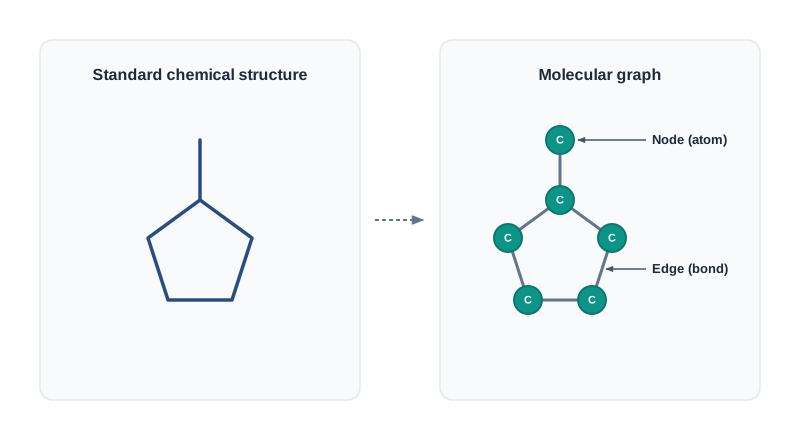
Chemical structures are therefore stored in the computer as molecular graphs. A graph is an imaginary representation of nodes (units of chemical substances) and edges (movement of information between nodes). Using the node-edge approach, one can create graphs representing atoms and bonds, as shown in Fig. 10.4.

Fig. 10.4

Fig. 10.4 – Chemical structure and its molecular graph.

Once a molecule is a graph, a computer can do genuine chemistry with it — count rings, trace paths, and compare one structure with another mathematically rather than visually.

At a higher level, the same representation is used to build molecular pathways in the cell, for example glycolysis and Kreb’s cycle. Here the nodes are metabolites and the edges are the enzymatic conversions between them, which is why a single computational idea serves both a single molecule and an entire metabolic map.

NoteDefinition

A molecular graph is a computer representation of a chemical structure in which nodes stand for units of chemical substances (atoms) and edges stand for the connections between them (bonds).

Q3. Why do chemists store molecules inside computers as graphs of nodes and edges instead of simply saving a picture of the structure?

A. Because an image file stores only the appearance of a structure, not its chemistry. A molecular graph stores the actual connectivity — which atom is bonded to which — so the computer can search for substructures, examine bond angles and rotational flexibility, and compare millions of molecules automatically. The same node-and-edge idea also scales up to represent whole metabolic pathways such as glycolysis.

10.2.5 Searching the structures

It is common for commercially available databases to have their origins in academic research projects. This is true for cheminformatics as well.

The simplest task is to extract information about chemical structure. For example, if you are interested in discovering the physical and chemical properties of a substance, the database can provide you with information on all the chemical substances that fall within a specific boiling point range, and more.

Substructure retrieval

Another aspect of the search process is substructure retrieval. For example, it displays the various chemical compounds associated with specific functional groups, such as a methyl group, benzene ring, or alkene backbone. This is exactly the search a medicinal chemist needs, because biological activity often depends on the presence of one particular chemical grouping.

We refer to the complete embedding of a small graph into a larger one as subgraph isomorphism (iso, meaning multiple forms of the same type). In plain terms, the computer asks whether the pattern of nodes and edges you have drawn can be found, unchanged, somewhere inside the bigger molecular graph.

NoteDefinition

Subgraph isomorphism is the complete embedding of a smaller graph within a larger one — the computational basis on which a substructure is recognised inside a molecule.

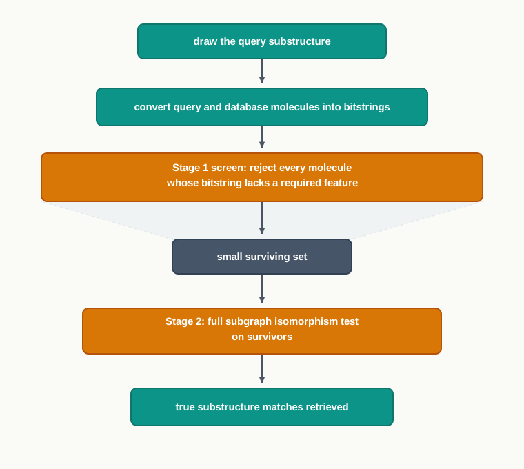
Testing this for every molecule in a database of hundreds of millions would be far too slow, because subgraph isomorphism is a computationally heavy operation. For this reason, people often perform a two-stage search.

The first stage or step involves filtering out molecules that may not be a potential match for the substructure query. During this stage, we eliminate most of the molecules, leaving behind a small fraction that may be worth further investigating in the next stage.

The second stage or step involves a more elaborate subgraph isomerism process to find molecules that truly match a given substructure. Only the survivors of stage one are put through this expensive test, which is why the two-stage design saves so much time. The full sequence is summarised in Fig. 10.5.

We implement molecule screens using binary strings of 0s and 1s, known as bitstrings. Each position in the bitstring records the presence (1) or absence (0) of one particular structural feature, so two molecules can be compared almost instantly by comparing their strings — and any molecule lacking a feature that the query demands can be rejected without further examination.

Fig. 10.5

Fig. 10.5 – Two-stage substructure search.

Substructure search Principle: A molecule contains a given substructure only if the small query graph can be completely embedded within the larger molecular graph (subgraph isomorphism). Steps: Represent every molecule as a molecular graph → encode structural features as bitstrings → Stage 1, screen the database with bitstrings to eliminate impossible matches → Stage 2, apply the full subgraph isomorphism test to the small surviving set → return the matching compounds. Used for: Retrieving every compound in a database that carries a particular functional group — for instance, listing all available molecules containing a benzene ring when designing a new drug series.

Q. Why not simply run the accurate subgraph isomorphism test on the whole database and skip stage one?

A. Because it would take far too long. The accurate test is computationally expensive, and most molecules in the database are obviously wrong. The bitstring screen throws those out in a fraction of a second, so the expensive test is run only on the few molecules that could possibly match. The answer is the same; only the time taken is different.

10.2.6 Searching the reactions

Structures are not the only thing worth searching. While planning a synthesis, a chemist may wish to search the reaction database for products, to find if someone has already synthesised a given compound and, if yes, what the reaction conditions were.

Also, one may want to know how many different reaction pathways exist to move from point A to point X in the pathway. Further, one may need information on solvents, pH, temperature, pressure and so on. A route that works only at high pressure may be useless to a laboratory that has no such equipment, so conditions matter as much as the reaction itself.

One can refine reaction queries by integrating several queries into one statement: find all reactions that utilise glucose and operate within temperature range of 37°C. This single query combines a reactant condition and a temperature condition, and returns only the reactions satisfying both.

A key feature of reaction search is atom mapping, that is, finding an exact correspondence between reactant atoms and the resultant products. Atom mapping tells the chemist which atom in the product came from which atom in the reactant, which is essential for understanding the mechanism and for designing labelling experiments. The existing cheminformatics tools and databases also allow retrieval of reactions where a certain substructure is converted into products.

10.2.7 Pharmacophore

A pharmacophore is a description of molecular features that define molecular recognition of a ligand. A ligand, here, is any small molecule that binds specifically to a larger target molecule such as a receptor protein.

The IUPAC defines pharmacophore as an ensemble of steric and electronic features necessary to ensure optimal interactions with a specific biological target and trigger a biological response. Steric features concern shape and size — what fits into the binding pocket. Electronic features concern charge and polarity — what attracts and what repels once it is inside.

NoteDefinition

A pharmacophore is an ensemble of the steric and electronic features of a molecule that are necessary to ensure optimal interaction with a specific biological target and to trigger a biological response.

A pharmacophore model explains how structurally diverse ligands can dock on to a single receptor molecule. This is an important insight: two molecules that look quite different on paper can still act on the same receptor, provided they both carry the required features in the required spatial arrangement.

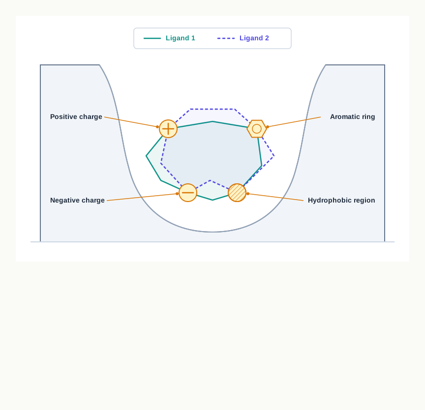
A 3D pharmacophore is a set of features related to spatial orientation, for example positively and negatively charged groups, rings and hydrophobic regions, as illustrated in Fig. 10.6. What the receptor “sees” is not the whole molecule but this arrangement of features in space.

Fig. 10.6

Fig. 10.6 – Pharmacophore features of two different ligands.

It is important to know that a pharmacophore is not a physical molecule or a group of molecules. It cannot be weighed, bottled, or synthesised. The pharmacophore is a well established conceptual framework that defines a specific molecular description — pharmacophore points such as steric, electrostatic and hydrophobic properties — of a therapeutic molecule needed for its interaction with a target.

Pharmacophore modelling Principle: Binding to a target depends not on the whole molecule but on a particular set of steric and electronic features arranged correctly in three-dimensional space. Steps: Collect molecules known to be active at the target → identify the chemical features they share (charged groups, rings, hydrophobic regions) → determine the spatial arrangement of these features → build a 3D pharmacophore model → search chemical databases for other molecules that match the model. Used for: Finding structurally new drug candidates that act on a known receptor, and as one of the ligand-based filters in virtual screening.

Q5. What exactly is a pharmacophore, if it is not a molecule at all?

A. It is a description, not a substance — the ensemble of steric and electronic features, arranged in a particular way in space, that a molecule must possess to bind a given target and trigger a biological response. Because it describes features rather than a specific structure, chemically very different ligands can satisfy the same pharmacophore and dock on to the same receptor.

10.2.8 Lipinski’s rule of five (R05)

This rule was proposed by Christopher A. Lipinski in 1997 and describes the key molecular properties of compounds. It came from a practical frustration: many compounds that bound their target beautifully in a test tube failed as medicines because they were never properly absorbed after being swallowed.

Ideally, a drug should be biodegradable, non-toxic, stable, with no side effects, have uniform cellular distribution, controllable release in the body, be cost-effective and be easily excreted after action. No real drug satisfies all of these perfectly, but they describe the target a designer aims at.

The four criteria

Lipinski’s rule of five includes the following criteria for finding an orally active drug, and the compound should not bear more than one violation.

  1. Not more than 5 hydrogen bond donors
  2. Not more than 10 hydrogen bond acceptors
  3. Molecular weight below 500 Daltons
  4. Octanol water partition coefficient log P of less than 5

Each criterion has a physical reason behind it. To reach the bloodstream from the gut, a molecule must pass through a lipid membrane. Too many hydrogen bond donors or acceptors means the molecule clings to water and will not cross that membrane. Too large a molecular weight means it cannot slip through at all.

The last criterion needs a little unpacking. The partition coefficient \(P\) is measured by shaking a compound between octanol (standing in for the lipid membrane) and water, and comparing the concentrations it settles at in the two layers:

\[\log P = \log_{10}\left(\frac{C_{\text{octanol}}}{C_{\text{water}}}\right)\]

where \(C_{\text{octanol}}\) and \(C_{\text{water}}\) are the equilibrium concentrations of the compound in the octanol and water layers respectively (both in mol L\(^{-1}\)). Since it is a ratio of two concentrations, \(\log P\) is dimensionless. A high \(\log P\) means the compound prefers fat to water; if it is too high, the drug dissolves poorly in body fluids and tends to lodge in fatty tissue instead of reaching its target.

NoteDefinition

Lipinski’s rule of five states that a compound is likely to be an orally active drug if it has not more than 5 hydrogen bond donors, not more than 10 hydrogen bond acceptors, a molecular weight below 500 Daltons, and an octanol–water partition coefficient log P of less than 5, with not more than one violation of these criteria.

What the rule does and does not cover

It is important to remember that Lipinski’s rule of five only deals with finding a chemical compound that has the potential to be a successful oral drug. The RO5 may not apply to drugs given through intramuscular and intravenous routes, because an injected drug bypasses the gut wall entirely and never faces the absorption barrier the rule was written for.

Based on the RO5, the predicted chemical compound is assigned a value between 0–4. The chemical compound having a value less than 3 is not suitable for further analysis. The RO5 does not apply to natural products and semi-synthetic natural products, many of which are large, complex molecules that break the rules and are nevertheless effective medicines.

A candidate compound has a molecular weight of 486 Daltons, 4 hydrogen bond donors, 11 hydrogen bond acceptors and a log P value of 3.8. State how many of Lipinski’s four criteria it violates, and comment on whether it can still be considered a promising orally active drug candidate.

Q. A plant-derived anticancer compound has a molecular weight well above 500 Daltons. Should it be rejected straight away?

A. No. The rule expressly does not apply to natural products and semi-synthetic natural products. Several important medicines derived from plants and microbes break more than one of Lipinski’s criteria and still work, because they are absorbed by routes the rule does not describe or are given by injection. The RO5 is a filter for narrowing down synthetic candidates, not a law of nature.

10.2.9 The journey of a drug

Nature provides an immense storehouse of active compounds with therapeutic applications. Using scientific methods, we have learnt how to narrow down to a certain set of compounds that might make the promising molecules one is looking for. The road to drug discovery and development, however, is long, expensive and risky.

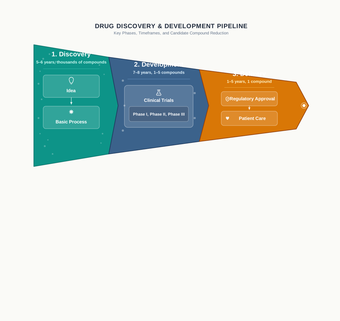
Fig. 10.7 depicts the overall drug discovery pipeline, that is, from lab to the market. The Discovery stage takes about 5–6 years and begins with thousands of compounds, moving from an idea through the basic process. The Development stage takes about 7–8 years, by which time only 1–5 compounds remain, and covers clinical trials in Phase I, Phase II and Phase III. The Delivery stage takes 1–5 years and ends with a single compound passing regulatory approval and reaching patient care.

Fig. 10.7

Fig. 10.7 – Drug development pipeline.

Read the figure as a funnel rather than a road. Thousands of compounds enter at the left and one emerges at the right, after roughly thirteen to nineteen years in total. Every compound eliminated late in this pipeline has already cost a great deal of money — which is precisely why so much effort goes into eliminating the wrong ones early, inside a computer.

Virtual screening

Virtual screening is an in silico approach to decide which compound among billions is useful for a particular purpose. The purpose may be related to drug discovery, industrial applications and so on.

In virtual screening, one scores, ranks and extracts a set of structures using computational methods. The virtual screening may consist of a series of filters that eliminate undesirable compounds at every step.

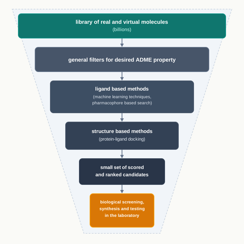
As we move from the first step of virtual screening to the last step, the criteria get increasingly stringent — that is, one moves from a broad set of parameters to a narrow set, with the hope of identifying a small group of molecules that exhibits the desired property. The order matters: the cheap, fast filters are applied first to the largest number of molecules, and the slow, detailed calculations are saved for the few that survive. The sequence is summarised in Fig. 10.8.

Fig. 10.8

Fig. 10.8 – Virtual screening funnel.

Virtual screening may include the use of:

  1. General filters to identify drug-like compounds with a desired Absorption, Distribution, Metabolism and Excretion (ADME) property. ADME describes what the body does to the drug — how it is taken in, spread around, chemically altered and finally removed. Lipinski’s rule of five is a filter of exactly this kind.

  2. Ligand based methods, that encompass machine learning techniques and pharmacophore based search. These methods use knowledge of molecules already known to be active, without needing the structure of the target.

  3. Structure based methods, that include protein-ligand docking. Docking places a candidate molecule into the binding site of the target protein in the computer, tries many orientations, and scores how well it fits. This is where the work of the previous section returns: a docking study needs the 3D structure of the target protein, which may itself have been obtained by homology modelling.

Once a compound passes through these filters, one can use them for biological screening, synthesis, testing and so on.

Ligand based methods vs Structure based methods | Feature | Ligand based methods | Structure based methods | |—|—|—| | What is required | Molecules already known to be active at the target | The three-dimensional structure of the target protein | | Basis of selection | Similarity of features to known active ligands | Physical fit and interaction within the binding site | | Typical approach | Machine learning techniques, pharmacophore based search | Protein-ligand docking | | Used when | The target structure is unknown or unreliable | A good structure of the target is available |

Virtual screening Principle: Undesirable compounds can be eliminated computationally by applying a series of increasingly stringent filters, so that only a small, promising set ever reaches the laboratory. Steps: Assemble a library of real and virtual molecules → apply general filters for drug-likeness and ADME properties → apply ligand based methods such as pharmacophore search and machine learning → apply structure based methods such as protein-ligand docking → score and rank the survivors → verify the top candidates experimentally. Used for: Narrowing billions of possible compounds down to a handful worth synthesising, in drug discovery and in the search for industrially useful chemicals.

Q4. Out of billions of compounds, how does a computer shortlist the handful that might become a successful oral medicine?

A. By virtual screening — a series of filters that get stricter at every step. Broad drug-likeness filters such as Lipinski’s rule of five and ADME criteria remove most of the library first; ligand based methods such as pharmacophore searching narrow it further; and finally structure based protein-ligand docking scores the remaining molecules against the actual target site. Only the top-ranked survivors are synthesised and tested in the laboratory.

Two accidental discoveries 1. In the early 1990s, Pfizer tested a drug called UK92480, which was expected to relax the blood vessels and treat heart complications. Instead, they found an unexpected side effect on the reproductive system, and developed the drug into a blue pill known as Viagra. 2. Do you know the origin of saccharin, the artificial sweetener that we often use in tea or coffee? The origin of this discovery was accidental. One day in 1879, a Russian chemist, Dr Constantin Fahlberg, was so involved with his work that he forgot about supper until it was quite late, and rushed off for a meal without washing his hands. He broke a piece of bread with unwashed hands and put it in his mouth. It tasted very sweet. At this time he did not suspect much; rather, he washed his mouth and dried his moustache with a napkin. Interestingly, the napkin also tasted sweet. Then he drank water, and that also tasted sweet. Immediately, he sensed the breakthrough of a sweetener coming from coal tar. He dropped his dinner, ran back to the lab and tasted the contents of every beaker. One of them had an impure solution of saccharin. Luckily, there was not any corrosive liquid. He worked on this for months, found a chemical method of making saccharin, started a company, and became rich and globally famous for this breakthrough.

Both stories make the same point from opposite directions. Chance has given chemistry some of its most famous products, but chance cannot be planned for — and that is exactly the gap cheminformatics is meant to fill.

Common terminologies in cheminformatics 1. High Throughput Screening (HTS) — A large scale automated process where millions of compounds are tested for a desired property. 2. Hits — Activity observed during high-throughput screening, generally defined by percent activity of new compounds in comparison to well defined and known compounds. 3. False positive — During screening, one may observe situations where a compound is found active in an assay but may turn out to be inactive towards a certain biological target. 4. Lead compound — A compound that is biologically and pharmacologically active with desired properties, and that can be processed further. 5. Library — An inventory of compounds that fulfil the criteria for screening against specific cellular targets. 6. New Chemical Entity — A novel molecule discovered in the lab that has not yet entered clinical trials. 7. Off target activity — Molecular interactions between chemical compounds and cellular molecules that do not bind the target.

How far should a medicine be trusted to computer prediction? Computational screening removes thousands of unsuitable compounds before any animal or human is involved, which reduces animal testing, lowers cost, and can bring a needed medicine to patients sooner. Against this stands a real limitation: a prediction is only as good as the data it was trained on, and false positives and off target activity are recognised problems. A compound that looks safe in a computer may still be toxic in a body. For this reason, regulators everywhere require that computational results be followed by laboratory testing and by Phase I, II and III clinical trials before approval. The safeguard is the pipeline itself — in silico work is allowed to decide what gets tested, never what gets sold.

10.3 Summary

  1. Protein informatics is a growing field of information technology in which information about any protein is collected using sophisticated techniques. Raw data of proteins, collected through various means, is used to retrieve crucial information about the protein of interest.

  2. Protein raw data comes in many forms — microscopic images of heat-denatured aggregates, protein in solution, MALDI output, assembled sequences, crystal structures in PDB format, interaction files, NMR and MS data, and sequences translated directly from genomes (hypothetical proteins). Each form answers a different question about the protein.

  3. Carrying out protein informatics needs two facilities: free access to raw data in databases such as NCBI, PDB, CHEMBL and BIOMODELS, and informatics tools such as wavelet image analysis, sequence similarity and homology calculations, structure optimisation, machine learning methods (ANN, SVM, HMM), network mapping, and SBML.

  4. Structure prediction is possible even when only the gene sequence is known, and its main advantages are speed, low cost and the feasibility of high throughput screening.

  5. Primary structure of a protein can be analysed using the ProtParam tool of the ExPASy Proteomics Server. Isoelectric point, aliphatic index, instability index and Grand Average Hydropathy (GRAVY) value of a protein are calculated using this server.

  6. The cut-offs matter: pI below 7 indicates an acidic protein and above 7 a basic one; an instability index below 40 predicts a stable protein and above 40 an unstable one; a high aliphatic index indicates thermal stability over a wide temperature range; a low GRAVY value indicates better interaction with water.

  7. Secondary structure of a protein is predicted using APSSP, CFSSP, SOPMA and GOR, and this prediction is itself a step towards predicting the three-dimensional structure.

  8. Homology modelling, fold prediction and de novo protein structure prediction are the common computational methods used to predict protein 3D structure. MODELLER and SWISS-MODEL are used for homology modelling, LIBELLULA and Threader for fold prediction by threading, and QUARK for ab initio prediction.

  9. Predicted and experimental structures are stored as atomic coordinates in .pdb files in the Protein Data Bank, which holds data from X-ray crystallography, NMR and a few theoretical structure models.

  10. A domain is a distinct structural and/or functional unit that folds independently and carries a specific function. Domains are predicted using InterPRO scan of EMBL and CDD search of NCBI, and they provide valuable information for the prediction of protein structure, function, evolution and design.

  11. Cheminformatics combines computational and informational techniques to understand the problems related to chemistry. The information used in cheminformatics includes physical properties, 3-D molecular and crystal structures, chemical reaction pathways, and so on.

  12. Chemical data is held in databases such as PubChem, ZINC, ChEMBL, NCI, ChemDB, ChemSpider, BindingDB, DrugBank, PharmaGKB and SuperDrug, alongside the CAS registry, and in virtual libraries containing hypothetical compounds that could be synthesised by combinatorial techniques.

  13. Chemical structures are stored as molecular graphs of nodes (atoms) and edges (bonds), because image or document files cannot support deep browsing of bond angles and flexibility of rotation. The same node–edge idea is used at a higher level to build cellular pathways such as glycolysis and Kreb’s cycle.

  14. Substructure searching rests on subgraph isomorphism and is carried out as a two-stage search, using bitstrings of 0s and 1s to screen out unlikely molecules before the detailed test is applied. Reaction searching adds queries on products, pathways and conditions, and uses atom mapping to match reactant atoms to product atoms.

  15. Pharmacophore modelling is a method which gives a description of the molecular features that define molecular recognition of a ligand. A pharmacophore is not a physical molecule but an ensemble of steric and electronic features, and it explains how structurally diverse ligands dock on to the same receptor.

  16. Lipinski’s rule of five (RO5), proposed in 1997, outlines key molecular properties of compounds which is helpful in choosing potential drug compounds: not more than 5 hydrogen bond donors, not more than 10 hydrogen bond acceptors, molecular weight below 500 Daltons, and log P less than 5, with not more than one violation. It applies to orally active drugs, not to intramuscular or intravenous routes, and not to natural or semi-synthetic natural products.

  17. The drug pipeline runs from Discovery (5–6 years, thousands of compounds) through Development (7–8 years, 1–5 compounds, Phases I–III) to Delivery (1–5 years, one compound reaching patient care). Virtual screening is the in silico step that decides which compounds enter this pipeline, using ADME filters, ligand based methods and structure based protein-ligand docking.

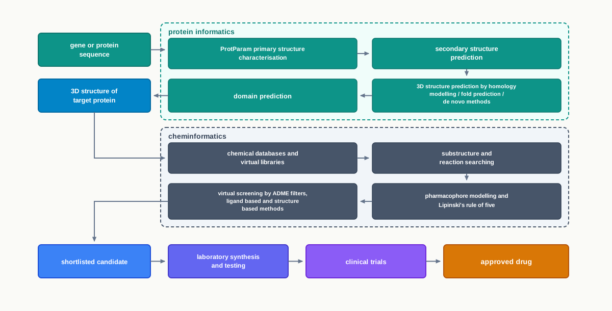
The chapter as a whole moves from a raw sequence to a marketed medicine, and that overall sequence is condensed in Fig. 10.9.

Fig. 10.9

Fig. 10.9 – Protein informatics and cheminformatics pipeline.

10.4 Key Terms

  1. Protein informatics — The collection, storage and analysis of information about any protein using the techniques of information technology.

  2. Hypothetical protein — A protein whose sequence has been derived directly from a genomic sequence but for which there is no known evidence of existence.

  3. Functional site — The specific region on a folded protein, such as a pocket or groove, where a substrate or partner molecule binds.

  4. Biochemical function — The chemical reaction or activity that a protein carries out.

  5. Biological function — The role that a protein’s activity plays in the life of the organism.

  6. Tertiary structure — The complete three-dimensional folded shape of a single polypeptide chain.

  7. Heterogeneous databases — Collections of different kinds of biological information, held in different formats and at different centres, that can nevertheless be searched together.

  8. Descriptor — A measurable number or code standing for a property of a molecule, allowing molecules to be compared mathematically.

  9. Proteome — The complete set of proteins expressed by an organism.

  10. MALDI (Matrix Assisted Laser Desorption Ionisation) — A mass-spectrometry technique in which a laser is used on a matrix-embedded sample to produce short protein sequence reads.

  11. NMR (Nuclear Magnetic Resonance) — A technique that reports on the environment of atomic nuclei in a magnetic field and yields structural information about proteins in solution.

  12. MS (Mass Spectrometry) — A technique that measures very accurate molecular masses of proteins and their fragments.

  13. Multi-fractal property — A texture that repeats at different magnifications and needs several numbers to describe it, used to design protein-markers from images of heat-denatured aggregates.

  14. Network mapping — The construction of maps showing which protein influences which, used to identify possible targets for treatment of diseases.

  15. Wavelet techniques — Image-analysis methods that break an image into patterns at several scales.

  16. Homology — The degree of similarity between the sequences of two proteins.

  17. Structure optimisation — Adjustment of a rough structural model until its atoms occupy energetically sensible positions.

  18. ANN, SVM and HMM — Artificial Neural Network, Support Vector Machine and Hidden Markov Model; statistical and machine learning techniques that learn rules from known examples and apply them to unknown proteins.

  19. SBML (Systems Biology Mark-up Language) — A standard computer language for writing biological models so that they can be exchanged between laboratories.

  20. High throughput screening — The ability to run the same analysis on very large numbers of samples or compounds one after another without extra manual work.

  21. ProtParam — The tool of the ExPASy Proteomics Server that computes the physico-chemical properties of a protein from its sequence.

  22. ExPASy Proteomics Server — The proteomics resource that hosts ProtParam and related analysis tools.

  23. Isoelectric point (pI) — The pH at which the surface of a protein is covered with charge but its net charge is zero, at which the protein is stable and compact.

  24. Isoelectric focusing — A purification method in which proteins migrate through a pH gradient and each stops at the pH equal to its own pI.

  25. Aliphatic index (AI) — The relative volume of a protein occupied by aliphatic side chains (A, V, I and L), a positive factor for thermal stability of globular proteins.

  26. Instability index — An index computed from destabilising dipeptides that estimates the stability of a protein in a test tube; below 40 predicts stability, above 40 instability.

  27. Grand Average Hydropathy (GRAVY) value — The sum of the hydropathy values of all the amino acids divided by the number of residues, a low value indicating better interaction with water.

  28. Secondary structure — The local, regularly repeating folds of the protein backbone, chiefly α-helices and β-pleated sheets.

  29. APSSP, CFSSP, SOPMA and GOR — Common computational tools for protein secondary structure prediction.

  30. Homology modelling — Prediction of the structure of an unknown protein by aligning its sequence against proteins of known structure and borrowing their fold.

  31. Chou-Fasman method — A method that uses lower degrees of homology to determine local structures, used for predicting secondary structure.

  32. MODELLER and SWISS-MODEL — Commonly used tools for homology modelling.

  33. Fold prediction (threading) — A method in which the sequence of an unknown protein is forced to take the backbone conformation of a protein of known structure.

  34. LIBELLULA and Threader — Commonly used tools for fold prediction by threading.

  35. De novo protein structure prediction — An algorithmic process in which the tertiary structure is predicted from the amino acid primary sequence alone, without a template.

  36. Ab initio — Meaning “from the beginning”; describing structure prediction built from first principles, as implemented in the QUARK algorithm.

  37. PDB file — A text file with the extension .pdb that stores the three-dimensional atomic coordinates of a structure.

  38. Protein Data Bank (PDB) — The database of biomolecular structures containing data from X-ray crystallography, NMR and a few theoretical structure models.

  39. Domain — A distinct structural and/or functional unit of a protein that folds independently and carries a specific function.

  40. InterPRO and CDD — The most common tools for domain prediction, InterPRO scan of EMBL and CDD search of NCBI.

  41. Cheminformatics — The use of computational and informational techniques to understand problems of chemistry, also called chemoinformatics or chemical informatics.

  42. Computer-aided drug design (CADD) — The use of cheminformatics to look for molecules with specific biological and therapeutic properties.

  43. Virtual library — A collection of chemical compounds that exist as data rather than as substances, including hypothetical compounds along with their likely synthesis methods and predicted stability.

  44. Combinatorial techniques — Synthetic methods in which chemical building blocks are combined in every possible arrangement to generate a very large family of related molecules.

  45. CAS (Chemical Abstracts Service) — A division of the American Chemical Society that maintains the world’s largest collection of chemistry insights and serves as a universal standard for chemical names and structures.

  46. In silico — Meaning “inside a computer”; used for work done computationally, alongside in vivo and in vitro.

  47. Molecular graph — A computer representation of a chemical structure in which nodes stand for atoms and edges stand for bonds.

  48. Node and edge — In a graph, a node is a unit of chemical substance and an edge is the movement of information between nodes.

  49. Substructure retrieval — A search that returns all compounds containing a specified structural feature, such as a methyl group or benzene ring.

  50. Subgraph isomorphism — The complete embedding of a small graph into a larger one, the computational basis of substructure searching.

  51. Two-stage search — A search strategy in which most molecules are first filtered out cheaply, and the elaborate subgraph test is applied only to the small surviving set.

  52. Bitstrings — Binary strings of 0s and 1s used to implement molecule screens by recording the presence or absence of structural features.

  53. Atom mapping — Finding an exact correspondence between the atoms of the reactants and the atoms of the resulting products in a reaction search.

  54. Pharmacophore — An ensemble of the steric and electronic features necessary to ensure optimal interaction with a specific biological target and to trigger a biological response.

  55. 3D pharmacophore — A set of pharmacophore features described in terms of their spatial orientation, such as charged groups, rings and hydrophobic regions.

  56. Lipinski’s rule of five (RO5) — A set of four criteria, proposed in 1997, describing the molecular properties expected of an orally active drug, with not more than one violation permitted.

  57. log P — The octanol–water partition coefficient, a dimensionless measure of how strongly a compound prefers a lipid environment over water.

  58. ADME — Absorption, Distribution, Metabolism and Excretion; the properties describing what the body does to a drug.

  59. Ligand based methods — Virtual screening methods, including machine learning techniques and pharmacophore based search, that rely on molecules already known to be active.

  60. Structure based methods — Virtual screening methods, including protein-ligand docking, that rely on the three-dimensional structure of the target.

  61. Protein-ligand docking — Computational placement of a candidate molecule into the binding site of a target protein to score how well it fits.

  62. Virtual screening — The in silico scoring, ranking and extraction of promising structures from large libraries of real and virtual molecules using increasingly stringent filters.

  63. High Throughput Screening (HTS) — A large scale automated process in which millions of compounds are tested for a desired property.

  64. Hits — Activity observed during high-throughput screening, defined by the percent activity of new compounds compared with well defined known compounds.

  65. False positive — A compound found active in an assay that turns out to be inactive towards a certain biological target.

  66. Lead compound — A compound that is biologically and pharmacologically active with desired properties and can be processed further.

  67. Library — An inventory of compounds that fulfil the criteria for screening against specific cellular targets.

  68. New Chemical Entity — A novel molecule discovered in the laboratory that has not yet entered clinical trials.

  69. Off target activity — Molecular interactions between chemical compounds and cellular molecules that do not bind the intended target.
10.5 Points to Ponder

  1. Anfinsen’s experiment showed that the folded shape of a protein is decided entirely by its amino acid sequence. If that is true, why has predicting structure from sequence remained such a difficult problem for so long?

  2. Structure prediction can be carried out even when only a gene sequence is available. Does a predicted structure carry the same scientific weight as one determined by X-ray crystallography? What would convince you that a predicted model is trustworthy?

  3. The instability index uses a cut-off of 40, and Lipinski’s rule of five uses cut-offs of 5, 10, 500 Daltons and log P 5. What is gained by fixing sharp numerical boundaries on properties that in reality vary continuously, and what is lost?

  4. Lipinski’s rule permits one violation, and does not apply to natural products or to drugs given by injection. What does a rule with this many exceptions actually tell a researcher, and how should such a rule be used?

  5. A hypothetical protein is identified only inside a computer. At what point would you say that this protein has been “discovered” — when its gene is sequenced, when its structure is predicted, or when it is finally isolated in a laboratory?

  6. Storing a molecule as an image is nearly useless for research, while storing it as a graph of nodes and edges opens up every kind of search. What does this suggest about the relationship between how information is represented and what can be done with it?

  7. Both the Viagra and saccharin stories describe discoveries made by accident. If cheminformatics succeeds in filtering out everything that does not match a predicted requirement, could it also filter out the next accidental discovery? How might a research programme protect itself against this?

  8. Virtual screening reduces the number of compounds that must be tested on animals and humans. Yet regulators still insist on Phase I, II and III trials. Is this insistence a failure of trust in computation, or a necessary safeguard? Argue both sides before deciding.

  9. The Protein Data Bank grew because scientists agreed to deposit their hard-won structures where anyone could use them. What would the field of protein informatics look like today if structures had instead been kept private by the laboratories that solved them?

  10. Domains recur in unrelated proteins, carrying the same function each time. What does this repetition suggest about how proteins may have evolved, and how does it help a scientist guess the function of a newly sequenced protein?

  11. A compound that is active in an assay may turn out to be a false positive, and a compound may bind molecules other than its target (off target activity). Why can no amount of computational filtering completely remove these two problems?

  12. The drug pipeline takes roughly thirteen to nineteen years and ends with a single approved compound out of thousands. Where in this pipeline would you invest additional effort to reduce the failure rate, and why?

10.6 NCERT Questions

  1. What is the role of information technology in determination of protein properties?

  2. What type of protein raw data is used for computationally extracting information about the protein?

  3. Name any two common tools for domain prediction.

  4. What is the significance of cheminformatics?

  5. Which of the following is not a rule in Lipinski’s rule of five (RO5)?

    1. No more than 10 hydrogen bond receptors
    2. Partition coefficient logP of less than 5
    3. Not more than 5 hydrogen bond donors
    4. Molecular weight above 500g/mol
  6. Which of the following properties of protein is not included in primary structure prediction?

    1. Aliphatic index
    2. Fold prediction
    3. Instability index
    4. Isoelectric point

10.7 Objective Questions

  1. Protein informatics is best described as —

    1. the purification of proteins using chromatography
    2. the collection of information about proteins using techniques of information technology
    3. the chemical synthesis of peptides in the laboratory
    4. the crystallisation of proteins for X-ray studies
  2. A protein sequence derived directly from a genomic sequence, with no known evidence of existence, is called a —

    1. recombinant protein
    2. denatured protein
    3. hypothetical protein
    4. conjugated protein
  3. MALDI, as a source of protein raw data, provides —

    1. atomic coordinates of the folded protein
    2. fragmented short sequences that are used to find the full length sequence
    3. images of heat-denatured aggregates
    4. a list of interacting partner proteins
  4. The multi-fractal property of a microscopic image of a heat-denatured protein aggregate is used for —

    1. predicting the tertiary structure
    2. designing a protein-marker
    3. calculating the isoelectric point
    4. mapping protein interaction networks
  5. Which of the following is a machine learning technique listed among the informatics tools used in protein informatics?

    1. SBML
    2. MALDI
    3. Hidden Markov Model (HMM)
    4. Isoelectric focusing
  6. The physico-chemical properties of a protein’s primary structure can be computed using —

    1. the SOPMA tool
    2. the ProtParam tool of the ExPASy Proteomics Server
    3. the CDD search of NCBI
    4. the QUARK algorithm
  7. A protein has a computed isoelectric point of 5.4. This indicates that the protein is —

    1. basic in character
    2. acidic in character
    3. neutral and uncharged at every pH
    4. unstable in a test tube
  8. A protein is predicted to be unstable in a test tube if its instability index is —

    1. exactly zero
    2. smaller than 40
    3. above 40
    4. equal to its aliphatic index
  9. The aliphatic index of a protein is defined as the relative volume occupied by the side chains of —

    1. A, V, I and L
    2. D, E, K and R
    3. S, T, C and M
    4. F, W, Y and H
  10. The GRAVY value of a protein is obtained by —

    1. multiplying the hydropathy values of all amino acids
    2. dividing the sum of hydropathy values by the number of residues
    3. subtracting the smallest hydropathy value from the largest
    4. dividing the molecular weight by the number of residues
  11. Which set consists only of secondary structure prediction tools?

    1. MODELLER, SWISS-MODEL, QUARK
    2. APSSP, CFSSP, SOPMA, GOR
    3. InterPRO, CDD, PDB
    4. LIBELLULA, Threader, ProtParam
  12. In the method called ‘threading’, the sequence of a protein with unknown structure is —

    1. aligned only against sequences of the same organism
    2. forced to take the backbone conformation of a protein with known structure
    3. folded purely from first principles with no template
    4. translated back into its gene sequence
  13. QUARK is a computer algorithm used for —

    1. homology modelling
    2. domain prediction
    3. ab initio protein structure prediction
    4. reaction searching
  14. The most common tools for domain prediction are —

    1. MODELLER of EMBL and GOR of NCBI
    2. InterPRO scan of EMBL and CDD search of NCBI
    3. ZINC of EMBL and ChEMBL of NCBI
    4. ProtParam of ExPASy and SOPMA of NCBI
  15. Computationally elucidated protein structures are stored as atomic coordinates in files with the extension —

    1. .jpg
    2. .sbml
    3. .pdb
    4. .tif
  16. Which database is described as a binding affinity database of small molecules for their protein targets?

    1. PharmaGKB
    2. BindingDB
    3. SuperDrug
    4. ChemSpider
  17. In a molecular graph, the nodes and edges respectively represent —

    1. bonds and atoms
    2. units of chemical substances and the connections between them
    3. reactants and products
    4. hydrogen bond donors and acceptors
  18. The complete embedding of a small graph into a larger one is known as —

    1. atom mapping
    2. subgraph isomorphism
    3. docking
    4. threading
  19. Binary strings of 0s and 1s used to implement molecule screens are called —

    1. descriptors
    2. bitstrings
    3. pharmacophore points
    4. hits
  20. Finding an exact correspondence between reactant atoms and the atoms of the resulting products is called —

    1. substructure retrieval
    2. atom mapping
    3. virtual screening
    4. network mapping
  21. According to IUPAC, a pharmacophore is —

    1. a molecule that binds to a receptor
    2. an ensemble of steric and electronic features necessary for optimal interaction with a specific biological target
    3. a group of molecules with identical structures
    4. the active site of a receptor protein
  22. Lipinski’s rule of five was proposed in —

    1. 1879
    2. 1971
    3. 1997
    4. 2007
  23. According to Lipinski’s rule of five, an orally active drug should have a molecular weight —

    1. below 500 Daltons
    2. above 500 Daltons
    3. exactly 500 Daltons
    4. below 50 Daltons
  24. Based on the RO5, a predicted chemical compound is assigned a value between 0–4. A compound is considered unsuitable for further analysis if its value is —

    1. equal to 4
    2. equal to 3
    3. less than 3
    4. more than 3
  25. Protein-ligand docking is an example of —

    1. a general ADME filter
    2. a ligand based method
    3. a structure based method
    4. a secondary structure prediction method
  26. In the drug development pipeline, the Development stage is associated with —

    1. 5–6 years and thousands of compounds
    2. 7–8 years and 1–5 compounds
    3. 1–5 years and 1 compound
    4. 13–19 years and a single idea
  27. A compound found active in an assay that later turns out to be inactive towards a certain biological target is termed a —

    1. hit
    2. lead compound
    3. false positive
    4. new chemical entity
  28. Assertion (A): Protein structure prediction is possible even when the protein sequence itself is not available. Reason (R): A known gene sequence can be translated computationally into the corresponding amino acid sequence, from which prediction proceeds.

  29. Assertion (A): At its isoelectric point a protein is stable and compact. Reason (R): At the isoelectric point the surface of the protein carries no charged groups at all.

  30. Assertion (A): A very high aliphatic index suggests that a protein may remain stable over a wide temperature range. Reason (R): The aliphatic index measures the relative volume of the protein occupied by aliphatic side chains, which contribute to the thermal stability of globular proteins.

  31. Assertion (A): Secondary structure prediction is useful even when the final aim is a three-dimensional model. Reason (R): Prediction of secondary structure is regarded as a step towards protein 3-dimensional structure prediction.

  32. Assertion (A): Fold prediction methods are more compute-intensive than homology modelling methods. Reason (R): Fold prediction gives more confidence in the physical viability of the results.

  33. Assertion (A): Substructure searching is usually carried out as a two-stage process. Reason (R): The full subgraph isomorphism test is computationally expensive, so a rapid screen is used first to eliminate most molecules.

  34. Assertion (A): A pharmacophore cannot be isolated or synthesised in a laboratory. Reason (R): A pharmacophore is a conceptual framework describing molecular features, not a physical molecule or group of molecules.

  35. Assertion (A): Lipinski’s rule of five may not apply to a drug administered intravenously. Reason (R): The rule was framed to identify compounds that can be successful as orally active drugs.

  36. Assertion (A): Storing chemical structures as image files is of little use in research demanding ‘deep browsing’. Reason (R): An image file does not record which atom is joined to which, so bond angles and rotational flexibility cannot be examined from it.

  37. Assertion (A): Virtual screening applies its cheapest and broadest filters first. Reason (R): As one moves from the first step of virtual screening to the last, the criteria get increasingly stringent.

10.8 Check Your Concepts

  1. Why is protein informatics described as a science that depends on information technology rather than on laboratory equipment? Explain with reference to the kind of raw data it uses.

  2. Distinguish between the biochemical function and the biological function of a protein, giving one example of each.

  3. A newly sequenced bacterial genome yields 400 protein sequences, of which 130 have no experimental evidence of existence. What are such proteins called, and describe the sequence of computational steps you would follow to suggest a possible function for one of them.

  4. Explain why the availability of large public databases is a precondition for machine learning methods such as ANN, SVM and HMM to work in protein informatics.

  5. Match the following protein data types with the information they yield.

Column A Column B
a. Microscopic image of heat-denatured aggregate i. Study of mutations and interactions
b. Protein in solution ii. Designing protein-markers using multi-fractal property
c. Protein crystal structure iii. Identification of possible drug targets
d. Fragmented sequences from MALDI iv. Physico-chemical properties and kinetics
e. Network mapping data v. Reconstruction of the full length sequence
  1. Arrange the following in the correct order as they occur in a structure prediction workflow: fold prediction, database searching, protein sequence, 3-D protein model, multiple sequence alignment, secondary structure prediction.

  2. Look at Fig. 10.2. What decision is taken at the step marked “homologue in PDB?”, and what are the two different paths that follow from it?

  3. Why does a researcher compute the isoelectric point of a protein before attempting to purify it? What would go wrong if a buffer of the wrong pH were chosen for isoelectric focusing?

  4. At its isoelectric point, the surface of a protein is described as “covered with charge” and yet the net charge is zero. Explain how both statements can be true at the same time.

  5. Two recombinant proteins are expressed for a laboratory experiment. Protein X has an instability index of 28 and Protein Y has an instability index of 52. Which one would you expect to survive better in a test tube, and why?

  6. A thermophilic bacterium lives in a hot spring. Would you expect its enzymes to have a high or a low aliphatic index? Justify your answer in terms of the side chains involved.

  7. Explain why a low GRAVY value suggests that a protein interacts well with water, while a high value would raise the possibility of a membrane-associated protein.

  8. Why is secondary structure prediction described as “a step towards” three-dimensional structure prediction rather than an end in itself?

  9. Compare homology modelling, fold prediction and de novo prediction on the basis of (i) the template required, (ii) computing demand, and (iii) the situation in which each is the only usable option.

  10. A protein of unknown structure shows very low sequence similarity to every entry in the PDB. Which prediction method would you avoid, which would you try next, and why?

  11. An advantage of homology modelling is stated to be its “lack of dependence on the knowledge of physical determinants”. Explain what this means and why it makes the method faster.

  12. Draw a simple diagram of a polypeptide chain folded into two domains joined by a linker, and label the domains, the linker and one functional site. Why is domain prediction so valuable for a newly identified hypothetical protein?

  13. A student saves a chemical structure as a .jpg image and claims it can be used for substructure searching. Identify the error in this approach and state how the structure should actually be stored.

  14. Explain, using the idea of subgraph isomorphism, how a database returns every compound containing a benzene ring when that ring is drawn as a query.

  15. A junior researcher proposes running the full subgraph isomorphism test directly on a database of 200 million compounds, without any screening step. Explain what is wrong with this protocol and rewrite it correctly.

  16. The same node-and-edge representation is used both for a single molecule and for a metabolic pathway such as glycolysis. Explain what the nodes and edges stand for in each case.

  17. Why does a chemist planning a synthesis need information on solvents, pH, temperature and pressure, and not merely the identity of the product? Frame one refined reaction query that combines two such conditions.

  18. Two drugs with completely different chemical structures act on the same receptor. Explain how the concept of a pharmacophore accounts for this observation.

  19. “A pharmacophore is not a physical molecule.” Defend this statement, and explain why a pharmacophore is still useful in searching chemical databases.

  20. Explain the physical reason behind each of the four criteria of Lipinski’s rule of five. Why does the rule not apply to a drug given intravenously?

  21. A plant-derived compound violates two of Lipinski’s criteria. A student concludes that it cannot possibly be a useful medicine. Comment on this conclusion.

  22. Compare ligand based methods and structure based methods of virtual screening. Under what circumstances would a researcher be forced to use the ligand based approach?

  23. Why does virtual screening apply broad ADME-based filters before protein-ligand docking, and not the other way round? What would be the practical consequence of reversing the order?

  24. Distinguish between a hit, a lead compound and a new chemical entity, and place each at its correct position in the drug discovery pipeline.

  25. Explain the difference between a false positive and off target activity. Why is it important for a screening programme to detect both as early as possible?

  26. Study Fig. 10.7. Roughly how many years pass between the initial idea and the drug reaching patient care, and at which stage does the number of surviving compounds fall most sharply? What does this tell you about the value of early computational filtering?

  27. Protein informatics and cheminformatics are treated as two halves of a single process in drug discovery. Explain how the output of the first becomes the input of the second.

10.9 Case-Based Questions

  1. A research group sequences the genome of a soil bacterium and translates its coding regions on a computer. Out of the proteins obtained, 96 have no experimental evidence of existence. One of them is 240 amino acids long. The group has no purified sample, no crystal and no antibody against this protein, but wishes to suggest a function for it within a month.

    1. What term is used for the 96 proteins described here?
    2. State the two basic facilities the group must have in place before any protein informatics analysis can begin.
    3. Outline, in order, the computational steps the group would follow to move from the translated sequence to a suggested biological function.
    4. Why is this approach described as offering advantages of time frame, low cost and high throughput screening?
  2. A student submits the sequence of a 310-residue protein to the ProtParam tool of the ExPASy Proteomics Server and obtains the following output.

Property Computed value
Isoelectric point (pI) 8.6
Aliphatic index 96.4
Instability index 47.2
GRAVY value \(-0.412\)
a. Is this protein acidic or basic in character? Give the reason.
b. Comment on the likely stability of the protein in a test tube, quoting the relevant cut-off value.
c. What does the GRAVY value suggest about the protein's interaction with water?
d. The student wants to purify this protein by isoelectric focusing. Which of the computed values will be most useful, and how will it be used?
  1. A laboratory needs a three-dimensional model of an enzyme from a newly described fungus. The sequence is submitted to a database search. No protein in the PDB shows appreciable homology to it. Secondary structure prediction is then carried out, followed by fold prediction, but no acceptable fold is obtained either.

    1. Which prediction method has been ruled out by the first result, and why?
    2. Name two tools that could have been used had a good homologue been found.
    3. Which method must the laboratory now fall back on, and name one algorithm used for it.
    4. Once the model is built, in what file format and in which database would the coordinates be stored?
  2. A pharmaceutical company has identified a receptor protein as the target for a new medicine. Its chemical database holds around 180 million real compounds and a virtual library of several billion hypothetical compounds. The medicinal chemists know that all previously active molecules at this receptor carry a benzene ring linked to a positively charged group.

    1. Which type of search would retrieve every compound in the database carrying that benzene ring, and on which computational idea does it rest?
    2. Explain why the search is carried out in two stages, and state what bitstrings contribute to the first stage.
    3. The chemists then build a model from the features shared by the known active molecules. What is this model called, and what kind of features does it contain?
    4. Why is the company willing to include compounds from the virtual library, which have never been synthesised?
  3. Four candidate molecules are examined before laboratory synthesis. Their properties are listed below.

Compound Molecular weight (Da) H-bond donors H-bond acceptors log P
P 412 3 7 4.1
Q 528 6 12 5.6
R 465 5 11 3.2
S 289 2 5 1.8
a. Apply Lipinski's rule of five to each compound and state the number of violations in each case.
b. Which compounds may be taken forward as potential orally active drugs, and which should be set aside?
c. Compound Q is a semi-synthetic derivative of a natural product. Does this change your assessment? Explain.
d. All four compounds are to be given by intravenous injection instead. Explain how this alters the usefulness of the rule.
  1. A start-up announces that its computational platform can screen billions of compounds, predict their toxicity, and identify a safe medicine without any animal or human testing. It requests permission to market a compound directly on the strength of its in silico results. The regulatory authority refuses, and insists on the standard pipeline.

    1. Name the three stages of the drug development pipeline and the approximate time each takes.
    2. Give two scientific reasons, drawn from the chapter, why a computational prediction of safety cannot be treated as final.
    3. State one genuine benefit that the start-up’s approach offers to patients and to laboratory animals.
    4. Write a short, balanced argument on how far a regulator should allow computational evidence to replace experimental evidence.
  2. In the early 1990s, a compound coded UK92480 was tested for relaxing blood vessels and treating heart complications. It performed poorly for that purpose, but an unexpected effect on another system led to its development as a well known medicine. Around a century earlier, a chemist working on coal tar derivatives noticed an intense sweetness on his unwashed hands and traced it to an impure solution in one of his beakers, which turned out to be saccharin.

    1. What do both these episodes have in common regarding the way the discovery was made?
    2. Virtual screening works by eliminating compounds that fail to match a set of predefined criteria. Explain how such a system might have missed both of these discoveries.
    3. Suggest one way in which a modern research programme can retain the benefits of computational filtering while still leaving room for unexpected findings.

10.10 Practice With Data

  1. A peptide is 40 residues long. The hydropathy values of its residues add up to \(+34.8\). Calculate its GRAVY value using \[\mathrm{GRAVY} = \frac{\displaystyle\sum_{i=1}^{n} h_i}{n}\] and state whether the peptide is more likely to interact well with water or to associate with a lipid environment. Give the reason for your answer.

  2. Two proteins are analysed with ProtParam. Protein A has 180 residues and a total hydropathy of \(-90.0\); Protein B has 250 residues and a total hydropathy of \(-45.0\). Calculate the GRAVY value of each and state which of the two is more likely to be soluble in an aqueous buffer.

  3. The table below gives ProtParam output for four recombinant proteins.

Protein pI Aliphatic index Instability index GRAVY
W 4.8 71.2 33.5 \(-0.520\)
X 9.2 105.6 51.8 \(+0.240\)
Y 6.4 88.0 39.6 \(-0.180\)
Z 7.9 62.5 44.1 \(-0.610\)
a. Classify each protein as acidic or basic.
b. List the proteins predicted to be stable in a test tube, and those predicted to be unstable.
c. Which protein is most likely to remain stable over the widest temperature range?
d. Which protein shows the greatest likelihood of good interaction with water?
  1. A protein has a computed pI of 6.2 and is to be purified by isoelectric focusing over a pH gradient running from 3 to 10. At approximately what point in the gradient will this protein stop moving? Explain your reasoning in terms of net charge.

  2. The following data describe five candidate compounds screened against a receptor.

Compound Molecular weight (Da) H-bond donors H-bond acceptors log P
C1 348 2 6 2.4
C2 512 4 9 4.6
C3 476 7 12 5.8
C4 395 5 10 4.9
C5 620 8 14 6.7
a. For each compound, count the number of Lipinski criteria violated.
b. Which compounds satisfy the rule as stated (not more than one violation)?
c. Rank the five compounds from most to least promising as orally active drug candidates, and justify the position of the compound you rank last.
  1. A compound is shaken between octanol and water. At equilibrium its concentration in the octanol layer is \(2.5 \times 10^{-3}\) mol L\(^{-1}\) and in the water layer is \(2.5 \times 10^{-6}\) mol L\(^{-1}\). Using \[\log P = \log_{10}\left(\frac{C_{\text{octanol}}}{C_{\text{water}}}\right)\] calculate the log P value, and state whether the compound satisfies the log P criterion of Lipinski’s rule of five.

  2. A substructure search is run on a database of 240 million compounds. The stage-one bitstring screen retains 0.05 per cent of the entries for the stage-two subgraph isomorphism test.

    1. How many compounds enter stage two?
    2. If the stage-two test takes 0.4 milliseconds per compound, how much total time does stage two require? Express the answer in minutes.
    3. Estimate how long stage two alone would have taken had it been applied to the whole database, and comment on why the two-stage design is used.
  3. The CAS registry is described as holding more than 219 million organic and inorganic substances, more than 70 million protein and nucleic acid sequences, and more than 8 billion property values of substances.

    1. Calculate the average number of property values recorded per substance, using the figure for organic and inorganic substances.
    2. Express the number of protein and nucleic acid sequences as a percentage of the number of organic and inorganic substances.
    3. What do these figures suggest about why manual searching of chemical literature is no longer practical?
  4. Study the drug development pipeline in Fig. 10.7. The Discovery stage takes 5–6 years and begins with thousands of compounds; Development takes 7–8 years and carries 1–5 compounds; Delivery takes 1–5 years and ends with 1 compound.

    1. Calculate the minimum and maximum total time from idea to patient care.
    2. If a company begins Discovery with 5000 compounds and 3 compounds enter Development, calculate the percentage of compounds eliminated during Discovery.
    3. If only 1 of those 3 compounds is finally approved, calculate the overall success rate from the starting library, expressed as a percentage.
  5. A virtual screening run begins with 2.4 billion molecules. The ADME filter removes 92 per cent of them. Ligand based pharmacophore searching removes a further 96 per cent of those remaining. Protein-ligand docking finally retains the top 0.5 per cent of the survivors.

    1. Calculate the number of molecules remaining after each of the three filters.
    2. How many molecules are finally passed on for synthesis and biological testing?
    3. Explain, using your calculated figures, why the criteria are described as becoming increasingly stringent from the first step to the last.
  6. Docking scores (more negative values indicating stronger predicted binding) are obtained for six molecules: \(-4.2\), \(-9.8\), \(-6.5\), \(-11.3\), \(-7.1\) and \(-5.0\) kcal mol\(^{-1}\).

    1. Rank the molecules from strongest to weakest predicted binding.
    2. If only the top one-third are to be synthesised, which molecules are selected?
    3. A molecule with an excellent docking score is later found to be inactive in the assay. Which term from the chapter describes this outcome, and give one possible reason for it.