Chapter 11: Programming and Systems Biology
In the early 1950s, two physiologists at Cambridge, Alan Lloyd Hodgkin and Andrew Fielding Huxley, set out to answer a question that sounds simple: what exactly is a nerve impulse? They worked on the giant axon of the squid — a nerve fibre thick enough to push fine electrodes into. Their recordings told them how sodium and potassium ions crossed the membrane. But measurement alone could not explain how those tiny ion movements built up into a travelling electrical wave that races down the whole length of a nerve.
So they did something unusual for biologists of that time. They wrote the behaviour of the membrane as a set of mathematical equations, and then solved those equations step by step on a hand-operated mechanical calculator. It was slow, grinding arithmetic that took weeks. When the numbers were finally plotted, they produced the shape of a nerve impulse that nobody had ever derived from theory — and it matched the real recording remarkably closely. Their model was published in 1952, and the work later earned them a Nobel Prize.
That calculation was biology’s first serious taste of what computation could do: not merely describe life, but predict it. Today a laptop redoes it in a fraction of a second — and biologists now use code to model whole cells.

Fig. 11.0 – Manual computation versus modern systems modeling.
Keep these questions in mind as you read — this chapter will answer every one of them.
11.1 Programming in Biology
Not very long ago, a biologist worked mostly with numbers that could be counted by hand — the number of colonies on a plate, the readings from a spectrophotometer, the bands on a single gel. Calculations were done manually, and a large experiment meant a few hundred data points. That era is now behind us.
Today biology sits in a phase of high-throughput data generation, automated analysis and prediction. A single sequencing run can read billions of bases. A single microarray or proteomics experiment can report on thousands of genes or proteins at once. Machines generate the data; software must make sense of it.
Technological advancement has been a genuine boon here. Volumes of data that were unthinkable a few decades ago are now produced routinely in ordinary laboratories, and a task that looked gigantic a decade back appears trivial now.
The Other Side of Big Data
But the arrival of massive data has also thrown massive challenges. These challenges fall into five connected areas, and it is worth seeing why each one is a real problem.
Storage — genome-scale files are far too large for an ordinary hard disk, so data must be kept on servers or in the cloud, in compressed and well-organised form.
Visualisation — a table of ten million numbers tells a human nothing. The data must be turned into plots, heat maps or network pictures before a scientist can see a pattern in them.
Transfer — collaborators sitting in different countries must be able to move these enormous files reliably, without corruption.
Analysis — the raw output of a machine is not an answer. It has to be cleaned, filtered, corrected for errors and then tested statistically.
Interpretation — finally, the analysed result must be read back into biology: which gene, which pathway, which disease.
The overall path from a machine’s raw output to a biological conclusion is worth fixing in your mind before we look at individual languages; it is summarised in Fig. 11.1.
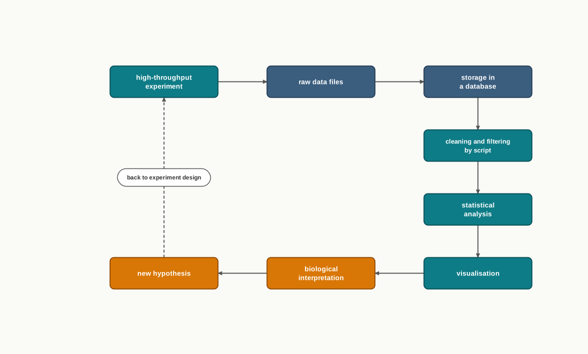
Fig. 11.1 – Path of high-throughput biological data.
Why Programming Now Matters to a Biologist
The emergence of artificial intelligence (AI) and machine learning (ML) techniques has changed research practice in almost every field, and biology is no exception. These methods learn patterns from very large training data sets and then make predictions — for example, predicting the structure a protein will fold into, or which patients are likely to respond to a drug.
Because of this, it is increasingly evident that young biotechnology students working at the cutting edge of science may, in future, require basic programming knowledge along with comfort in chemistry and statistical methods. The biologist of the coming decade is expected to design the experiment and also to handle the data it produces.
The purpose of this chapter is not to give an exhaustive description of programming languages. It is to offer a gentle introduction to some of the most popular high level languages that are relevant to biologists.
Platforms and the Place of Linux
Bioinformatics software is being developed for all the available operating system (OS) platforms, but the majority of successful applications have been developed on the Linux platform. There are practical reasons for this: Linux is free, it is stable when a program has to run for many hours without stopping, it handles very large files comfortably, and its command line makes it easy to chain small tools together and automate repetitive jobs. Most high-performance computing clusters and web servers also run Linux.
From the beginning of bioinformatics, PERL has always been at the core of sequence-based large data handling. Sequence work is essentially text work — searching for a motif, splitting a file, reformatting millions of records — and PERL was built to be very strong at exactly this kind of pattern matching in text.
These platforms are now being enriched with more advanced performing languages. Normally, Python and R provide strong facilities of statistical packages for solving biological problems. Python modules are being continuously enriched with visualisation and analysis modules for handling large data sets, whether the work is done on a standalone computer, on a web server, or through cloud computing. In cloud computing the analysis actually runs on a remote bank of powerful machines, which is what makes genome-scale work possible from an ordinary laptop. Beyond these, MATLAB also provides a very good platform for bioinformatics data analysis.
Some of the most advanced languages active in the area of bioinformatics are described below.
Python
Python is a high level, general purpose programming language created by Guido van Rossum (1991). It is an object oriented, interactive programming language that can run on unix, mac and windows — so the same script written by a student in one laboratory will run on a collaborator’s machine elsewhere.
“Object oriented” means the language lets you bundle data and the operations on that data together into a single unit called an object. For a biologist this is convenient: a DNA sequence can be treated as an object that already knows how to give its length, its complement or its GC content.
Python is very popular within the bioinformatics community largely because of three things:
the clear meaning of the terms used and the structure of its statements, which makes Python code unusually easy to read — an important point when several people share and check the same analysis;
its expressivity and alignment to object-oriented programming, so a complex idea can be written in a few lines; and
the availability of libraries and third-party toolkits. A library is a ready-made collection of code that someone else has already written and tested, so a biologist need not build a sequence reader or a plotting routine from scratch.
Python has been used successfully for sequence and structure analyses, phylogenetics and so on.
R
The name R has been derived from its inventors, Robert Gentleman and Robert Ihaka, who developed this language. R has gained wide acceptance as a rapid and reliable functional programming language that is ideal for high volume analysis, visualisation and simulation of biological data.
The software is free and open source, which means anyone may use it and also read and modify the code behind it — an important advantage for research, where a method must be open to checking by others. The R language has been used for the analysis of genome sequences and of biomolecular pathways.
Both Python and R appear constantly in biotechnology, and students often confuse their strengths, so it helps to place them side by side.
Languages Built for Designing Living Systems
The languages discussed so far were made to analyse data that an experiment has already produced. Moving from data analysis to designing the systems themselves, new programming languages have emerged — languages in which a scientist can describe a biological system that is to be built, not merely one that has been measured.
Among them are GEC (Genetic Engineering of living Cells), a rule based language developed by Microsoft. In a rule based language the user states the rules that the parts must obey, and the software works out the arrangements that satisfy them.
The other is Kera, an object oriented, knowledge based programming language developed by Dr. Umesh P. of University of Kerala. Kera captures information on the genome, proteins and the cell, using a user edited biological library called Samhita. Because the library is user edited, the knowledge in it grows as the research community adds to it.
The full range of what a biologist may use is easier to hold in mind as a map, as shown in Fig. 11.2a.
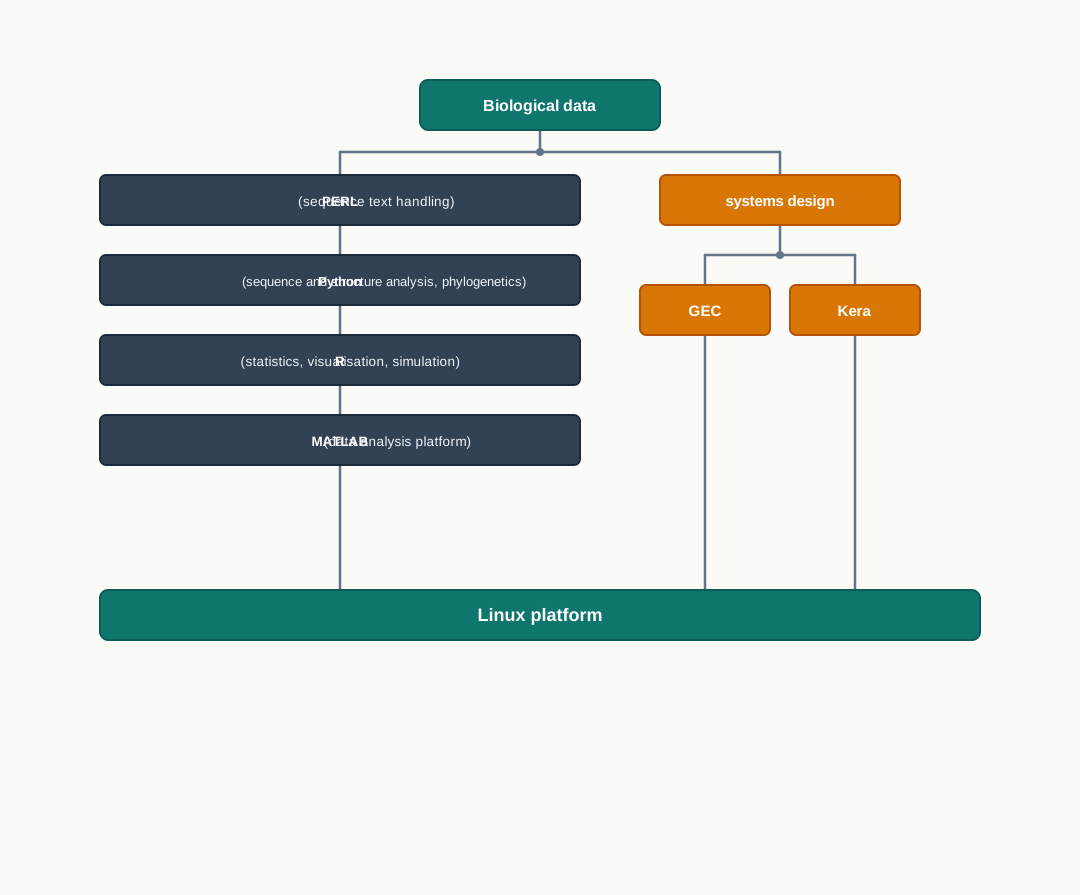
Fig. 11.2a – Programming resources for biologists.
In board and competitive examinations this section is usually tested in short, factual ways: naming the inventors of a language, matching a language with what it is used for, or picking the incorrect statement about programming in biology from four options. Learn the names, the dates and the specific use of each language carefully — that pairing of language with purpose is what such questions check.
11.2 Systems Biology
11.2.1 Introduction
To understand the mysteries of nature, scientists have been performing experiments for a very long time. The findings of these experiments are recorded as data in the scientific literature. Starting from small bits of data and moving to very large ones, this record has been built up over decades of experimental effort.
At present, a very large volume of biological data is generated and stored in digital format in a variety of storehouses called databases. A database is not simply a heap of files; it is an organised store in which every entry is labelled, indexed and searchable, so that a computer can retrieve exactly what is asked for out of millions of records.
These digital data are the resource that makes the foundation for researchers to develop computational models — models that can perform tasks similar to those of our complex biological systems, that is, the behaviour we observe in real in-vitro or in-vivo experiments, or in real life. Here in-vitro means an experiment done outside the body in glassware or culture, and in-vivo means one done inside a living organism.
Building a System Model
The implementation of such ideas is carried out with mathematical and computational models that mimic complex biological systems. These models are called system models.
Therefore, you can visualise systems biology as the representation of system models. Instead of studying one component in isolation, the scientist writes down how all the chosen components influence one another, and then lets the computer work out how the whole set behaves over time.
Nowadays systems biology has become an area of intensive research with potent applications. It is an interdisciplinary field of study that focuses on complex biological interactions within biological systems, as depicted in Fig. 11.3.
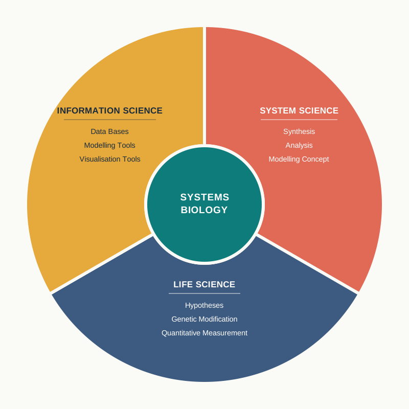
Fig. 11.3 – Systems biology as an interdisciplinary field.
Notice what Fig. 11.3 is really telling you. Systems biology does not belong to any one discipline. It needs life science to supply the hypotheses, the genetically modified material and the quantitative measurements; information science to supply the databases, modelling tools and visualisation tools; and system science to supply the concepts of synthesis, analysis and modelling. Remove any one of the three sectors and the field cannot function.
Why the Field Grew So Fast
The concept of systems biology has been adopted in a variety of biological contexts, particularly from the last two decades onwards. The Human Genome Project is one of the most glorious seedings of the thought of systems biology, and it led to the new avenues of today’s form of the field.
The reason is easy to see. Once the entire sequence of an organism was available, biologists no longer had a shortage of parts; they had a shortage of understanding about how the parts work together. That shift — from finding components to explaining their collective behaviour — is exactly the ground on which systems biology stands.
Presently, systems biology models can provide a theoretical description for the discovery of emergent functional properties of cells, tissues and organisms — properties that earlier could be found only through experiments. An emergent property is one that belongs to the whole system but to none of its parts on its own: a single heart cell cannot beat rhythmically as an organ does, and a single enzyme cannot show the steady output that a whole metabolic pathway does.
The most efficient system models are those of metabolic or signaling networks. Along with the fundamental understanding of the mechanism of action of biological systems, systems biology is intensely being utilised for potent applications — for example in the areas of health and disease, running all the way from biological networks to modern therapeutics.
11.2.2 Historical Perspective
Before the emergence of systems biology, research in the biological sciences — take, for example, the period 1900–1970 — moved around physiology, population dynamics, enzyme kinetics, control theory and cybernetics as the segmental components of research. Each of these was a separate compartment, and the idea of joining them into one quantitative picture had not yet taken hold.
The First Mathematical Models
Systems biology has been mapped as evolving from a physiological description. In 1952, Alan Lloyd Hodgkin and Andrew Fielding Huxley — both Nobel laureates — described a mathematical model for action potential propagation along the axon of a neuronal cell. You have already met this work in the chapter opener; its importance here is that it was the first time a biological process was written as equations and then successfully predicted from them.
A more evolved implementation of the theory emerged in 1960, when the first computer model of the heart pacemaker was developed by Denis Noble [PMID 13729365]. The shift is significant: the equations were now handed to a computer rather than solved by hand, and an entire tissue-level behaviour — the rhythmic beat — was reproduced in silico.
The Field Gets Its Name
Systems biology was formally launched by the systems theorist Mihajlo Mesarovic in 1966 at the Case Institute of Technology in Cleveland, Ohio, in a symposium titled “Systems Theory and Biology”. Two years later, in 1968, the first theory about systems biology was published by Ludwig von Bertalanffy, who is considered the precursor of this discipline.
The duration between the 1960s and the 1970s was the decade of development of multiple aspects of complex molecular systems, such as metabolic control analysis and biochemical systems theory. These gave biologists a formal way to ask how control over a pathway is distributed among its enzymes, rather than assuming that one “rate-limiting” enzyme decides everything.
For a time, molecular biologists were sceptical that systems theory had anything to offer their subject. This skepticism was broken by the development of theoretical biology, which includes the quantitative modelling of biological processes — once models began making testable predictions, the objection lost its force.
Since the 1990s, functional genomics has been generating large quantities of high-quality biological data, which are helping in the development of more realistic models. A model is only as good as the measurements behind it, so this flood of dependable data was what finally allowed serious modelling.
Towards a Whole Cell
In continuation of these developments, the National Science Foundation (NSF) put forward a challenge to mathematically model the whole cell. In this direction, in 2003, the Massachusetts Institute of Technology (MIT) started the search for a solution to this challenge in association with CytoSolve.
The Physiome Project
Presently, a big systems biology project, namely ‘Physiome’, is available (http://physiomeproject.org/). This project aims at developing a multi-scale modelling framework for understanding physiological function, one that allows models to be combined and linked in a hierarchical fashion.
Consider the example of the heart, illustrated in Fig. 11.4a. Electromechanical models of the heart need to be combined with models of ion channels, myofilament mechanics and signal transduction pathways at the subcellular level, and then these processes must be linked to models of tissue mechanics, wavefront propagation and coronary blood flow — each of which may well have been developed by a different group of researchers.
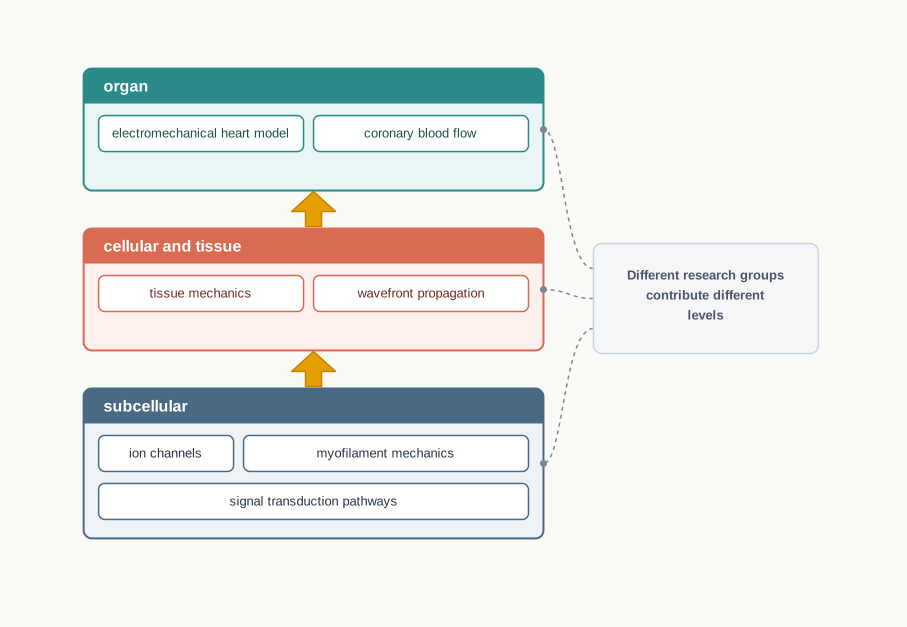
Fig. 11.4a – Multi-scale hierarchy of the Physiome approach.
This is the real difficulty of the Physiome idea. The separate models are written by different laboratories, in different software, at different scales of size and time. Making them talk to one another requires agreed standards — which is exactly the problem taken up in Section 11.2.4.
11.2.3 Theme behind the Systems Biology
To cover the diverse disciplines of biology, systems biology has been observed from different aspects. The reductionist approach worked on identification of the components and interactions of a system. It was enormously successful — it gave us genes, enzymes and receptors — but no convincing method could be evolved through it to describe the pluralism of a system.
Pluralism here means the many-sidedness of a living system: the fact that a cell is doing dozens of things at once, through components that influence one another simultaneously rather than one after the other.
Pluralism can be better observed through quantitative measures of multiple components simultaneously, and this can only be possible by mathematical models containing rigorous data integration. In this way, it can be said that systems biology is the observation of a system by integrating different components together (Fig. 11.3).
Covering all the individual components together, the core of the theme of systems biology is: ‘Object network mapping and its integration with interdependent dynamic event — kinetics with partial differential equations’.
That sentence is dense, so unpack it in three parts. Object network mapping means drawing every component as an object and every influence between objects as a link, producing a network. Integration with interdependent dynamic events means recognising that these links are not fixed pictures — each event changes with time and depends on the others. Kinetics with partial differential equations means the changes are written as rates, in equations that follow a quantity as it changes both with time and across space within the system.
11.2.4 Protocol for Systems Biology Experiments
To perform a standard systems biology experiment, discrete steps are followed, as shown in Fig. 11.5.
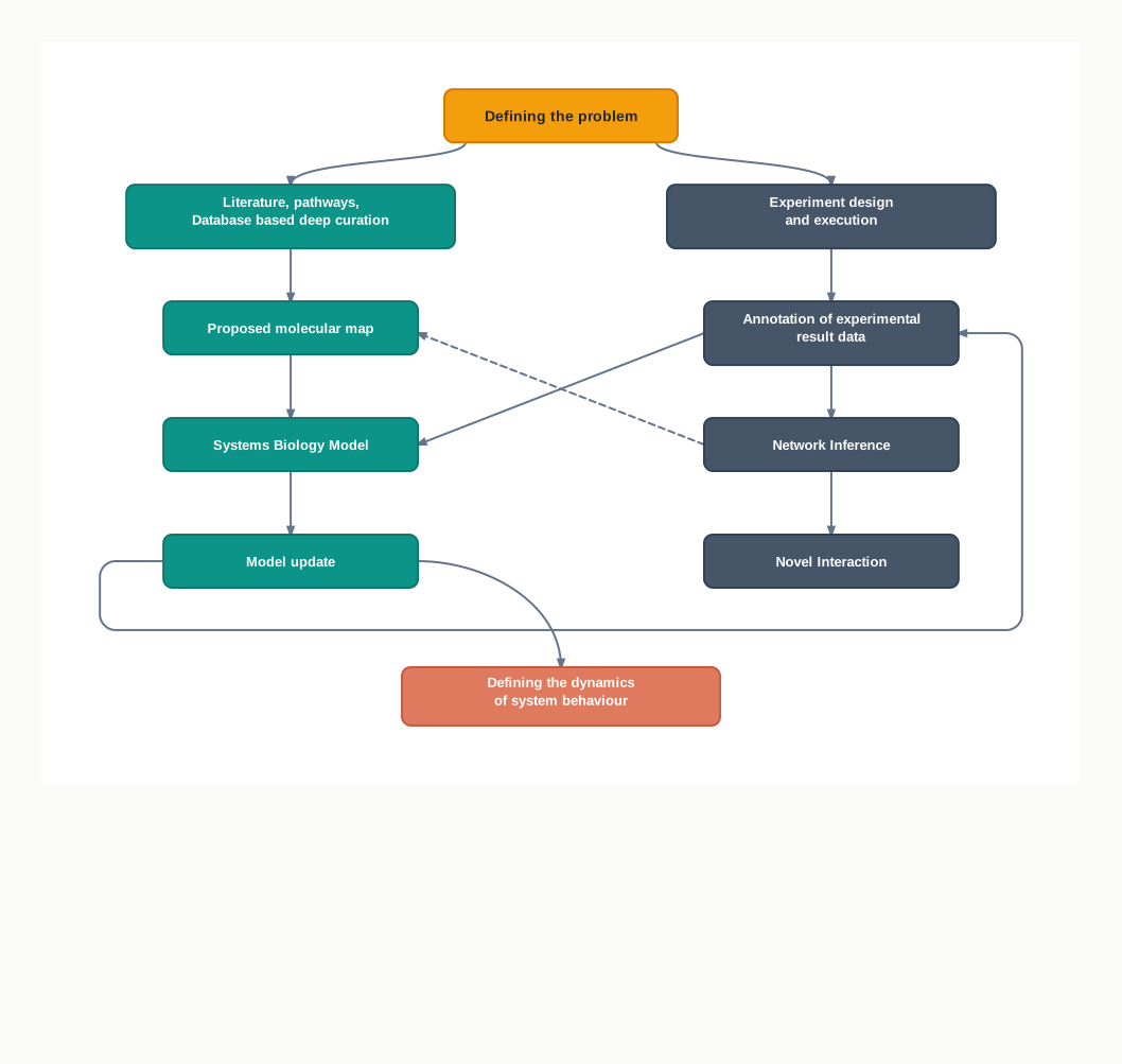
Fig. 11.5 – Workflow of a systems biology experiment.
The Steps of the Protocol
The whole protocol basically involves the definition of the problem, the designing of the experiment, the execution of the experiments to generate data, the collection of the resultant data and their arrangement in appropriate file formats, followed by the development of a network interface.
This is followed by the transfer of this network interface, which should be precise as well as mechanism based, so that the model can be developed accordingly. “Mechanism based” is an important condition: the network must record how one component acts on another, not merely that the two are correlated, otherwise the model cannot predict what happens under new conditions.
This is further followed by the analysis of discrepancies between the model-based simulation results and the experimental data, and the hypothesis is then modelled with reference to the discrepancies observed. Finally, the simulation is repeated and tested again and again, and new hypotheses are incorporated into the model.
The ordered sequence is worth committing to memory, and is set out in Fig. 11.6.
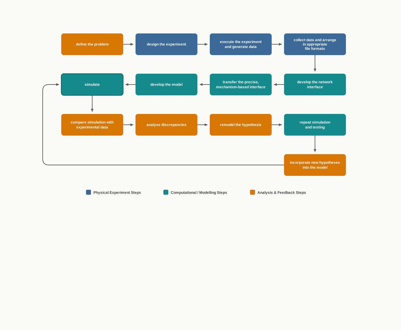
Fig. 11.6 – Protocol for a systems biology experiment.
Notice that the last arrow returns to an earlier step. A systems biology experiment is not a straight line but a cycle: each disagreement between model and data becomes the starting point of the next round. This is why the workflow in Fig. 11.5 contains loops rather than a single downward chain.
Thus, the workflow of computation for systems biology (as depicted in Fig. 11.5) requires data-management, optimisation of network development parameters, performance analysis and evaluation.
Standards for Data Management
Standards for data management have been defined for the collection of structured data for systems biology. Accordingly, three basic aspects are considered for data management, which are explained below.
(i) Minimum information
Minimum information represents a set of essential supporting information needed from different experiments such as microarray, proteomic, biological and biomedical investigations. Incorporation of metadata about these collected data is an important point to care for.
Metadata are “data about the data” — the conditions of the experiment, the organism used, the instrument, the date, the settings. Without them, a reading of “4.7” means nothing to anyone else, and the data cannot be combined with anybody else’s results.
(ii) File formats
The collected data for minimum information are stored in specific file formats. These formats are generally Extensible Markup Language (XML) based, which gives them the facility to be automatically processed by computers. In an XML-based format every value carries a tag stating what it is, so a program can pick out the right field on its own without a human having to explain the layout of the file.
(iii) Ontologies
Ontologies define a semantic annotation of data, which represents the hierarchical relationship between different terms. A few important examples are Gene Ontology (GO) and Systems Biology Ontology (SBO).
An ontology solves a very practical problem. Two laboratories may describe the same activity in different words; unless both are tied to the same term in a shared hierarchy, a computer will treat them as unrelated. Because the terms are arranged hierarchically, a search for a broad category also finds all the specific entries that sit beneath it.
Systems and Workflows in Use
Current data-management systems include spreadsheets, web-based electronic lab notebooks (ELN) and laboratory information management systems (LIMS). These systems have been customised in such a way that they can be accessed and integrated with different analysis tools and computational workflows.
Systems like Konstanz Information Miner (KNIME), caGrid23, Taverna24, Bio-STEER25 and Galaxy26 allow the construction, execution and sharing of specialised workflows. These workflows provide a computational pipeline by enabling data exchange, data integration and inter-tool communication.
The ability to share a workflow matters as much as the ability to run it: another laboratory can take the same pipeline, feed in its own data, and be certain that every step was carried out identically. A list of data management, network inference, curation, simulation, model analysis, molecular interaction and physiological modelling tools is given in Table 11.1.
Table 11.1: A resource matrix of software, tools and data resources
| Facilities | Tools / Software |
|---|---|
| Data management | Taverna, MAGE-TAB, Bio-STEER, caGrid |
| Network inference | MATLAB, R, BANJO |
| Curation | CellDesigner, PathVisio, Jdesiner |
| Simulation | MATLAB, CellDesigner, insilico IDE, ANSYS, JSim |
| Model analysis | MATLAB, BUNKI, COBRA, NetBuilder, SimBoolNet |
| Molecular interaction | AutoDock Vina, GOLD, eHiTS |
| Physiological modelling | PhysioDesigner, CellDesigner, OpenCell, FLAME |
Read Table 11.1 by facility rather than by tool name. The left column names the job to be done at a particular stage of the workflow, and the right column names the software available for that job. Notice that a few programs, such as MATLAB and CellDesigner, appear against more than one facility — they are general platforms rather than single-purpose tools.
Equations Behind the Models
These systems modelling tools include a set of interconnected partial differential equations (PDEs), which represent spatiotemporal systems — that is, systems in which a quantity changes both with position and with time, such as a signalling molecule spreading through a cell while it is also being produced and destroyed.
The PDEs are solved by the Finite Element Method (FEM), which is a numerical technique for approximate solutions for PDEs. The method works by cutting the whole region into a large number of small elements, solving the equations approximately in each small element, and then joining the pieces together — which is why it can handle shapes as irregular as a heart or a cell.
PDEs can be solved by ANSYS, FreeFEM++, OpenFEM and MATLAB.
There are several tools which are used for systems modelling. These include JSim, OpenCell and the Flexible Large-scale Agent-based Modelling Environment (FLAME). Many other simulation tools are under development, which touch more real life aspects of simulations.
11.2.5 Model-analysis Methods
Building a model is only half the work. Once it exists, the model itself has to be examined — is it stable, does it behave sensibly, and which of its parts really control the outcome? Several mathematical techniques have been developed to analyse the behaviour of complex biological models. Some basic principles for model analysis are presented below.
(i) Sensitivity analysis
Sensitivity analysis describes the stability and controllability of a system against various distractions. In simple terms, it asks how much the output of the model changes when one input or parameter is disturbed. A parameter that shifts the whole outcome when altered slightly is a control point in the real biology; one that changes nothing can be measured less precisely without harm.
(ii) Bifurcation and phase-space analysis
Bifurcation and phase-space analysis is performed to analyse the system model in order to discover the possible steady as well as dynamical tendencies. A steady tendency is one in which the system settles at a fixed level and stays there; a dynamical tendency is one in which it keeps changing, for example by oscillating as a circadian rhythm or a heartbeat does. A bifurcation is the point at which a small change in conditions makes the system switch from one kind of behaviour to the other.
(iii) Metabolic control analysis
Metabolic control analysis (MCA) is performed for understanding the relationship between the properties of a metabolic network (at steady state) and the component reactions. Its value is that it replaces the older idea of a single rate-limiting step with a quantitative account of how control over the pathway is shared among all its enzymes.
Questions from this section commonly ask you to arrange the steps of the systems biology workflow in the correct sequence, to name the three aspects of data management, to match a model-analysis method with its purpose or its software, or to distinguish systems biology from physiology in an assertion–reason format. Keeping Fig. 11.5 and Fig. 11.6 clearly in mind will cover most of them.
11.3 Summary
Biology has moved from an era of manual computation to one of high-throughput data generation, automated analysis and prediction. With the amount of data produced every day by biologists increasing steadily, it has become all the more important to competently handle complex datasets in order to generate and explore hypotheses.
Programming languages make it easier for scientists to access, filter and manipulate biological data. They also record exactly what was done, so that an analysis can be repeated and checked by others.
The arrival of massive data has brought equally large challenges in the storage, visualisation, transfer, analysis and interpretation of that data. The emergence of artificial intelligence (AI) and machine learning (ML) has further changed research practice, making basic programming knowledge, chemistry and statistical methods useful skills for a biotechnology student.
Most successful bioinformatics applications have been developed on the Linux platform, and PERL has been at the core of sequence-based large data handling since the beginning of bioinformatics. MATLAB also provides a good platform for bioinformatics data analysis.
Some of the most advanced programming languages include Python and R. Python, created by Guido van Rossum (1991), can run on unix, mac and windows, and is used for visualisation and analysis of sequence and structure datasets, as well as for phylogenetics. It is popular for its clear terms and statement structure, its expressivity and alignment to object-oriented programming, and the availability of libraries and third-party toolkits.
The R language, named after its inventors Robert Gentleman and Robert Ihaka, provides facilities of statistical tools and is suitable for high volume analysis and visualisation. It is free and open source, and has been used for analysis of genome sequences and biomolecular pathways.
Moving from data analysis to designing systems, newer languages have emerged — GEC (Genetic Engineering of living Cells), a rule based language developed by Microsoft, and Kera, an object oriented knowledge based language developed by Dr. Umesh P. of University of Kerala, which uses a user edited biological library called Samhita.
Biological data are stored digitally in databases, and these data form the foundation on which mathematical and computational models of living systems, called system models, are built. Systems biology can be visualised as the representation of such system models.
Systems biology is an interdisciplinary field that utilises computational methods to analyse complex biological datasets and focuses on complex biological interactions within biological systems. It draws together life science, information science and system science. Examples of systems models are metabolic and signaling networks.
Systems biology models can describe emergent functional properties of cells, tissues and organisms that were earlier accessible only through experiments, and are applied in health and disease, from biological networks to modern therapeutics.
Historically, the field evolved from physiological description — the 1952 mathematical model of action potential propagation by Hodgkin and Huxley, the first computer model of the heart pacemaker by Denis Noble in 1960, the formal launch by Mihajlo Mesarovic in 1966 and the first theory published by Ludwig von Bertalanffy in 1968 — through metabolic control analysis and biochemical systems theory in the 1960s–1970s, to the data-rich era of functional genomics since the 1990s. The 2012 whole cell model of Mycoplasma genitalium and the ongoing multi-scale Physiome project mark the present stage.
The theme of systems biology is the observation of a system by integrating its different components together, summed up as object network mapping and its integration with interdependent dynamic events — kinetics with partial differential equations.
Data management, optimisation of network development parameters, performance analysis and evaluation are some of the important requirements of computation for systems biology.
There are three aspects of data management in systems biology, namely minimum information, file formats and ontologies. Minimum information fixes the essential supporting information and metadata; file formats are generally XML based so that files can be processed automatically; and ontologies such as Gene Ontology (GO) and Systems Biology Ontology (SBO) fix the meaning and hierarchy of the terms used.
Data-management systems in current use include spreadsheets, electronic lab notebooks (ELN) and laboratory information management systems (LIMS), while systems such as KNIME, caGrid, Taverna, Bio-STEER and Galaxy allow specialised workflows to be constructed, executed and shared.
Systems modelling tools use interconnected partial differential equations (PDEs) to represent spatiotemporal systems, solved by the Finite Element Method (FEM).
Model-analysis methods examine the model once it has been built: sensitivity analysis for the stability and controllability of the system, bifurcation and phase-space analysis for its steady and dynamical tendencies, and metabolic control analysis (MCA) for the relationship between a metabolic network at steady state and its component reactions.
The overall movement of the chapter — from raw biological data to a tested system model — is condensed in Fig. 11.7.
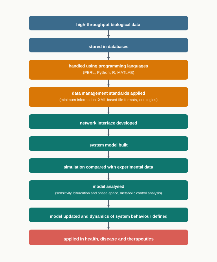
Fig. 11.7 – Chapter overview.
11.4 Key Terms
High-throughput — The handling of a very large number of samples, molecules or measurements automatically in one go, instead of one at a time by hand.
Artificial intelligence (AI) — Computer methods that carry out tasks which would otherwise need human reasoning, such as recognising patterns and making predictions.
Machine learning (ML) — A set of techniques in which a program learns patterns from large training data and then makes predictions on new data.
High level language — A programming language written in words and symbols close to ordinary human language, which the computer translates into its own machine instructions.
Operating system (OS) platform — The basic software environment, such as Linux, unix, mac or windows, on which other programs are developed and run.
Linux — The operating system platform on which the majority of successful bioinformatics applications have been developed.
PERL — A programming language that has been at the core of sequence-based large data handling since the beginning of bioinformatics.
Cloud computing — An arrangement in which the analysis actually runs on remote high-capacity machines rather than on the user’s own computer.
Python — A high level, general purpose, object oriented and interactive programming language created by Guido van Rossum (1991), widely used for sequence and structure analyses and phylogenetics.
Object oriented programming — A style of programming in which data and the operations on that data are bundled together into single units called objects.
Library — A ready-made, tested collection of code that a programmer can use instead of writing the same routine again.
R — A functional programming language named after its inventors Robert Gentleman and Robert Ihaka, ideal for high volume analysis, visualisation and simulation of biological data.
Free and open source — Software that anyone may use, and whose underlying code anyone may read and modify.
MATLAB — A computing platform that also provides a very good environment for bioinformatics data analysis and systems modelling.
GEC (Genetic Engineering of living Cells) — A rule based language developed by Microsoft for designing biological systems rather than only analysing data.
Kera — An object oriented, knowledge based programming language developed by Dr. Umesh P. of University of Kerala, which captures information on the genome, proteins and the cell.
Samhita — The user edited biological library through which the Kera language stores its biological knowledge.
Database — An organised digital storehouse in which biological data are labelled, indexed and made searchable by a computer.
In-vitro — An experiment carried out outside the living body, in glassware or culture.
In-vivo — An experiment carried out inside a living organism.
System model — A mathematical and computational representation of a biological system, built so that it behaves like the real system does in experiments.
Systems biology — An interdisciplinary field of study that focuses on complex biological interactions within biological systems by building and analysing system models.
Emergent functional property — A property that belongs to a whole system but to none of its individual components on their own.
Metabolic network — A system model of the interconnected reactions of metabolism, and one of the most efficient kinds of systems model.
Signaling network — A system model of the interconnected steps by which a cell receives and passes on signals.
Reductionist approach — The approach that studies a system by identifying and examining its individual components and interactions one at a time.
Pluralism — The many-sidedness of a living system, in which many components act and influence one another simultaneously.
Object network mapping — Representing every component of a system as an object and every influence between them as a link, producing a network that can then be integrated with dynamic events.
Network interface — The precise, mechanism-based description of how the components of a system act on one another, from which the model is developed.
Minimum information — The set of essential supporting information needed from an experiment so that its data can be interpreted and reused by others.
Metadata — Data about the data, such as the organism, instrument, conditions and settings of an experiment.
Extensible Markup Language (XML) — The kind of tagged file format in which systems biology data are generally stored, allowing automatic processing by computers.
Ontology — An agreed vocabulary that defines the meaning of each term used to annotate data, together with the hierarchical relationships between those terms.
Gene Ontology (GO) — A widely used ontology for annotating genes and their products.
Systems Biology Ontology (SBO) — An ontology developed for annotating the terms used in systems biology models.
Electronic lab notebook (ELN) — A web-based data-management system in which laboratory records are kept digitally.
Laboratory information management system (LIMS) — A data-management system that tracks samples, tests and results in a laboratory.
Workflow — A shareable computational pipeline that links several tools together, enabling data exchange, data integration and inter-tool communication.
Partial differential equations (PDEs) — Equations describing how a quantity changes with both time and position, used to represent spatiotemporal biological systems.
Finite Element Method (FEM) — A numerical technique that gives approximate solutions to partial differential equations by dividing the system into small elements.
Physiome — A large systems biology project aimed at a multi-scale modelling framework in which models can be combined and linked hierarchically.
Sensitivity analysis — A model-analysis method that describes the stability and controllability of a system against various disturbances.
Bifurcation and phase-space analysis — A model-analysis method used to discover the possible steady as well as dynamical tendencies of a system model.
Metabolic control analysis (MCA) — A model-analysis method that relates the properties of a metabolic network at steady state to its component reactions.
11.5 Points to Ponder
Hodgkin and Huxley solved their equations by hand on a mechanical calculator, and it took weeks. A laptop now does the same work in a fraction of a second. Has the speed of computation changed what biologists can discover, or only how quickly they discover it?
A programming language lets a scientist apply the same rule to millions of records without fatigue. But a mistake in that rule is also applied to all million records. What does this suggest about how carefully analysis code should be checked before it is trusted?
R is free and open source, while several equally powerful platforms are commercial products. If two laboratories reach different conclusions from the same data using different software, how would you go about deciding which result to believe?
Python is valued partly because its code is easy for another person to read. Why should the readability of code matter in science, when the computer would run an unreadable program equally well?
GEC and Kera were built for designing biological systems rather than for analysing data that already exist. What does it mean to “write” a living system in a programming language before it is ever built at the bench?
The Physiome project links models of ion channels, myofilament mechanics, tissue mechanics and coronary blood flow, each built by a different research group. What kinds of problems arise when scientific understanding has to be assembled from many independently made parts?
The reductionist approach identified genes, enzymes and receptors one at a time, and was extraordinarily successful. Why, then, could it not describe the pluralism of a living system — and does systems biology replace it, or depend on it?
An emergent property belongs to the whole system but to none of its parts. Can you think of an emergent property in an organism you have studied that could never be predicted by examining a single cell or a single molecule?
The Human Genome Project gave biology the complete list of parts for a human being. Why did having the full list make the need for systems biology greater rather than smaller?
A whole cell model of Mycoplasma genitalium could predict cell viability in response to genetic mutations. What would have to be true of our data before the same could be attempted for a human cell — and would a perfect model of a cell amount to understanding it?
The systems biology workflow is a loop, not a straight line: discrepancies between simulation and experiment are fed back into the model. Is a model that has been repeatedly adjusted to fit the data still capable of being disproved?
Minimum information, file formats and ontologies exist because different laboratories describe the same thing differently. Who should decide what these shared standards are, and what is lost when a laboratory has to abandon its own way of recording data?
Sensitivity analysis can show that a model’s behaviour depends heavily on one parameter. Should such a finding be treated as a discovery about biology, or as a warning about the model?
Systems biology is being applied to health and disease using data pooled from many patients. How far should individual patients be able to control what happens to their genomic data once it has entered such a model?
The chapter says the theme of systems biology is ‘object network mapping and its integration with interdependent dynamic events’. Try restating this in your own words for a classmate who has never heard the phrase, and see which part is hardest to explain.
11.6 NCERT Questions
Why are programming languages a boon for biologists?
Name the various aspects of data management for systems biology.
Choose the INCORRECT statement
- Python is a programming language.
- Biologists do not require knowledge of statistical tools for handling datasets.
- Most of the applications have been developed on Linux platform.
- Python provides third-party toolkits.
Systems biology is
- the systematic study of all the living organisms.
- the thorough study of all biochemical and signaling pathways.
- the detailed study of biological systems through computational and experimental methods.
- the study of dynamics of enzymes.
Which of the following is NOT included in data management systems?
- Metabolic control analysis
- Spreadsheets
- Web-based electronic lab notebooks (ELN)
- Laboratory information management systems (LIMS)
What is the need of systems biology?
What is the fundamental difference between systems biology and physiology?
Explain systems biology as collection of approaches and tools.
Is systems biology cell-centric?
11.7 Objective Questions
Python was created by
- Robert Gentleman
- Guido van Rossum
- Ludwig von Bertalanffy
- Mihajlo Mesarovic
The name of the R language has been derived from
- the word “research”
- its two inventors, Robert Gentleman and Robert Ihaka
- the Linux platform on which it was written
- the word “reductionist”
The majority of successful bioinformatics applications have been developed on
- the Windows platform
- the Mac platform
- the Linux platform
- cloud platforms only
Which language has been at the core of sequence-based large data handling from the beginning of bioinformatics?
- PERL
- MATLAB
- Kera
- GEC
Python has been successfully used for all of the following EXCEPT
- sequence analysis
- structure analysis
- phylogenetics
- solving partial differential equations by the Finite Element Method
Which of the following is a rule based language developed by Microsoft for designing living cells?
- Kera
- GEC
- BANJO
- Galaxy
Kera uses a user edited biological library called
- Physiome
- CytoSolve
- Samhita
- SimBoolNet
Mathematical and computational models built to mimic complex biological systems are called
- ontologies
- system models
- workflows
- metadata
In 1952, a mathematical model for action potential propagation along the axon of a neuronal cell was described by
- Denis Noble
- Mihajlo Mesarovic
- Alan Lloyd Hodgkin and Andrew Fielding Huxley
- Robert Gentleman and Robert Ihaka
The first computer model of the heart pacemaker, developed in 1960, is credited to
- Ludwig von Bertalanffy
- Denis Noble
- Guido van Rossum
- Andrew Fielding Huxley
Systems biology was formally launched in 1966 at the Case Institute of Technology, Cleveland, Ohio, by
- Ludwig von Bertalanffy
- Mihajlo Mesarovic
- Denis Noble
- Alan Lloyd Hodgkin
The whole cell model developed in 2012 at Mount Sinai School of Medicine, New York, was built for
- Escherichia coli
- Mycoplasma genitalium
- Agrobacterium tumefaciens
- Saccharomyces cerevisiae
The organism used for the 2012 whole cell model is described as
- a cell wall less bacterium
- a spore-forming bacterium
- a filamentous fungus
- a virus
The three basic aspects considered for data management in systems biology are
- storage, transfer and visualisation
- minimum information, file formats and ontologies
- curation, simulation and model analysis
- synthesis, analysis and modelling concept
File formats used for storing systems biology data are generally based on
- HTML
- XML
- PERL
Gene Ontology (GO) and Systems Biology Ontology (SBO) are examples of
- simulation tools
- data-management systems
- ontologies
- workflow engines
Which of the following allows the construction, execution and sharing of specialised workflows?
- Konstanz Information Miner (KNIME)
- MetNetMaker
- AutoDock Vina
- XPPAut
Partial differential equations used in systems modelling are solved by
- the Finite Element Method
- metabolic control analysis
- semantic annotation
- deep curation
Which model-analysis method describes the stability and controllability of a system against various disturbances?
- Bifurcation analysis
- Sensitivity analysis
- Metabolic control analysis
- Phase-space annotation
MetNetMaker is a tool used for
- sensitivity analysis
- bifurcation and phase-space analysis
- metabolic control analysis
- molecular docking
Which of the following is used in Table 11.1 under the facility “Molecular interaction”?
- COBRA
- AutoDock Vina
- PathVisio
- MAGE-TAB
The Physiome project is aimed at developing
- a single model of one bacterial cell
- a multi-scale modelling framework in which models can be combined hierarchically
- a new programming language for gene design
- a database of restriction enzymes
Examples of the most efficient system models given in the chapter are
- metabolic and signaling networks
- spreadsheets and lab notebooks
- ontologies and file formats
- sequence and structure datasets
Assertion (A): The majority of successful bioinformatics applications have been developed on the Linux platform. Reason (R): Bioinformatics software cannot be developed for any other operating system platform.
Assertion (A): Python is very popular within the bioinformatics community. Reason (R): Python offers clear terms and statement structure, alignment to object-oriented programming, and a wide availability of libraries and third-party toolkits.
Assertion (A): The R language is widely used for high volume analysis and visualisation of biological data. Reason (R): R was developed as a rule based language for designing genetic circuits in living cells.
Assertion (A): Systems biology is described as an interdisciplinary field of study. Reason (R): It draws upon life science, information science and system science together.
Assertion (A): The reductionist approach could not convincingly describe the pluralism of a biological system. Reason (R): Pluralism can be observed only through quantitative measures of multiple components simultaneously, which requires mathematical models with rigorous data integration.
Assertion (A): Metadata must be incorporated along with the data collected in a systems biology experiment. Reason (R): Without supporting information about how and under what conditions the data were obtained, the data cannot be correctly interpreted or reused by others.
Assertion (A): Ontologies are needed even after data have been stored in a common file format. Reason (R): A file format fixes how the data are written, whereas an ontology fixes what the terms describing the data actually mean.
Assertion (A): In a systems biology experiment, the simulation is repeated and tested again and again. Reason (R): Discrepancies between model-based simulation results and experimental data are used to remodel the hypothesis and update the model.
Assertion (A): The network interface transferred for model development should be mechanism based. Reason (R): A model built only on correlations between components cannot reliably predict the behaviour of the system under new conditions.
Assertion (A): The Human Genome Project is regarded as one of the seedings of the thought of systems biology. Reason (R): Once the complete list of components became available, the outstanding problem shifted to explaining how those components work together.
11.8 Check Your Concepts
The data from an experiment have already been generated by the machine. Why, then, is a programming language still needed before any biological conclusion can be drawn?
The chapter lists five challenges brought by massive data — storage, visualisation, transfer, analysis and interpretation. Explain, in one sentence each, why every one of these is a genuine difficulty and not merely an inconvenience.
Why is the readability of code considered an advantage of Python in the bioinformatics community, when a computer would execute badly written code equally well?
A student says, “Python and R do the same thing, so learning one is enough.” Evaluate this statement using the specific strengths and typical biological uses of each language.
Explain why a language built for text and pattern matching, such as PERL, became central to sequence-based large data handling.
State two practical reasons why the majority of successful bioinformatics applications have been developed on the Linux platform.
GEC and Kera are grouped separately from Python and R in this chapter. On what basis are they separated, and what does each group of languages set out to do?
What is meant by a “user edited biological library”, and what advantage does this design give to a knowledge based language such as Kera?
Match the following:
| Column I | Column II |
|---|---|
| a. Guido van Rossum | i. First theory about systems biology |
| b. Robert Gentleman and Robert Ihaka | ii. First computer model of the heart pacemaker |
| c. Denis Noble | iii. Python |
| d. Ludwig von Bertalanffy | iv. Formal launch of systems biology in 1966 |
| e. Mihajlo Mesarovic | v. R |
- Match each facility with the software listed against it in the chapter:
| Column I (Facility) | Column II (Tool) |
|---|---|
| a. Curation | i. BANJO |
| b. Network inference | ii. AutoDock Vina |
| c. Molecular interaction | iii. PathVisio |
| d. Physiological modelling | iv. MAGE-TAB |
| e. Data management | v. PhysioDesigner |
Arrange the following in correct chronological order, and state briefly what each contributed: first computer model of the heart pacemaker; whole cell model of Mycoplasma genitalium; mathematical model of action potential propagation; first published theory about systems biology; formal launch of systems biology.
Arrange the steps of a standard systems biology experiment in their correct sequence: development of the network interface; definition of the problem; analysis of discrepancies between simulation and experiment; arrangement of data in appropriate file formats; execution of the experiment; designing of the experiment; incorporation of new hypotheses into the model; model development.
Draw the diagram depicting systems biology as an interdisciplinary field and label its three sectors along with the three items listed inside each.
In the workflow for a systems biology experiment, the final arrow returns to an earlier step rather than ending the process. Explain why the workflow is drawn as a loop, and what would be lost if it were carried out only once.
A research group develops a network interface that records which pairs of proteins rise and fall together, but not how one protein acts upon the other. What condition of the protocol has been violated, and what will go wrong when the resulting model is used to predict behaviour under new conditions?
A laboratory uploads its microarray results as plain numbers, without recording the organism, the instrument settings or the date of the experiment. Identify which aspect of data management has been neglected, and explain what happens when another group tries to reuse those data.
Two laboratories store their data in the same XML-based file format, yet a computer still cannot combine their results meaningfully. Which aspect of data management is missing, and how does it solve the problem?
Distinguish between minimum information, file formats and ontologies, giving the specific role of each in systems biology data management.
Compare the reductionist approach and the systems approach with respect to the question asked, the method used, and the main limitation of each.
Physiology and systems biology both study how living systems function. Explain how the level of description and the tools used differ between the two.
What is an emergent functional property? Give one example from the chapter and explain why the property disappears when the system is studied component by component.
Explain the statement: “Systems biology is the observation of a system by integrating different components together.” Why can pluralism not be described by measuring one component at a time?
Break the phrase “object network mapping and its integration with interdependent dynamic events — kinetics with partial differential equations” into its three parts and explain each in simple language.
Why are partial differential equations, rather than ordinary equations, used to represent spatiotemporal biological systems? What does the Finite Element Method do with them?
The whole cell model of 2012 was built for an organism with a very small genome. Explain why this choice made the task feasible, and what additional difficulties a whole cell model of a human cell would face.
The Physiome project links models of ion channels, myofilament mechanics, tissue mechanics and coronary blood flow. Why does combining models built by different research groups require agreed standards for data management?
A model of a signalling pathway reproduces the experimental data perfectly. A colleague argues that no further testing is required. Using the three model-analysis methods described in the chapter, explain why this argument is unsatisfactory.
For each situation below, name the model-analysis method that should be applied and justify your choice:
- A team wants to know which enzyme in a metabolic network, at steady state, exerts the greatest control over the pathway flux.
- A team wants to know whether their model will settle at a fixed level or begin to oscillate as one condition is varied.
- A team wants to know how far the model’s predictions shift when one measured parameter is slightly disturbed.
What happens to a systems biology model if the data feeding it are abundant but of poor quality? Relate your answer to the role of functional genomics since the 1990s in making more realistic models possible.
Explain how cloud computing makes genome-scale analysis possible for a researcher working on an ordinary laptop.
Why is the ability to share a workflow, and not merely to run it, considered important in systems biology research?
11.9 Case-Based Questions
A newly set up plant biotechnology laboratory installs a high-throughput sequencer. Within three months it has accumulated sequence files far larger than any computer in the department can open. A research scholar tries to search the files for a particular motif by scrolling through them by hand, and after two days has covered only a small fraction of the data. The head of the laboratory decides that every member of the group must learn at least one programming language, and that the analysis will be shifted to a Linux server with cloud access.
- Identify the specific challenges of massive data that this laboratory is facing.
- Explain why manual searching is unsuitable here, mentioning two advantages that a short program would offer over the scholar’s method.
- Suggest which language would suit sequence-based text handling and which would suit the statistical analysis of the results, giving a reason for each choice.
- State one reason why the group’s work was shifted to a Linux server rather than kept on individual desktop machines.
Two laboratories in different countries agree to pool their proteomics results. Laboratory A stores its data as a spreadsheet with column headings of its own invention, and does not record the instrument settings used. Laboratory B stores its results in an XML-based format with full experimental details, and annotates every protein using a standard vocabulary. When the two datasets are handed to a programmer for combined analysis, the software reads Laboratory B’s files automatically but fails completely on Laboratory A’s, and even after manual correction, several entries in the two sets cannot be matched to one another.
- Which aspect of data management has Laboratory A neglected in not recording its instrument settings, and what is the general name for such supporting information?
- Explain why the software could process Laboratory B’s files automatically.
- Even after the formats are made identical, some entries still cannot be matched. Which third aspect of data management addresses this, and name two examples of it given in the chapter.
- Suggest what the two laboratories should have agreed upon before beginning their collaboration.
A systems biology group defines a problem concerning a bacterial signalling pathway, designs and executes experiments, arranges the resulting data in appropriate file formats, and develops a network interface from which a model is built. When the model is simulated, the predicted level of one signalling protein is roughly half of what the experiments actually show. One member of the group suggests discarding the model as a failure. The supervisor instead asks the group to examine the disagreement carefully, remodel the hypothesis and simulate again.
- Arrange the steps the group has already completed in their correct order, as followed in a standard systems biology experiment.
- Explain why the supervisor treats the discrepancy as useful rather than as a failure.
- What is likely to be missing from the network interface if a component’s predicted level is consistently wrong?
- Describe what the group should do after the hypothesis has been remodelled.
A computational biology team wishes to predict whether a bacterial cell will survive when a particular gene is deleted. Rather than performing hundreds of knockout experiments at the bench, they use a whole cell model of an organism whose genome is among the smallest known for a free-living cell. The model brings together all the known molecular processes of that cell, and can be asked what will happen under mutations that have never been tested experimentally.
- Name the organism for which such a whole cell model was developed, the year, and the institution credited with it.
- Why was an organism with a very small genome chosen for the first attempt at a whole cell model?
- State one clear advantage and one clear limitation of predicting cell viability by simulation instead of by experiment.
- If the model predicts that a deletion is lethal but the bench experiment shows that the cell survives, what should the team conclude?
A metabolic engineering team wants to increase the yield of a valuable compound produced by a cultured cell line. They build a model of the metabolic network and, at steady state, systematically alter the activity of each enzyme in turn to see how the flux through the pathway responds. They find that altering one particular enzyme changes the output substantially, while altering three others changes it hardly at all. A junior member proposes that the team should also check whether the model’s behaviour changes qualitatively as the supply of the starting substrate is increased.
- Name the model-analysis method the team has used, and state the relationship it is designed to reveal.
- Explain what the team should conclude about the enzyme whose alteration changed the output substantially.
- What older idea about the control of a pathway does this method replace, and how?
- Name the model-analysis method appropriate to the junior member’s suggestion, and state what it would show.
A hospital research centre is building a systems biology model of a heart disorder. The model links ion channel behaviour and signal transduction at the subcellular level with tissue mechanics and coronary blood flow at the organ level, drawing on models built by four separate research groups. To make the model clinically useful, the centre proposes to train it on genome sequences and clinical records pooled from several thousand patients. The ethics committee raises objections before granting approval.
- Name the large systems biology project whose approach the centre is following, and state what kind of modelling framework it aims to develop.
- Explain why combining models made by four different groups requires agreed data-management standards.
- State two arguments in favour of building such a model from real patient data, and two concerns the ethics committee is likely to have raised.
- Suggest two safeguards the committee could insist upon before the pooled data are used.