Chapter 1: Electric Charges and Fields
Around 600 BC, in the Greek city of Miletus, a philosopher named Thales noticed something strange. When he rubbed a piece of amber — a hard, yellowish fossilized tree resin — against wool or fur, the amber began to attract light objects like bits of straw, dry leaves, and feathers. The amber had not been heated, glued, or magnetized. It simply pulled these objects toward itself after being rubbed. To Thales and those around him, this looked almost like magic.
That single observation, made more than two and a half thousand years ago, was the first recorded step toward understanding electricity. In fact, the very word “electricity” comes from elektron, the Greek word for amber. For centuries, no one could explain what invisible influence the rubbed amber carried, or why it faded away when the amber touched certain objects.
Today we recognize this “amber effect” as the everyday phenomenon of static electricity — the same thing that makes your hair rise when you remove a sweater, or gives you a small shock when you touch a metal door handle in dry weather. Behind all of it lies a fundamental property of matter called electric charge, and a way in which charges reach out across empty space to influence one another: the electric field.
This chapter builds the foundation for everything you will study about electricity. We begin exactly where Thales did — with rubbing, attraction, and a puzzle.
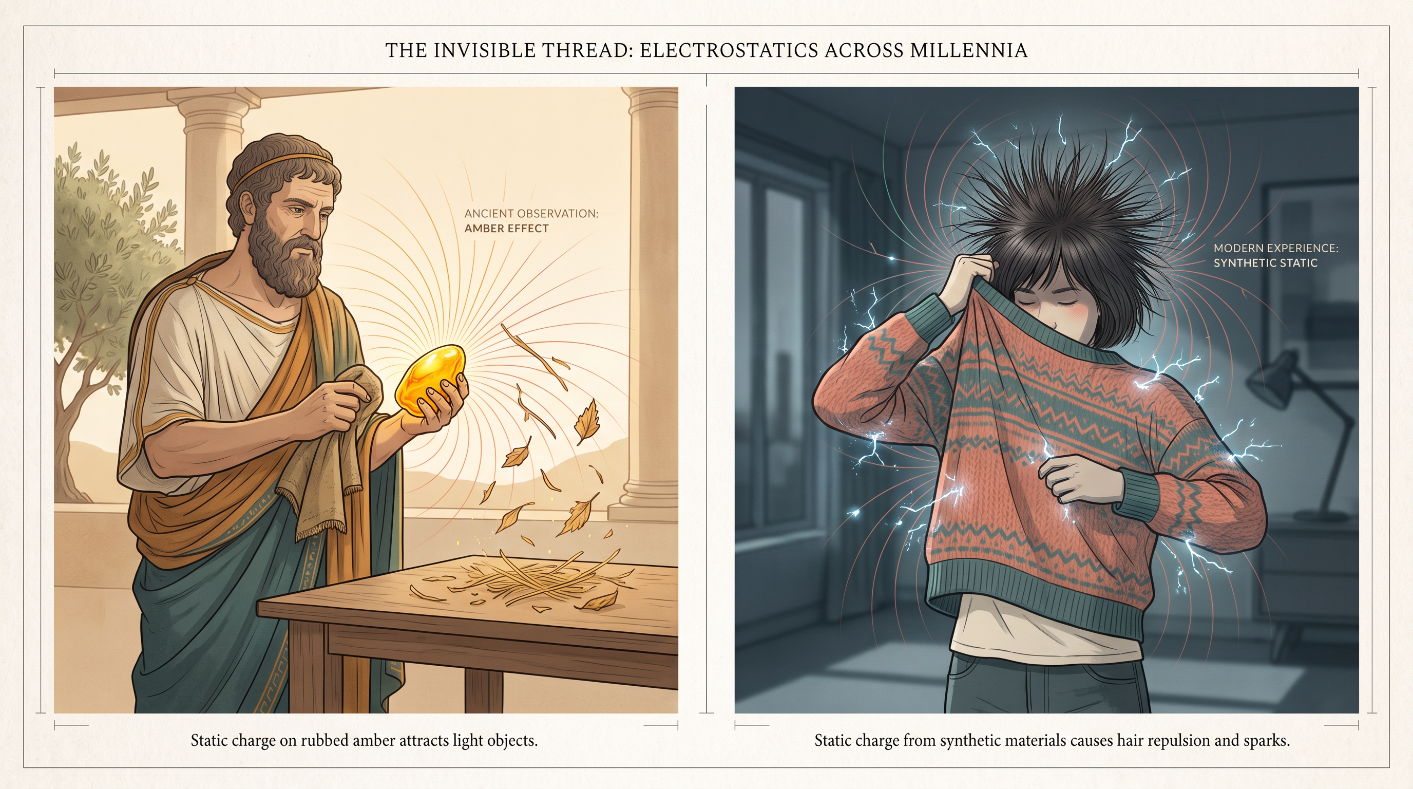
Fig. 1.0 – Ancient and modern examples of static electricity.
By the end of this chapter, you will be able to answer each of these questions using a small set of powerful ideas: electric charge, Coulomb’s law, the electric field, and Gauss’s law.
1.1 Introduction
Think about the last time you pulled off a sweater made of synthetic material on a cold, dry day. You may have heard a faint crackling sound, and in a dark room you might even have seen tiny sparks jumping between the cloth and your skin. Many of us have felt this without ever asking why it happens.
The same kind of thing shows up in other everyday moments. When you step out of a car and touch its metal door, you sometimes feel a sudden, small electric shock. The same shock can happen when you grab the metal handrail of a bus after sliding across your seat. These little jolts are surprisingly common, especially when the air is dry.
Nature shows us a far more dramatic version of the same effect. The lightning that flashes across the sky during a thunderstorm is also a form of electric discharge — the same basic process as the tiny spark from your sweater, but on an enormous scale.
So what links a crackling sweater, a shock from a car door, and a bolt of lightning? In every case, electric charges have quietly built up on a surface, and then suddenly flowed away — through your body, through the air, or through some other path. That sudden flow of built-up charge is what we call an electric discharge.
Where do these charges come from in the first place? They are produced when two surfaces — often insulating surfaces like cloth, plastic, or rubber — rub against each other. This rubbing transfers charge from one surface to the other, leaving each surface electrically charged. Because this charge tends to stay put rather than move around, the effect is known as static electricity.
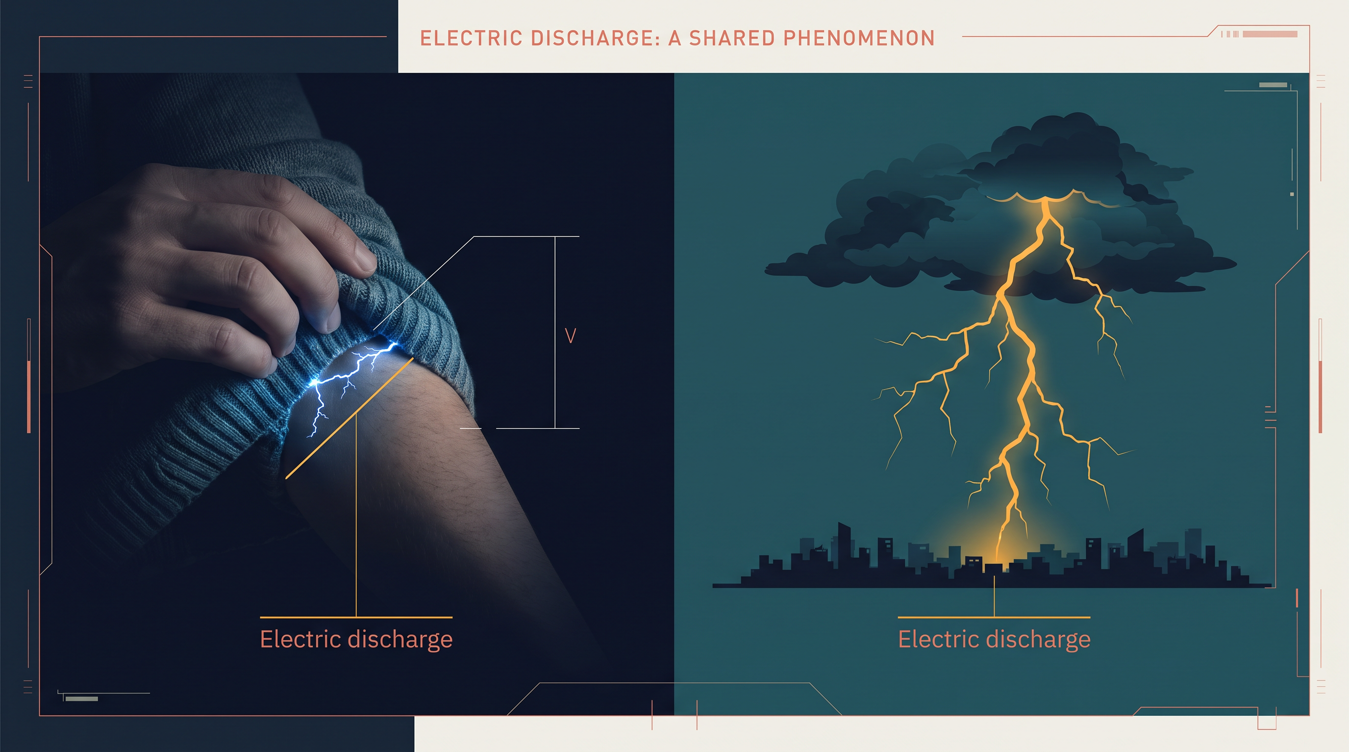
Fig. 1.1 – Electric discharge in everyday life and in nature.
The word “static” simply means something that does not move or change with time. Here it refers to charges that are essentially at rest on a surface, held in place until a path lets them escape. This branch of physics — the study of charges that are not moving, and of the forces, fields, and potentials they produce — is called electrostatics.
This chapter, and the next, are devoted to electrostatics. Here we will build up the basic ideas step by step: what electric charge is, how charges exert forces on one another, how a charge fills the surrounding space with an electric field, and how a powerful rule called Gauss’s law lets us calculate that field in symmetric situations. Everything begins with the simple, familiar observation that rubbed objects can attract, repel, and shock — and with the question of what invisible property makes them do so.
1.2 Electric Charge
In the chapter opener we saw that rubbed amber attracts light objects, and that this is where the very word “electricity” comes from. But this is only one example out of many. Over the centuries, people found that a large number of material pairs behave in the same way — when rubbed together, they gain the ability to attract light things like straw, pith balls, and small bits of paper.
Let us look more carefully at what happens when different objects are rubbed and then brought near one another. These simple experiments, repeated and refined over many years, hold the key to the whole idea of electric charge.
Rubbing experiments
Suppose you rub two glass rods with wool or silk cloth and then bring them close together. Instead of attracting, the two rods push each other away — they repel. Interestingly, the two pieces of cloth used to rub them also repel each other. But each glass rod attracts the cloth that rubbed it. This is shown in Fig. 1.2(a).
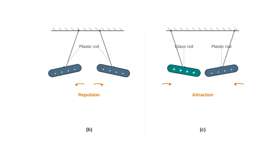
Fig. 1.2(a) – Repulsion between two positively charged glass rods.
Now try the same with plastic rods rubbed using cat’s fur. The two plastic rods repel each other, but each attracts the fur that rubbed it, as in Fig. 1.2(b). And when you bring a rubbed plastic rod near a rubbed glass rod, the two attract each other, as in Fig. 1.2(c). The plastic rod repels the silk or wool, while the glass rod repels the fur.
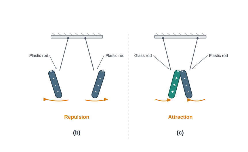
Fig. 1.2(b) and (c) – (b) Repulsive force between plastic rods and (c) attractive force between a plastic and a glass rod.
These may look like small, scattered facts, but scientists studied them patiently for years. A clear pattern finally emerged from all this careful work.
Two kinds of charge
The conclusion was striking in its simplicity: there are only two kinds of electric charge in nature. When objects like glass rods, plastic rods, silk, fur, or pith balls are rubbed, they become electrified — that is, they acquire an electric charge. And these charges behave in just two ways.
Objects carrying the same kind of charge push each other apart, while objects carrying different kinds of charge pull toward each other. In short: like charges repel, and unlike charges attract.
The property that tells the two kinds of charge apart — that decides whether two charged bodies will attract or repel — is called the polarity of charge.
Positive and negative: naming the charges
Here is a revealing observation. When a glass rod is rubbed with silk, the rod gains one kind of charge and the silk gains the other kind. This happens for every such pair of objects rubbed together. Now, if you bring that same electrified glass rod back into contact with the silk that rubbed it, they no longer attract each other. They also lose their power to attract or repel other light objects.
In other words, the charges the two bodies gained during rubbing are cancelled out when the bodies are brought together again. This tells us something important: the two kinds of charge neutralise, or nullify, each other’s effect.
Because the two kinds of charge oppose and cancel each other, it was natural to label one kind as positive and the other as negative. This naming convention was introduced by the American scientist Benjamin Franklin.
By convention, the charge appearing on a glass rod (or on cat’s fur) is called positive, and the charge on a plastic rod (or on silk) is called negative. An object that carries any electric charge is said to be electrified or charged. An object with no net charge is said to be electrically neutral.
Detecting charge: the gold-leaf electroscope
How do we actually detect whether a body is charged, and roughly how much charge it carries? A simple instrument for this is the gold-leaf electroscope, shown in Fig. 1.3(a).
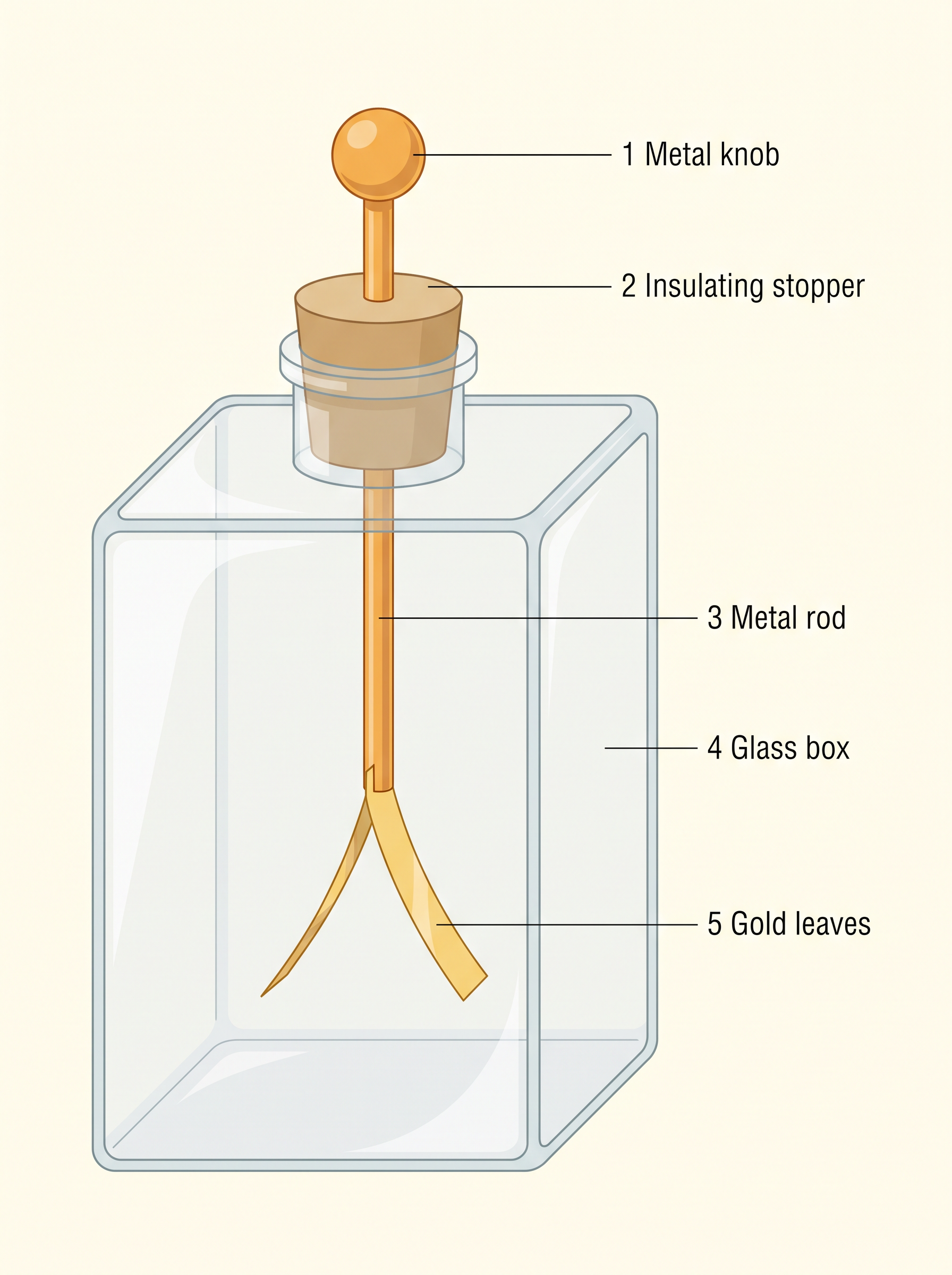
Fig. 1.3(a) – A gold-leaf electroscope.
It consists of a vertical metal rod enclosed in a box, with two thin gold leaves attached to the lower end of the rod. When a charged object touches the metal knob at the top, charge flows down the rod and onto the leaves. Since both leaves now carry the same kind of charge, they repel each other and spread apart, or diverge. The greater the amount of charge transferred, the wider the leaves diverge — so the amount of divergence indicates how much charge is present.
Why do rubbed bodies acquire charge?
To understand where this charge comes from, recall that all matter is made up of atoms and molecules. Normally, materials are electrically neutral — but this does not mean they contain no charges. In fact, they contain a great many positive and negative charges; it is just that these charges are exactly balanced, so there is no net charge.
This inner electrical nature of matter is far-reaching. The forces that hold molecules together, that bind atoms inside a solid, the adhesive force of glue, and even the forces of surface tension are all basically electrical in origin — they arise from the forces between charged particles. In this sense, the electric force is all-pervasive, touching almost every aspect of the physical world around us.
To electrify a neutral body, we must upset this balance by adding or removing one kind of charge. So when we say a body is “charged,” we always mean it has an excess of one kind of charge or a deficit of it.
In solids, some of the electrons — being less tightly bound to their atoms — are the charges that can move from one body to another. A body becomes positively charged by losing some of its electrons, and negatively charged by gaining extra electrons.
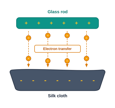
Fig. 1.4 – Electron transfer between a glass rod and a silk cloth.
This is exactly what happens during rubbing. When a glass rod is rubbed with silk, some electrons are transferred from the rod to the silk cloth. The rod, having lost electrons, becomes positively charged, and the silk, having gained them, becomes negatively charged. No new charge is created in this process — charge is only moved from one body to the other. Also, the number of electrons actually transferred is an extremely small fraction of the total number of electrons in the material.
1.3 Conductors and Insulators
We have seen that rubbing can transfer charge from one body to another. But what happens to that charge once it is on a body? The answer depends very much on the material — because some materials let charge move around freely, while others hold it firmly in place.
Some substances allow electricity to pass through them easily. These are called conductors. Inside a conductor, some of the electric charges — in particular, the electrons — are comparatively free to move about within the material. Because these charges can travel through the substance, they carry electricity from one point to another.
Metals are the most familiar conductors. Copper, aluminium, iron, and silver all conduct electricity well. Perhaps more surprisingly, the human body and other animal bodies are also conductors, and so is the earth itself.
Other substances resist the passage of electricity. Most non-metals — such as glass, porcelain, plastic, nylon, and wood — offer high resistance to the flow of charge through them. These are called insulators. In an insulator, the charges are not free to move, so electricity cannot easily pass through.
Most substances fall into one of these two classes — either conductor or insulator. However, there is also a third, in-between category. Some materials, called semiconductors, offer a resistance that lies between that of conductors and insulators. They neither conduct as freely as metals nor block charge as completely as insulators, and this intermediate behaviour makes them extremely important in modern electronics.
How conductors and insulators handle charge
There is an important difference in how the two kinds of material deal with charge given to them. When some charge is transferred to a conductor, that charge quickly spreads out and distributes itself over the entire outer surface of the conductor. This happens because the free charges repel one another and move apart until they are spread across the surface.
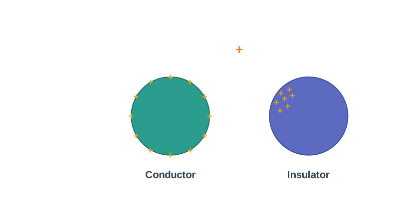
Fig. 1.5 – Distribution of charge on a conductor and an insulator.
In contrast, when charge is placed on an insulator, it stays at the same place where it was put. Since the charges cannot move, they do not spread out. (You will learn the deeper reason for this behaviour in the next chapter.)
A familiar puzzle: comb versus spoon
This conductor–insulator difference explains a common observation. Run a nylon or plastic comb through dry hair, or rub it, and it becomes electrified — it can then attract small pieces of paper. But rub a metal object such as a spoon in the same way, and it shows no sign of charging. Why the difference?
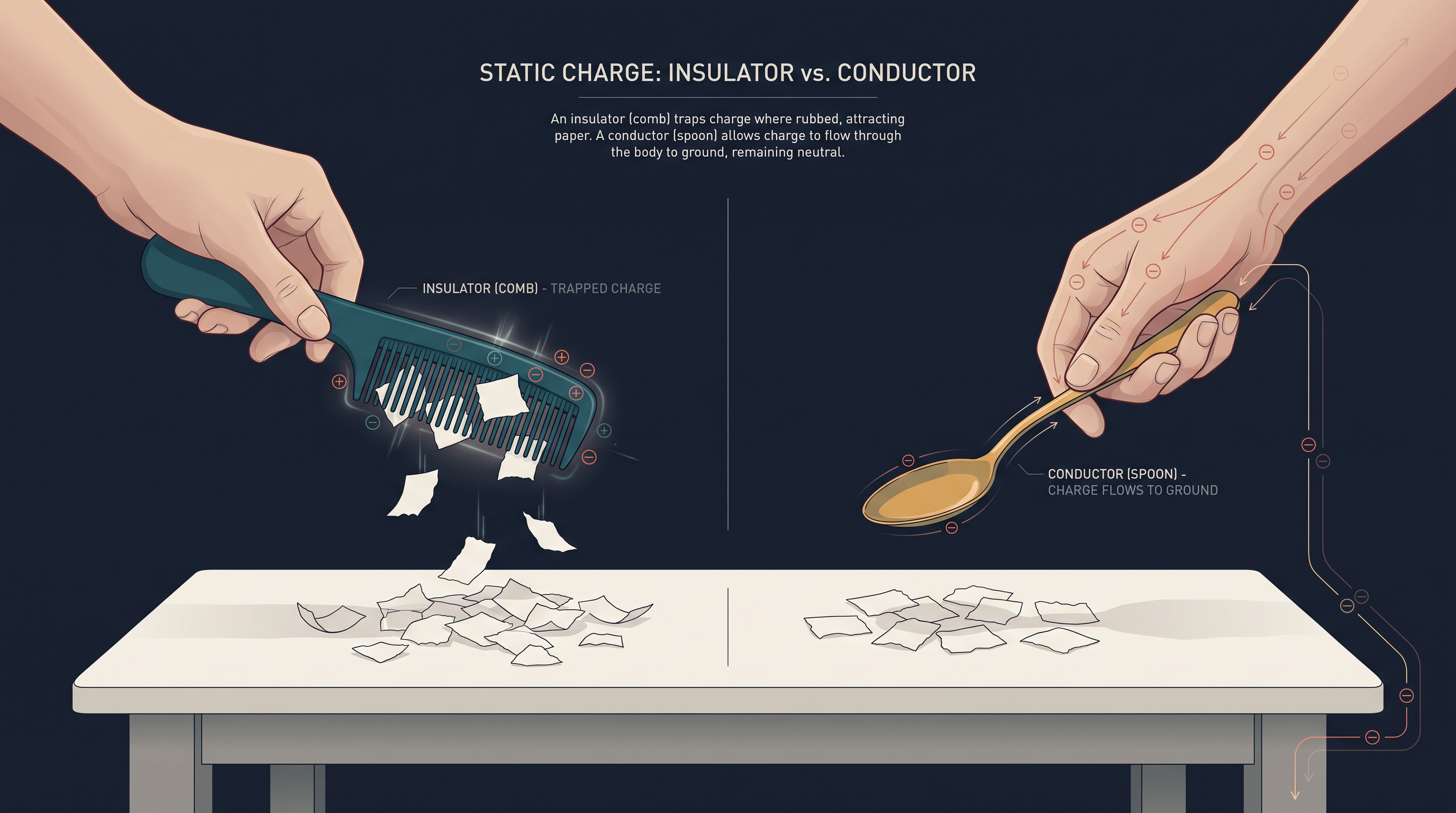
Fig. 1.6 – Charging an insulating comb versus a conducting spoon.
The comb is an insulator, so any charge it gains during rubbing stays on it. The spoon, however, is a metal conductor, and so is your body. Any charge that builds up on the spoon leaks away through your hand and body to the ground, because your body and the earth form a conducting path. The charge escapes as fast as it is produced, so the spoon never appears charged.
There is a neat way to confirm this explanation. If you take a metal rod fitted with a wooden or plastic handle and rub the rod without touching its metal part, the rod does show signs of charging. The insulating handle blocks the escape route to your body, so the charge is trapped on the metal and stays there.
1.4 Basic Properties of Electric Charge
So far we know that there are two types of charge — positive and negative — and that their effects tend to cancel each other. But charge has several other important properties that we now need to describe carefully. These properties will be used again and again throughout electrostatics.
Before listing them, it helps to introduce a simplifying idea. In many situations, the charged bodies we deal with are very small compared to the distances separating them. When this is true, the actual size and shape of the body no longer matter, and we can imagine all of its charge as being concentrated at a single point in space. Such an idealised charge is called a point charge.
Treating charges as point charges makes the mathematics far simpler, and it is a very good approximation whenever the charges are far apart relative to their own dimensions. With this idea in hand, we can now look at three basic properties of electric charge: additivity, conservation, and quantisation.
1.4.1 Additivity of charges
The first property concerns how the charges in a system combine. We have not yet given a precise quantitative definition of charge — that will come in the next section, when we discuss Coulomb’s law. For now, let us simply assume that charge can be measured as a number, and proceed.
Suppose a system contains two point charges, \(q_1\) and \(q_2\). The total charge of the system is found by simply adding the two charges together, taking their signs into account. That is, charges add up like ordinary real numbers. This is what we mean when we say charge is a scalar quantity — much like mass, it has magnitude but no direction.
If a system contains \(n\) charges \(q_1, q_2, q_3, \ldots, q_n\), then the total charge of the system is
\[q = q_1 + q_2 + q_3 + \cdots + q_n\]
where each \(q_i\) is included with its own sign, and the total charge \(q\) is measured in coulombs (C).
There is one key difference between charge and mass. Mass is always positive, but charge can be either positive or negative. So when adding charges, we must be careful to use the correct sign for each one.
For example, suppose a system contains five charges \(+1\), \(+2\), \(-3\), \(+4\), and \(-5\), in some arbitrary unit. The total charge is
\[(+1) + (+2) + (-3) + (+4) + (-5) = -1\]
in the same unit — not the simple count of “five charges,” but the signed sum.
1.4.2 Charge is conserved
The second property is one of the most important conservation laws in physics. We have already seen that when bodies are charged by rubbing, electrons are simply transferred from one body to the other — no new charge is created, and none is destroyed.
This idea can be stated more generally. When we rub two bodies together, whatever charge one body gains, the other body loses by exactly the same amount. Even inside a complicated system of many charged bodies, the charges may shift and redistribute themselves through their interactions, but the total charge of the isolated system stays exactly the same. This fact, confirmed by many experiments, is called the conservation of charge.
Here we must be careful about what exactly is conserved. It is the net charge of an isolated system that cannot be created or destroyed. The charge-carrying particles themselves, however, can be created or destroyed in certain processes — as long as the total charge does not change.
Nature provides a striking example. Sometimes a neutron transforms into a proton and an electron. Two brand-new charged particles appear where there were none before. But the proton carries charge \(+e\) and the electron carries charge \(-e\), so their charges are equal and opposite. The total charge is zero both before the neutron decays and after — so charge is still conserved, even though new charged particles have been created.
1.4.3 Quantisation of charge
The third property tells us that charge does not come in arbitrary amounts. Experiments have established that every free charge is a whole-number multiple of a certain basic, smallest unit of charge, denoted by \(e\). This means the charge \(q\) on any body can always be written as
\[q = ne\]
where \(n\) is any integer — positive, negative, or zero — and \(e\) is the basic unit of charge in coulombs (C).
This basic unit \(e\) is the amount of charge carried by a single electron or a single proton. By convention, the electron’s charge is taken as negative, so we write the charge on an electron as \(-e\) and the charge on a proton as \(+e\).
The fact that electric charge always comes as an integer multiple of \(e\) is called the quantisation of charge.
There are many quantities in physics that are “quantised” in this way — allowed only in discrete steps rather than continuous amounts. Charge was one of the first.
The unit of charge
In the International System (SI) of units, charge is measured in a unit called the coulomb, written C. The coulomb is actually defined using electric current, which you will study later. In those terms, one coulomb is the amount of charge that flows through a wire in one second when the current is one ampere (1 A).
In this system, the measured value of the basic unit of charge is
\[e = 1.602192 \times 10^{-19} \ \text{C}\]
This is an extremely small number, which tells us the coulomb is a very large unit of charge. In fact, a charge of just \(-1\) C contains about \(6 \times 10^{18}\) electrons. Because everyday electrostatic charges are far smaller than a coulomb, we usually work with smaller units: the microcoulomb, \(1\ \mu\text{C} = 10^{-6}\) C, and the millicoulomb, \(1\ \text{mC} = 10^{-3}\) C.
Why charge is quantised
If protons and electrons are the only basic charges in the universe, then every observable charge must be a whole-number multiple of \(e\). To see why, imagine a body containing \(n_1\) electrons and \(n_2\) protons. Its total charge is
\[q = n_2 \times e + n_1 \times (-e) = (n_2 - n_1), e\]
Since \(n_1\) and \(n_2\) are both integers, their difference \((n_2 - n_1)\) is also an integer. So the charge on any body is always an integer times \(e\), and it can only be increased or decreased in steps of \(e\).
Why we usually don’t notice the steps
The step size \(e\) is so tiny that at the everyday, macroscopic level we never notice the “graininess” of charge. When we handle charges of a few microcoulombs, they contain such an enormous number of electronic charges that adding or removing one more electron makes no visible difference.
A helpful comparison is a dotted line. Viewed from far away, a dotted line looks like one continuous line, even though it is really made of separate dots. In the same way, a large charge looks perfectly continuous even though it is built from countless tiny units of \(e\).
Let us put numbers to this. Since \(e = 1.6 \times 10^{-19}\) C, a charge of just \(1\ \mu\text{C}\) contains something like \(10^{13}\) times the electronic charge. At this scale, the fact that charge changes only in units of \(e\) is practically the same as saying it can take any continuous value. So at the macroscopic level, quantisation of charge has no practical consequence and can be safely ignored.
The situation is completely different at the microscopic level. When the charges involved are only a few tens or hundreds of \(e\) — small enough to be counted individually — the charge clearly appears in discrete lumps, and quantisation cannot be ignored. It is the scale of the situation that decides whether quantisation matters.
It is also useful to know roughly how many electrons a small piece of material contains. A cube of copper of side 1 cm contains about \(2.5 \times 10^{24}\) electrons.
1.5 Coulomb’s Law
So far we have described charges qualitatively — as positive or negative, attracting or repelling. But physics needs numbers. How strong is the force between two charges, and how does it depend on the amount of charge and on the distance between them? The answer is given by Coulomb’s law, a precise quantitative statement about the force between two point charges.
Recall that when the size of the charged bodies is much smaller than the distance separating them, we can treat them as point charges, with all their charge concentrated at a point. Coulomb studied exactly this case. By careful measurement, he found how the force between two point charges depends on the charges and their separation.
What Coulomb found
Coulomb discovered two things about the force between two point charges. First, the force varies inversely as the square of the distance between the charges — double the distance, and the force drops to one-fourth. Second, the force is directly proportional to the product of the magnitudes of the two charges. And the force acts along the straight line joining the two charges.
Putting these together, if two point charges \(q_1\) and \(q_2\) are separated by a distance \(r\) in vacuum, the magnitude of the force \(F\) between them is
\[F = k\frac{|q_1 q_2|}{r^2} \tag{1.1}\]
Here \(F\) is the force in newtons (N), \(q_1\) and \(q_2\) are the two charges in coulombs (C), \(r\) is the distance between them in metres (m), and \(k\) is a constant of proportionality whose value we will fix shortly.
How Coulomb measured the force
Measuring such a tiny force was not easy. Coulomb used a sensitive instrument called a torsion balance to measure the force between two small charged metallic spheres. When the separation between the two spheres is much larger than the radius of each sphere, the spheres can be treated as point charges.
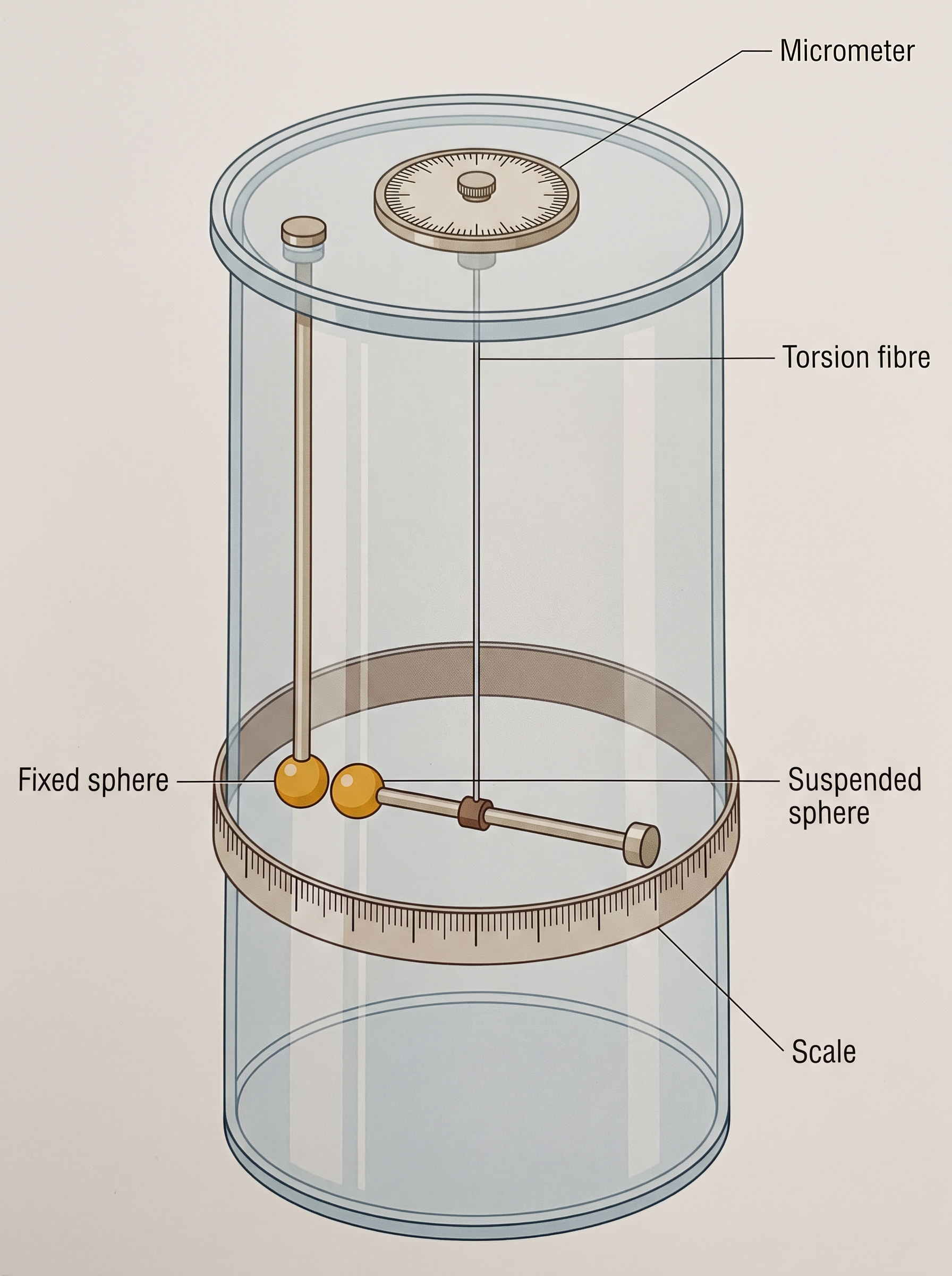
Fig. 1.7 – Coulomb’s torsion balance.
There was a clever difficulty Coulomb had to overcome: he did not know the actual amount of charge on his spheres. He got around this using a neat trick based on symmetry. Suppose a metallic sphere carries charge \(q\). If it is touched to an identical uncharged sphere, the charge spreads equally over both, so each ends up with \(q/2\). Repeating this, he could produce charges of \(q/2\), \(q/4\), and so on — known fractions of the original, even without knowing \(q\) itself.
Using these known ratios of charge, Coulomb first fixed a pair of charges and measured the force at several separations, confirming the inverse-square dependence on distance. Then he kept the distance fixed and varied the charges, confirming the dependence on the product of the charges. Combining both results gave Eq. (1.1).
Coulomb’s law began as an experimental result at the macroscopic scale. Remarkably, it has since been verified to hold even down to subatomic distances, of the order of \(r \sim 10^{-10}\) m.
Fixing the constant \(k\) and defining the coulomb
An interesting point is that Coulomb discovered his law without knowing the explicit size of the charges he was using. In fact, we can turn this around: Coulomb’s law can be used to define the unit of charge.
In Eq. (1.1), the constant \(k\) is so far arbitrary — we are free to choose any positive value for it. But the choice of \(k\) automatically fixes the size of the unit of charge. In SI units, the value of \(k\) is chosen to be about
\[k \approx 9 \times 10^{9} \ \frac{\text{N m}^2}{\text{C}^2}\]
The unit of charge that results from this choice is the coulomb (C), which we already introduced in Section 1.4. Putting this value of \(k\) into Eq. (1.1), and taking \(q_1 = q_2 = 1\) C with \(r = 1\) m, we get
\[F = 9 \times 10^{9} \ \text{N}\]
So we can now state precisely what one coulomb means: one coulomb is that charge which, when placed 1 m away from an equal charge in vacuum, experiences a repulsive force of \(9 \times 10^{9}\) N. This is a colossal force, which tells us that one coulomb is an extremely large unit of charge. In practice, we work with much smaller units such as the millicoulomb (mC) and the microcoulomb (\(\mu\)C).
Rewriting the law using \(\varepsilon_0\)
For convenience in later work, the constant \(k\) is usually written in a special form:
\[k = \frac{1}{4\pi\varepsilon_0}\]
With this, Coulomb’s law takes the form
\[F = \frac{1}{4\pi\varepsilon_0}\frac{|q_1 q_2|}{r^2} \tag{1.2}\]
The new constant \(\varepsilon_0\) is called the permittivity of free space. Its value in SI units is
\[\varepsilon_0 = 8.854 \times 10^{-12} \ \text{C}^2,\text{N}^{-1},\text{m}^{-2}\]
Writing the constant this way may look like it complicates the formula, but it makes many later equations — especially those involving spheres and Gauss’s law — come out cleaner.
Coulomb’s law in vector form
Force is a vector — it has direction as well as magnitude — so it is better to write Coulomb’s law in vector notation, which keeps track of direction automatically.
Let the position vectors of charges \(q_1\) and \(q_2\) be \(\vec{r}*1\) and \(\vec{r}2\), as shown in Fig. 1.8(a). We denote the force on \(q_1\) due to \(q_2\) by \(\vec{F}{12}\), and the force on \(q_2\) due to \(q_1\) by \(\vec{F}*{21}\).
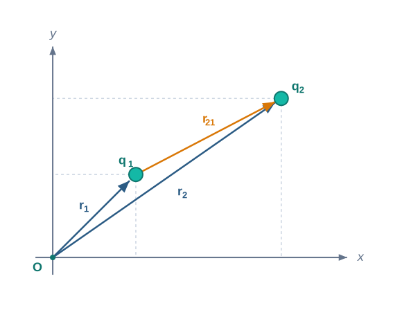
Fig. 1.8(a) – Vector notation for the force between two point charges.
The vector pointing from charge 1 to charge 2 is
\[\vec{r}_{21} = \vec{r}_2 - \vec{r}_1\]
and the vector pointing from charge 2 to charge 1 is
\[\vec{r}_{12} = \vec{r}_1 - \vec{r}*2 = -\vec{r}*{21}\]
The magnitudes of these vectors are written \(r_{21}\) and \(r_{12}\), and clearly \(r_{12} = r_{21}\) (the distance between the two charges is the same either way). To specify direction, we use unit vectors — vectors of length 1 that point along a given direction:
\[\hat{r}*{21} = \frac{\vec{r}*{21}}{r_{21}}, \qquad \hat{r}*{12} = \frac{\vec{r}*{12}}{r_{12}}, \qquad \hat{r}*{21} = -\hat{r}*{12}\]
With these, Coulomb’s force law for two point charges \(q_1\) and \(q_2\) located at \(\vec{r}_1\) and \(\vec{r}_2\) is written as
\[\vec{F}*{21} = \frac{1}{4\pi\varepsilon_0}\frac{q_1 q_2}{r*{21}^2},\hat{r}_{21} \tag{1.3}\]
Here \(\vec{F}*{21}\) is the force on \(q_2\) due to \(q_1\), and \(\hat{r}*{21}\) is the unit vector pointing from \(q_1\) toward \(q_2\).
What the vector form tells us
A few remarks make clear why the vector form is so useful.
First, Eq. (1.3) works for any signs of \(q_1\) and \(q_2\) — we do not need separate formulas for attraction and repulsion. If the two charges have the same sign (both positive or both negative), the product \(q_1 q_2\) is positive, so \(\vec{F}*{21}\) points along \(\hat{r}*{21}\) — away from \(q_1\) — which correctly means repulsion. If the charges have opposite signs, \(q_1 q_2\) is negative, so \(\vec{F}*{21}\) points along \(-\hat{r}*{21} = \hat{r}_{12}\) — toward \(q_1\) — which correctly means attraction. Fig. 1.8(b) shows both cases.
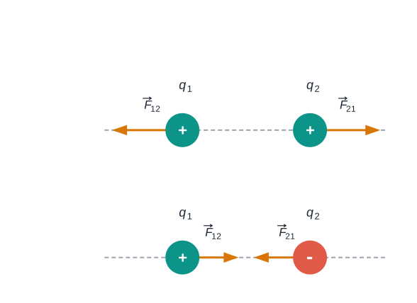
Fig. 1.8(b) – Force directions for like and unlike charges.
Second, the force on \(q_1\) due to \(q_2\) is obtained simply by swapping the labels 1 and 2:
\[\vec{F}*{12} = \frac{1}{4\pi\varepsilon_0}\frac{q_1 q_2}{r*{12}^2},\hat{r}*{12} = -\vec{F}*{21}\]
So the two forces are equal in magnitude and opposite in direction. This means Coulomb’s law is consistent with Newton’s third law — the two charges push or pull on each other with equal and opposite forces.
Third, Coulomb’s law as written in Eq. (1.3) gives the force between two charges in vacuum. If the charges are placed in some material medium, or the space between them contains matter, the situation becomes more complicated because of the charged constituents of the matter. That case will be taken up in the next chapter.
A charged metallic sphere A is hung from a nylon thread. Another charged metallic sphere B, held by an insulating handle, is brought close to A so that the distance between their centres is 10 cm, as in Fig. 1.9(a). The repulsion of A is noted. Spheres A and B are then touched by uncharged spheres C and D respectively, as in Fig. 1.9(b). After C and D are removed, B is brought closer to A so that the distance between their centres is now 5.0 cm, as in Fig. 1.9(c). What repulsion of A is expected on the basis of Coulomb’s law? Spheres A and C have identical sizes, and so do B and D. Ignore the sizes of A and B compared with the separation between their centres.
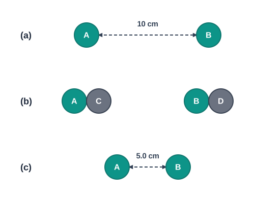
[Caption:] Fig. 1.9 – (a) Initial separation, (b) charge sharing, and (c) final separation. [/Caption:]
Each touch of an identical uncharged sphere halves the charge (by symmetry), and halving the distance strengthens the force — we track how these two effects combine.
Let the original charge on sphere A be \(q\) and that on B be \(q'\). At a separation \(r\) between their centres, the magnitude of the force on each is
\[F = \frac{1}{4\pi\varepsilon_0}\frac{qq'}{r^2}\]
neglecting the sizes of A and B compared with \(r\). When the identical uncharged sphere C touches A, the charge redistributes equally, so each carries \(q/2\). Similarly, after D touches B, each carries \(q'/2\). Now the separation between A and B is halved to \(r/2\), so the new force is
\[F' = \frac{1}{4\pi\varepsilon_0}\frac{(q/2)(q'/2)}{(r/2)^2} = \frac{1}{4\pi\varepsilon_0}\frac{qq'}{r^2} = F\]
Thus the electrostatic force on A due to B remains unchanged. The halving of each charge (which would reduce the force to one-fourth) is exactly cancelled by the halving of the distance (which would increase the force fourfold).
1.6 Forces between Multiple Charges
Coulomb’s law tells us the force between just two point charges. But in most real situations, a charge is surrounded not by one other charge but by several. Suppose we have a system of \(n\) stationary charges \(q_1, q_2, q_3, \ldots, q_n\) in vacuum, and we want the force on \(q_1\) due to all the others. Coulomb’s law by itself does not immediately answer this — it only handles pairs.
To go further, we need to know how the individual pair-forces combine. Recall from mechanics that ordinary forces add according to the parallelogram law of vector addition. The natural question is: do electrostatic forces add in the same way?
The principle of superposition
Experiment gives a clear answer. The force on any one charge due to a number of other charges is simply the vector sum of all the separate forces acting on it — the force from each other charge taken one at a time, as if the others were not there. Crucially, each individual pair-force is unaffected by the presence of the other charges. This experimentally established fact is called the principle of superposition.
Force from two charges
Let us start with three charges \(q_1\), \(q_2\), and \(q_3\), as shown in Fig. 1.10(a). To find the force on \(q_1\), we work out the force from each of the other two separately, then add them as vectors.
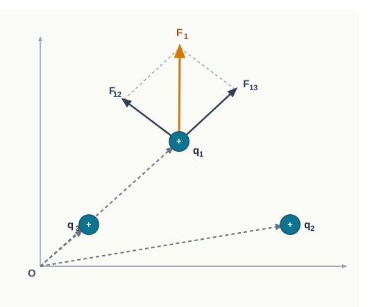
Fig. 1.10(a) – Superposition of electric forces from two point charges.
The force on \(q_1\) due to \(q_2\), written \(\vec{F}_{12}\), is given by Coulomb’s law exactly as before — the presence of \(q_3\) makes no difference to it:
\[\vec{F}*{12} = \frac{1}{4\pi\varepsilon_0}\frac{q_1 q_2}{r*{12}^2},\hat{r}_{12}\]
where \(r_{12}\) is the distance between \(q_1\) and \(q_2\), and \(\hat{r}_{12}\) is the unit vector pointing from \(q_2\) toward \(q_1\).
In the same way, the force on \(q_1\) due to \(q_3\), written \(\vec{F}_{13}\), is
\[\vec{F}*{13} = \frac{1}{4\pi\varepsilon_0}\frac{q_1 q_3}{r*{13}^2},\hat{r}_{13}\]
which is again just the Coulomb force on \(q_1\) due to \(q_3\), unaffected by the presence of \(q_2\).
The total force \(\vec{F}_1\) on \(q_1\) due to both \(q_2\) and \(q_3\) is the vector sum of these two forces:
\[\vec{F}*1 = \vec{F}*{12} + \vec{F}*{13} = \frac{1}{4\pi\varepsilon_0}\frac{q_1 q_2}{r*{12}^2},\hat{r}*{12} + \frac{1}{4\pi\varepsilon_0}\frac{q_1 q_3}{r*{13}^2},\hat{r}_{13} \tag{1.4}\]
Generalising to many charges
This idea extends directly to any number of charges, as suggested in Fig. 1.10(b). The principle of superposition assures us that the force on \(q_1\) due to \(q_2\) is exactly the Coulomb force between them, no matter how many other charges \(q_3, q_4, \ldots, q_n\) are also present.
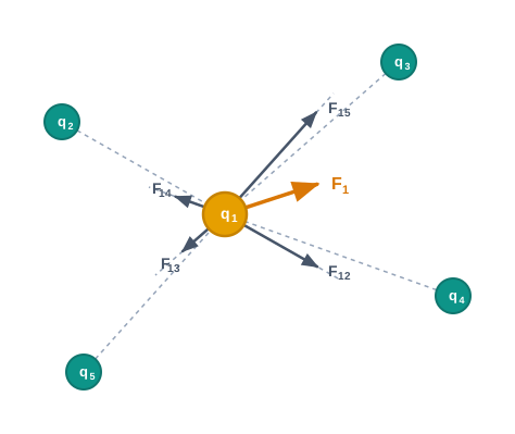
Fig. 1.10(b) – Superposition of electric forces from multiple point charges.
So the total force \(\vec{F}*1\) on \(q_1\) due to all the other charges is the vector sum of the individual forces \(\vec{F}*{12}, \vec{F}*{13}, \ldots, \vec{F}*{1n}\):
\[\vec{F}*1 = \vec{F}*{12} + \vec{F}*{13} + \cdots + \vec{F}*{1n} = \frac{1}{4\pi\varepsilon_0}\left[\frac{q_1 q_2}{r_{12}^2},\hat{r}*{12} + \frac{q_1 q_3}{r*{13}^2},\hat{r}*{13} + \cdots + \frac{q_1 q_n}{r*{1n}^2},\hat{r}_{1n}\right]\]
This can be written compactly using summation notation:
\[\vec{F}*1 = \frac{q_1}{4\pi\varepsilon_0}\sum*{i=2}^{n}\frac{q_i}{r_{1i}^2},\hat{r}_{1i} \tag{1.5}\]
Here the sum runs over all the other charges \(i = 2, 3, \ldots, n\); \(r_{1i}\) is the distance between \(q_1\) and the \(i\)-th charge, and \(\hat{r}_{1i}\) is the unit vector pointing from the \(i\)-th charge toward \(q_1\). As always, this vector sum is carried out using the parallelogram law of vector addition.
This simple-looking result is remarkably powerful. In fact, all of electrostatics is basically a consequence of just two ideas: Coulomb’s law and the superposition principle. Everything else is built on top of these two.
Three charges \(q_1\), \(q_2\), \(q_3\), each equal to \(q\), are placed at the vertices of an equilateral triangle of side \(l\). What is the force on a charge \(Q\) (with the same sign as \(q\)) placed at the centroid of the triangle, as shown in Fig. 1.11?
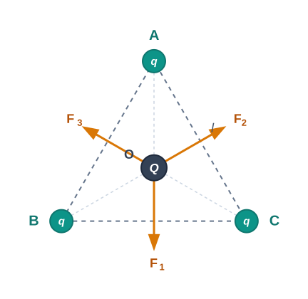
[Caption:] Fig. 1.11 – Forces on a charge at the centroid of an equilateral triangle. [/Caption:]
The key is symmetry: the three vertex charges are identical and equally distant from the centre, so their forces on \(Q\) should balance out. We verify this by computing each force and adding them.
In the equilateral triangle ABC of side \(l\), drop a perpendicular AD to the side BC. Then
\[\text{AD} = \text{AC}\cos 30^\circ = \frac{\sqrt{3}}{2}, l\]
The centroid O lies two-thirds of the way from A along this perpendicular, so the distance AO is
\[\text{AO} = \frac{2}{3},\text{AD} = \frac{1}{\sqrt{3}}, l\]
By symmetry, AO = BO = CO, so all three charges are the same distance \(\dfrac{l}{\sqrt{3}}\) from \(Q\). Using Coulomb’s law, each force has magnitude \(\dfrac{1}{4\pi\varepsilon_0}\dfrac{3Qq}{l^2}\) (since \(r^2 = l^2/3\)):
Force \(\vec{F}_1\) on \(Q\) due to \(q\) at A \(= \dfrac{1}{4\pi\varepsilon_0}\dfrac{3Qq}{l^2}\) directed along AO
Force \(\vec{F}_2\) on \(Q\) due to \(q\) at B \(= \dfrac{1}{4\pi\varepsilon_0}\dfrac{3Qq}{l^2}\) directed along BO
Force \(\vec{F}_3\) on \(Q\) due to \(q\) at C \(= \dfrac{1}{4\pi\varepsilon_0}\dfrac{3Qq}{l^2}\) directed along CO
By the parallelogram law, the resultant of \(\vec{F}_2\) and \(\vec{F}_3\) has magnitude \(\dfrac{1}{4\pi\varepsilon_0}\dfrac{3Qq}{l^2}\) directed along OA — that is, exactly opposite to \(\vec{F}_1\). Therefore the total force on \(Q\) is
\[\vec{F} = \frac{1}{4\pi\varepsilon_0}\frac{3Qq}{l^2}(\hat{r} - \hat{r}) = 0\]
where \(\hat{r}\) is the unit vector along OA. The net force on \(Q\) is zero.
There is also an elegant symmetry argument for this. Suppose the resultant force were not zero but pointed in some definite direction. Now imagine rotating the whole system by \(60^\circ\) about the centre O. The arrangement of charges looks exactly the same as before, so the force must be the same — yet it would now point in a different direction. The only way a force can stay the same while pointing in a new direction is if it is zero. Hence the net force must vanish.
Consider charges \(q\), \(q\), and \(-q\) placed at the vertices of an equilateral triangle, as shown in Fig. 1.12. What is the force on each charge?
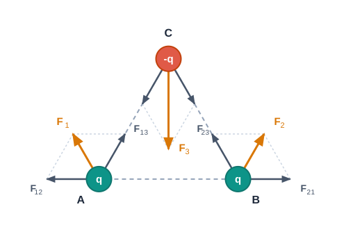
[Caption:] Fig. 1.12 – Forces on charges at the vertices of an equilateral triangle. [/Caption:]
Here the charges are not all alike, so the forces will not cancel. We use superposition at each vertex, adding the two pair-forces as vectors.
The forces acting on charge \(q\) at A come from \(q\) at B and from \(-q\) at C. These are \(\vec{F}*{12}\) directed along BA (repulsion) and \(\vec{F}*{13}\) directed along AC (attraction), as shown in Fig. 1.12. By the parallelogram law, the total force \(\vec{F}_1\) on the charge at A is
\[\vec{F}_1 = F,\hat{r}_1\]
where \(\hat{r}_1\) is a unit vector along BC. The magnitude of the attraction or repulsion for each pair of charges is the same:
\[F = \frac{q^2}{4\pi\varepsilon_0, l^2}\]
Similarly, the total force \(\vec{F}_2\) on the charge \(q\) at B is
\[\vec{F}_2 = F,\hat{r}_2\]
where \(\hat{r}_2\) is a unit vector along AC.
Finally, the total force on the charge \(-q\) at C is
\[\vec{F}_3 = \sqrt{3}, F,\hat{n}\]
where \(\hat{n}\) is the unit vector along the direction bisecting the angle BCA. Note that the forces on the two positive charges each have magnitude \(F\), while the force on the negative charge has magnitude \(\sqrt{3},F\).
An interesting check: the sum of the forces on all three charges is zero,
\[\vec{F}_1 + \vec{F}_2 + \vec{F}_3 = 0\]
This is not surprising. It follows directly from the fact that Coulomb’s law obeys Newton’s third law — every internal force between a pair of charges is matched by an equal and opposite force, so all the internal forces cancel when summed over the whole system. (Working this out in full is left as an exercise.)
1.7 Electric Field
We now come to one of the most important ideas in all of physics: the electric field. To see why it is needed, let us ask a simple but deep question.
Consider a point charge \(Q\) placed at the origin O. If we put another point charge \(q\) at a point P, at a distance \(r\) from O, then \(Q\) exerts a force on \(q\) as given by Coulomb’s law. That is clear enough. But now suppose we remove \(q\). What is left behind at P? Is there simply nothing there?
If there is nothing at P, then how does a force suddenly appear the moment we place a charge \(q\) at that point? The two charges never touch — so how does one “know” the other is there? This puzzle troubled early scientists, and to resolve it they introduced the concept of a field.
The idea of a field
The answer is this: the charge \(Q\) produces an electric field everywhere in the space around it, whether or not any other charge is present. This field is a real physical condition of the space. When another charge \(q\) is brought to a point P, the field already there acts on \(q\) and produces the force we observe.
The electric field produced by a charge \(Q\) at a point with position vector \(\vec{r}\) is defined as
\[\vec{E}(\vec{r}) = \frac{1}{4\pi\varepsilon_0}\frac{Q}{r^2},\hat{r} \tag{1.6}\]
where \(Q\) is the source charge in coulombs (C), \(r\) is the distance from the charge to the point in metres (m), and \(\hat{r} = \vec{r}/r\) is the unit vector pointing from the charge toward the point. The electric field \(\vec{E}\) is measured in newtons per coulomb (N/C).
Equation (1.6) gives the value of the electric field for every position vector \(\vec{r}\) — that is, at every point in space. The very word “field” signifies how some quantity (which may be a scalar or a vector) is spread out over space and varies from point to point. The effect of the charge \(Q\) is now built into the existence of this field.
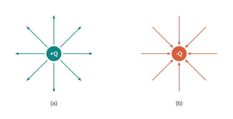
Fig. 1.13 – Electric field lines of (a) a positive charge and (b) a negative charge.
Force in terms of the field
Once we know the field, we can find the force on any charge placed in it. The force \(\vec{F}\) that the charge \(Q\) exerts on a charge \(q\) is
\[\vec{F} = \frac{1}{4\pi\varepsilon_0}\frac{Qq}{r^2},\hat{r} \tag{1.7}\]
Comparing Eq. (1.6) and Eq. (1.7), we see the force is simply the charge \(q\) multiplied by the field \(\vec{E}\) at its location. Writing the position of \(q\) as \(\vec{r}\),
\[\vec{F}(\vec{r}) = q,\vec{E}(\vec{r}) \tag{1.8}\]
This compact and powerful relation says the force on a charge equals that charge times the electric field where it sits. It also defines the SI unit of electric field: from \(\vec{E} = \vec{F}/q\), the unit is newton per coulomb (N/C). (An alternative unit, volt per metre, V/m, will appear in the next chapter.)
Note that by Newton’s third law, the charge \(q\) also exerts an equal and opposite force on \(Q\). We can look at the electrostatic force between \(Q\) and \(q\) in a symmetric way: as an interaction between \(q\) and the field of \(Q\), or equally as an interaction between \(Q\) and the field of \(q\).
Some important remarks about the electric field
(i) Field as force on a unit test charge. From Eq. (1.8), if \(q = 1\), the electric field is numerically equal to the force on it. So the electric field due to a charge \(Q\) at a point can be defined as the force that a unit positive charge would experience if placed at that point.
The charge \(Q\) that produces the field is called the source charge, and the small charge \(q\) used to test the field is called the test charge.
There is a subtlety here. The source charge \(Q\) must stay at its original position. But if we bring a test charge \(q\) nearby, then \(Q\) will itself feel a force from \(q\) and tend to move. To avoid disturbing \(Q\), we make the test charge \(q\) negligibly small. Then the force \(\vec{F}\) on it is also negligibly small, but the ratio \(\vec{F}/q\) stays finite and gives the field:
\[\vec{E} = \lim_{q\to 0}\left(\frac{\vec{F}}{q}\right) \tag{1.9}\]
In practice, the problem of keeping the source charge fixed is handled by holding it in place with other forces. For example, when we later study the field of a charged sheet (Section 1.14), the charges on the sheet are held in place by the forces of the material making up the sheet.
(ii) The field is independent of the test charge. Although we define \(\vec{E}\) using a test charge \(q\), the field itself does not depend on \(q\). This is because the force \(\vec{F}\) is proportional to \(q\), so the ratio \(\vec{F}/q\) cancels out any dependence on \(q\). The field \(\vec{E}\) due to \(Q\) depends only on the position \(\vec{r}\) — it exists at every point in three-dimensional space, and takes a different value at each point.
(iii) Direction of the field. For a positive source charge, the electric field points radially outward, away from the charge. For a negative source charge, the field at every point points radially inward, toward the charge. This is exactly what Fig. 1.13 shows.
(iv) Spherical symmetry. Since the magnitude of the force depends only on the distance \(r\) from the source charge, the magnitude of \(\vec{E}\) also depends only on \(r\). So at all points the same distance from \(Q\), the field has the same magnitude. In other words, the field of a point charge has the same magnitude everywhere on a sphere centred on the charge — it has spherical symmetry.
1.7.1 Electric field due to a system of charges
Just as a single charge sets up a field, so does a whole collection of charges. Consider a system of charges \(q_1, q_2, \ldots, q_n\) with position vectors \(\vec{r}_1, \vec{r}_2, \ldots, \vec{r}_n\) relative to an origin O.
The field of the system at a point P is defined just as before: it is the force experienced by a unit test charge placed at P, without disturbing the original positions of the charges. To find it, we combine Coulomb’s law with the superposition principle.
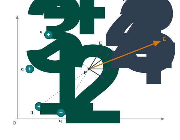
Fig. 1.14 – Superposition of electric fields from a system of charges.
The field \(\vec{E}_1\) at P due to \(q_1\) (located at \(\vec{r}_1\)) is
\[\vec{E}*1 = \frac{1}{4\pi\varepsilon_0}\frac{q_1}{r*{1P}^2},\hat{r}_{1P}\]
where \(\hat{r}*{1P}\) is the unit vector pointing from \(q_1\) toward P, and \(r*{1P}\) is the distance between \(q_1\) and P.
In the same way, the field \(\vec{E}_2\) at P due to \(q_2\) is
\[\vec{E}*2 = \frac{1}{4\pi\varepsilon_0}\frac{q_2}{r*{2P}^2},\hat{r}_{2P}\]
where \(r_{2P}\) is the distance from \(q_2\) to P. Similar expressions hold for the fields \(\vec{E}_3, \vec{E}_4, \ldots, \vec{E}_n\) due to the remaining charges.
By the superposition principle, the total electric field \(\vec{E}\) at P due to the whole system is the vector sum of the individual fields:
\[\vec{E}(\vec{r}) = \vec{E}_1(\vec{r}) + \vec{E}_2(\vec{r}) + \cdots + \vec{E}_n(\vec{r})\]
\[= \frac{1}{4\pi\varepsilon_0}\frac{q_1}{r_{1P}^2},\hat{r}*{1P} + \frac{1}{4\pi\varepsilon_0}\frac{q_2}{r*{2P}^2},\hat{r}*{2P} + \cdots + \frac{1}{4\pi\varepsilon_0}\frac{q_n}{r*{nP}^2},\hat{r}_{nP}\]
which can be written compactly as
\[\vec{E}(\vec{r}) = \frac{1}{4\pi\varepsilon_0}\sum_{i=1}^{n}\frac{q_i}{r_{iP}^2},\hat{r}_{iP} \tag{1.10}\]
Here the sum runs over all \(n\) charges, \(r_{iP}\) is the distance from the \(i\)-th charge to P, and \(\hat{r}_{iP}\) is the unit vector from the \(i\)-th charge toward P. The electric field \(\vec{E}\) is a vector quantity that varies from one point to another, and it is completely determined by the positions and sizes of the source charges.
1.7.2 Physical significance of electric field
You may reasonably wonder why we bother introducing the electric field at all. After all, for any system of charges, the thing we can actually measure is the force on a charge — and that we can already find directly using Coulomb’s law and superposition, as in Eq. (1.5). So why introduce this intermediate quantity called the field?
For electrostatics — charges at rest — the honest answer is that the field is convenient but not strictly necessary. It is an elegant way of describing the electrical environment around a system of charges. The field at a point tells you the force a unit positive test charge would feel there, without your having to redo the whole calculation each time. Importantly, the field is a property of the source charges alone; it does not depend on the test charge you use to probe it. In general, the term “field” in physics means a quantity defined at every point in space that may vary from point to point. Since force is a vector, the electric field is a vector field.
The deeper significance
The true physical importance of the field appears only when we go beyond static charges and consider time-dependent situations. Suppose two distant charges \(q_1\) and \(q_2\) are in accelerated motion. The fastest that any signal or information can travel from one point to another is \(c\), the speed of light. So if \(q_1\) suddenly moves, the effect on \(q_2\) cannot happen instantly — there must be a time delay between the cause (the motion of \(q_1\)) and the effect (the change in force on \(q_2\)).
This is exactly where the field concept becomes essential. The picture is this: the accelerated motion of \(q_1\) produces electromagnetic waves, which travel outward at the speed \(c\), reach \(q_2\) after some delay, and then exert a force on it. The field neatly accounts for the time delay that Coulomb’s law alone cannot handle.
So even though electric and magnetic fields can be detected only through their effects (forces) on charges, they are regarded as genuine physical entities in their own right, not mere mathematical constructs. They have an independent dynamics — they evolve according to their own laws — and they can transport energy through space.
An electron falls through a distance of \(1.5\) cm in a uniform electric field of magnitude \(2.0 \times 10^{4}\) N C\(^{-1}\), as in Fig. 1.15(a). The direction of the field is then reversed, keeping its magnitude the same, and a proton falls through the same distance, as in Fig. 1.15(b). Compute the time of fall in each case, and contrast the situation with ‘free fall under gravity’.
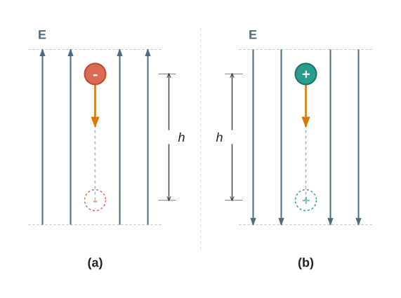
[Caption:] Fig. 1.15 – Acceleration of (a) an electron and (b) a proton in a uniform electric field. [/Caption:]
In each case the electric force plays the role of gravity, giving the particle a constant acceleration. We use the same kinematics as free fall, but with acceleration \(eE/m\) instead of \(g\).
In Fig. 1.15(a), the field points upward, so the negatively charged electron feels a downward force of magnitude \(eE\), where \(E\) is the field magnitude. The acceleration of the electron is
\[a_e = \frac{eE}{m_e}\]
where \(m_e\) is the mass of the electron. Starting from rest, the time to fall a distance \(h\) is
\[t_e = \sqrt{\frac{2h}{a_e}} = \sqrt{\frac{2h, m_e}{eE}}\]
Substituting \(e = 1.6 \times 10^{-19}\) C, \(m_e = 9.11 \times 10^{-31}\) kg, \(E = 2.0 \times 10^{4}\) N C\(^{-1}\), and \(h = 1.5 \times 10^{-2}\) m gives
\[t_e = 2.9 \times 10^{-9} \ \text{s}\]
In Fig. 1.15(b), the field points downward, so the positively charged proton also feels a downward force of magnitude \(eE\). Its acceleration is
\[a_p = \frac{eE}{m_p}\]
where \(m_p = 1.67 \times 10^{-27}\) kg is the proton mass. The time of fall for the proton is
\[t_p = \sqrt{\frac{2h}{a_p}} = \sqrt{\frac{2h, m_p}{eE}} = 1.3 \times 10^{-7} \ \text{s}\]
The heavier proton takes a much longer time to fall the same distance. This is in sharp contrast to free fall under gravity, where the time of fall does not depend on the mass of the body.
Note that we ignored gravity in this problem. To check that this is justified, calculate the proton’s acceleration due to the electric field:
\[a_p = \frac{eE}{m_p} = \frac{(1.6 \times 10^{-19}\ \text{C})\times(2.0 \times 10^{4}\ \text{N C}^{-1})}{1.67 \times 10^{-27}\ \text{kg}} = 1.9 \times 10^{12} \ \text{m s}^{-2}\]
This is enormous compared with \(g = 9.8\ \text{m s}^{-2}\), and the electron’s acceleration is even larger. So the effect of gravity is completely negligible here.
Two point charges \(q_1\) and \(q_2\), of magnitude \(+10^{-8}\) C and \(-10^{-8}\) C respectively, are placed \(0.1\) m apart. Calculate the electric fields at points A, B, and C shown in Fig. 1.16.
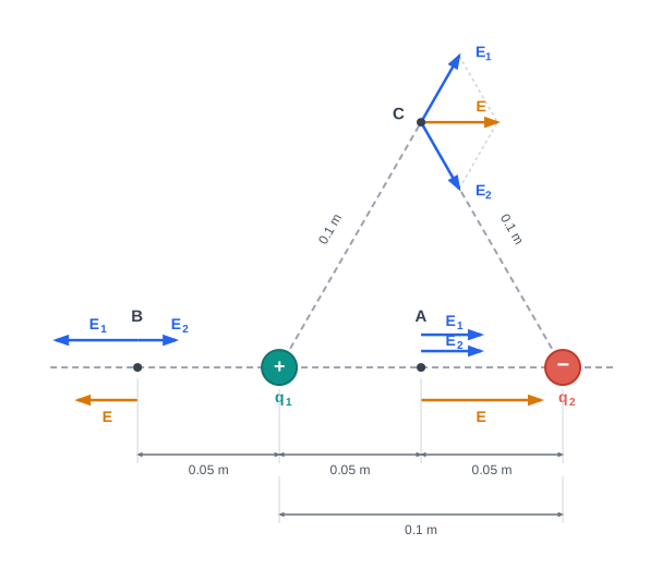
[Caption:] Fig. 1.16 – Electric field at points A, B, and C due to two point charges. [/Caption:]
We find the field due to each charge separately at each point, keeping track of direction, then add them as vectors.
The field \(\vec{E}_{1A}\) at A due to the positive charge \(q_1\) points toward the right, with magnitude
\[E_{1A} = \frac{(9 \times 10^{9}\ \text{Nm}^2\text{C}^{-2}) \times (10^{-8}\ \text{C})}{(0.05\ \text{m})^2} = 3.6 \times 10^{4} \ \text{N C}^{-1}\]
The field \(\vec{E}_{2A}\) at A due to the negative charge \(q_2\) also points toward the right (toward the negative charge) and has the same magnitude. So the total field at A is
\[E_A = E_{1A} + E_{2A} = 7.2 \times 10^{4} \ \text{N C}^{-1}\]
directed toward the right.
The field \(\vec{E}_{1B}\) at B due to \(q_1\) points toward the left, with magnitude
\[E_{1B} = \frac{(9 \times 10^{9}\ \text{Nm}^2\text{C}^{-2}) \times (10^{-8}\ \text{C})}{(0.05\ \text{m})^2} = 3.6 \times 10^{4} \ \text{N C}^{-1}\]
The field \(\vec{E}_{2B}\) at B due to \(q_2\) points toward the right, with magnitude
\[E_{2B} = \frac{(9 \times 10^{9}\ \text{Nm}^2\text{C}^{-2}) \times (10^{-8}\ \text{C})}{(0.15\ \text{m})^2} = 4 \times 10^{3} \ \text{N C}^{-1}\]
Since these point in opposite directions, the total field at B is
\[E_B = E_{1B} - E_{2B} = 3.2 \times 10^{4} \ \text{N C}^{-1}\]
directed toward the left.
At point C, the fields due to \(q_1\) and \(q_2\) have equal magnitude:
\[E_{1C} = E_{2C} = \frac{(9 \times 10^{9}\ \text{Nm}^2\text{C}^{-2}) \times (10^{-8}\ \text{C})}{(0.10\ \text{m})^2} = 9 \times 10^{3} \ \text{N C}^{-1}\]
The directions of these two fields are indicated in Fig. 1.16. Their components perpendicular to the line AB cancel, while the components along AB add. The resultant is
\[E_C = E_{1C}\cos\frac{\pi}{3} + E_{2C}\cos\frac{\pi}{3} = 9 \times 10^{3} \ \text{N C}^{-1}\]
pointing toward the right (parallel to AB).
1.8 Electric Field Lines
In the previous section we learned that the electric field is a vector quantity — it has both magnitude and direction at every point in space. Since it is a vector, we can represent it using arrows. But a field fills all of space, and drawing an arrow at every single point would quickly become a hopeless tangle. Electric field lines give us a cleaner, more intuitive way to picture the field.
From arrows to lines
Let us try to represent the field of a single point charge placed at the origin. At each point around the charge, we draw a small arrow pointing along the direction of the field, with a length proportional to the strength of the field there.
Because the magnitude of the field falls off as the square of the distance from the charge, the arrows get shorter and shorter as we move outward, while always pointing radially outward from a positive charge. This is shown in Fig. 1.17, where each arrow represents the field — that is, the force on a unit positive charge placed at the tail of that arrow.

Fig. 1.17 – Field of a point charge.
Now connect the arrows that point in the same direction into continuous curves. Each such curve is called a field line. For a point charge, we get many field lines all radiating outward from the charge.
Where did the strength information go?
You might worry that we have lost information. The length of each arrow told us the strength of the field — but once we join arrows into lines, the lengths are gone. Has the magnitude information disappeared?
No. The magnitude is now captured in a different way: by the density of the field lines — how closely packed they are. Near the charge, where the field is strong, the lines are crowded close together. Far from the charge, where the field is weak, the lines spread out and become well separated.
Why line density represents field strength
There is a beautiful reason why the density of field lines correctly represents the strength of the field. We draw the figure on a flat sheet of paper, in two dimensions, but we actually live in three dimensions. To measure the density of field lines properly, we should count the number of lines passing through a unit area held perpendicular to the lines.
Now think about a point charge. As we move away from it, the field decreases as the square of the distance (\(1/r^2\)). At the same time, the area of a surface enclosing the charge (like a sphere) increases as the square of the distance (\(r^2\)). These two effects exactly compensate. So the total number of field lines crossing any enclosing surface stays the same, no matter how far that surface is from the charge. The lines are neither created nor destroyed as we move outward — they just spread over a larger area.
This is why field lines carry information about both the direction and the strength of the field. Once a set of lines is drawn, their relative closeness at different points tells us the relative strength of the field: the lines crowd together where the field is strong and spread apart where it is weak. Fig. 1.18 shows such a set of lines, with a strong-field region and a weak-field region.
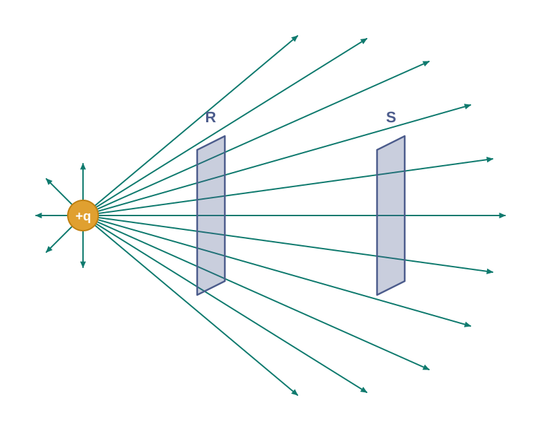
Fig. 1.18 – Field line density and field strength.
Imagine two equal, small area elements placed at points R and S, each held perpendicular (normal) to the field lines there. The number of field lines cutting through each element is proportional to the strength of the field at that point. In Fig. 1.18, more lines pass through the element at R than at S, showing that the field at R is stronger than at S.
Solid angle and the \(1/r^2\) law
We can make this precise using the idea of a solid angle, which is simply the three-dimensional version of an ordinary angle. First recall the two-dimensional case: if a small transverse line element \(\Delta l\) is placed at a distance \(r\) from a point O, the plane angle it subtends at O is approximately
\[\Delta\theta = \frac{\Delta l}{r}\]
In three dimensions, a small flat area \(\Delta S\) placed perpendicular to the line of sight at a distance \(r\) subtends a solid angle
\[\Delta\Omega = \frac{\Delta S}{r^2}\]
The key fact is that within a given solid angle, the number of radial field lines is always the same. In Fig. 1.18, consider two points \(P_1\) and \(P_2\) at distances \(r_1\) and \(r_2\) from the charge. The area needed to subtend the same solid angle \(\Delta\Omega\) is \(r_1^2,\Delta\Omega\) at \(P_1\) and \(r_2^2,\Delta\Omega\) at \(P_2\). The same number of lines, say \(n\), cuts through both of these areas.
So the number of lines cutting unit area is \(\dfrac{n}{r_1^2,\Delta\Omega}\) at \(P_1\) and \(\dfrac{n}{r_2^2,\Delta\Omega}\) at \(P_2\). Since \(n\) and \(\Delta\Omega\) are the same in both cases, the density of lines — and hence the field strength — clearly varies as \(1/r^2\). The field-line picture and Coulomb’s inverse-square law fit together perfectly.
Definition of a field line
We can now state clearly what a field line is. An electric field line is a curve drawn so that the tangent to it at every point gives the direction of the net electric field at that point. An arrow on the curve is needed to show which of the two possible tangent directions the field actually points. A field line is a space curve — a curve in three dimensions.
Field lines of some charge arrangements
Fig. 1.19 shows the field lines around some simple charge arrangements. Remember that although the figure is drawn in a plane, the lines actually exist in three-dimensional space.
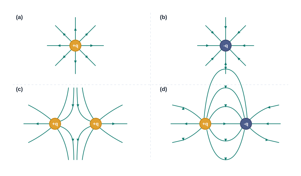
Fig. 1.19 – Field lines for simple charge configurations.
The field lines of a single positive charge point radially outward, while those of a single negative charge point radially inward. The lines around two positive charges \((q, q)\) curve away from each other, giving a vivid picture of their mutual repulsion. The lines around two equal and opposite charges \((q, -q)\) — an arrangement called a dipole — run from the positive to the negative charge, clearly showing the mutual attraction between them.
Properties of electric field lines
Field lines obey some important general rules:
Field lines start from positive charges and end on negative charges. If there is only a single charge, the lines may start or end at infinity.
In a region with no charge, electric field lines are continuous curves without any breaks.
Two field lines can never cross each other. If they did, then at the crossing point the field would have two different directions at once — which is impossible, since the field has a single, definite direction at every point.
Electrostatic field lines never form closed loops. This follows from the conservative nature of the electrostatic field, which you will study in Chapter 2.
1.9 Electric Flux
The field-line picture gives us a natural way to measure how much electric field passes through a given area. This quantity is called electric flux, and it will be the key to the powerful Gauss’s law we meet later. To build the idea, it helps to start with a familiar picture from the flow of a liquid.
An analogy: the flow of a liquid
Imagine a liquid flowing with velocity \(\vec{v}\) through a small flat surface of area \(\text{d}S\), held so that its surface is perpendicular (normal) to the flow. The rate at which liquid crosses the surface — the volume passing through per unit time — is \(v,\text{d}S\). This is called the flux of the liquid across the surface.
Now suppose the surface is not held perpendicular to the flow, but tilted so that its normal makes an angle \(\theta\) with the direction of flow \(\vec{v}\). Then only the projected area, \(\text{d}S\cos\theta\), faces the flow directly, and the flux across the surface is \(\vec{v}\cdot\hat{n},\text{d}S\).
For the electric field, we define an analogous quantity and call it the electric flux. There is one important difference to keep in mind: in the electric case, nothing physically flows. Unlike the liquid, there is no observable substance streaming across the surface. The “flux” here is just a measure of how much field passes through the area.
Counting field lines through an area
We saw earlier that the number of field lines crossing a unit area held normal to the field measures the strength of the field. So if we place a small flat area element \(\Delta S\) perpendicular to the field \(\vec{E}\) at a point, the number of field lines crossing it is proportional to \(E,\Delta S\).
Now tilt this area element by an angle \(\theta\), as shown in Fig. 1.20. Clearly, fewer field lines now cross it. The part of the area that effectively faces the field is its projection normal to \(\vec{E}\), which is \(\Delta S\cos\theta\). So the number of field lines crossing the tilted element is proportional to \(E,\Delta S\cos\theta\). When \(\theta = 90^\circ\), the field lines run parallel to the area element and do not cross it at all.
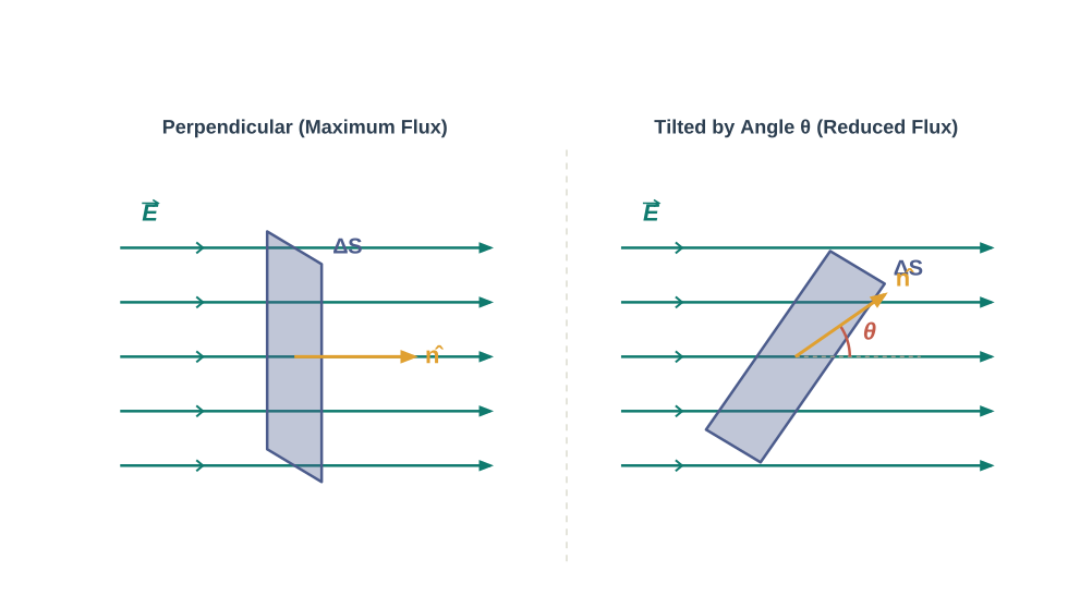
Fig. 1.20 – Area element in a uniform field.
Area as a vector
This example shows that the orientation of an area element — not just its size — matters. Think of holding a ring in a flowing stream: the amount of water passing through the ring depends on how you hold it. Held facing the flow, the maximum water passes through; held at an angle, less does. This tells us that an area element should be treated as a vector, with both a magnitude and a direction.
How do we assign a direction to a flat area? The normal to the plane — the line perpendicular to it — fixes the orientation of the surface. So the direction of a planar area vector is taken along its normal.
For a curved surface, we imagine dividing it into a large number of very small area elements. Each tiny element is nearly flat, so it can be treated as planar and assigned its own area vector, just as before.
Which way does the normal point?
There is one ambiguity to settle. A normal to a surface can point in either of two opposite directions — which one do we choose? For a closed surface (one that fully encloses a volume, like a balloon), there is a simple, universal convention: the area vector of every element points along the outward normal, away from the enclosed volume. This convention is shown in Fig. 1.21.
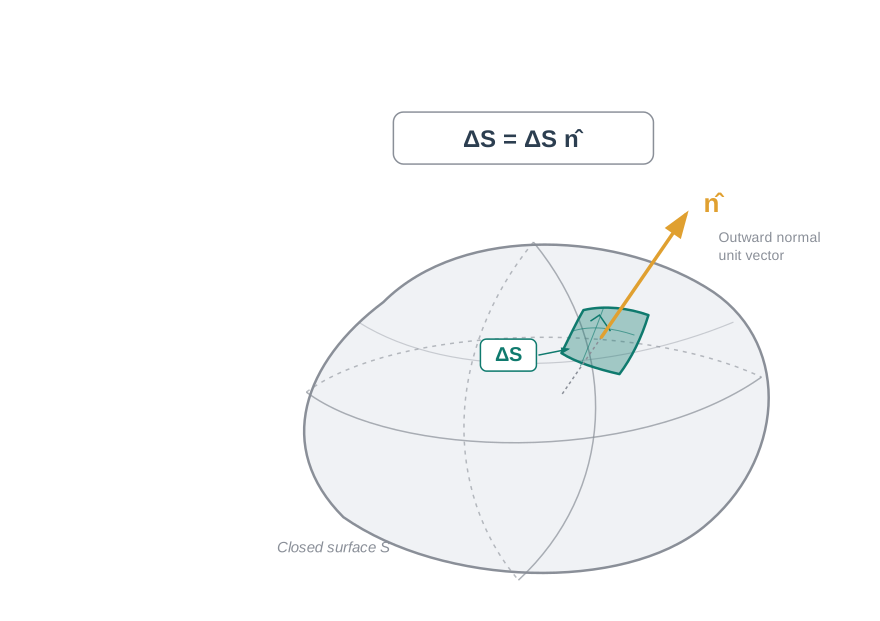
Fig. 1.21 – Outward normal vector convention.
So the area element vector at a point on a closed surface is written
\[\Delta\vec{S} = \Delta S,\hat{n}\]
where \(\Delta S\) is the magnitude of the area element and \(\hat{n}\) is the unit vector along the outward normal at that point.
Definition of electric flux
We can now define electric flux precisely. The electric flux \(\Delta\phi\) through a small area element \(\Delta\vec{S}\) is
\[\Delta\phi = \vec{E}\cdot\Delta\vec{S} = E,\Delta S\cos\theta \tag{1.11}\]
which, as we saw, is proportional to the number of field lines cutting through the area element. Here \(\theta\) is the angle between the field \(\vec{E}\) and the area vector \(\Delta\vec{S}\). For a closed surface, using the outward-normal convention, \(\theta\) is the angle between \(\vec{E}\) and the outward normal to the element.
We can read the expression \(E,\Delta S\cos\theta\) in two equivalent ways. Grouping it as \(E,(\Delta S\cos\theta)\), it is the field times the projection of the area normal to the field. Grouping it as \((E\cos\theta),\Delta S = E_\perp,\Delta S\), it is the component of the field along the normal, times the area of the element. Both readings give the same flux.
The SI unit of electric flux is newton coulomb\(^{-1}\) metre\(^2\) (N C\(^{-1}\) m\(^2\)).
Flux through a whole surface
The basic definition in Eq. (1.11) can be used, in principle, to find the total flux through any surface. We simply divide the surface into many small area elements, work out the flux \(\vec{E}\cdot\Delta\vec{S}\) through each one, and add them all up. The total flux \(\phi\) through a surface \(S\) is then
\[\phi \simeq \sum \vec{E}\cdot\Delta\vec{S} \tag{1.12}\]
The approximation sign appears because we have treated the field \(\vec{E}\) as constant over each small area element, which is only approximately true. The result becomes mathematically exact when we let the area elements shrink to zero (\(\Delta S \to 0\)); then the sum in Eq. (1.12) becomes an integral over the surface.
1.10 Electric Dipole
We have so far looked at single charges and simple systems of charges. We now study a very special and important arrangement called an electric dipole. Dipoles are important because many molecules behave like tiny dipoles, and because the dipole is the simplest charge arrangement whose total charge is zero yet whose field is not zero.
An electric dipole is a pair of equal and opposite point charges, \(+q\) and \(-q\), separated by a distance \(2a\). The line joining the two charges defines a direction in space. By convention, this direction is taken from \(-q\) to \(q\) — that is the direction of the dipole. The point exactly halfway between the two charges is called the centre of the dipole.
Why the dipole field is not zero
The total charge of a dipole is obviously zero, since \(+q\) and \(-q\) add to nothing. But this does not mean its electric field is zero. The two charges sit at slightly different places, so their fields at any point are not quite equal and opposite, and they do not perfectly cancel.
At distances much larger than the separation between the charges (\(r \gg 2a\)), the two fields very nearly cancel — but not completely. The small leftover field is the dipole field. Because of this near-cancellation, the field of a dipole falls off faster with distance than the field of a single charge: it decreases faster than \(1/r^2\). We will now confirm these qualitative ideas by direct calculation.
1.10.1 The field of an electric dipole
The field of the pair of charges \((-q\) and \(q)\) at any point can be found using Coulomb’s law and the superposition principle. The results are especially simple in two cases: when the point lies on the dipole axis, and when it lies in the equatorial plane — the plane perpendicular to the dipole axis passing through its centre. In general, the field at a point P is found by adding the field \(\vec{E}*{-q}\) due to \(-q\) and the field \(\vec{E}*{+q}\) due to \(+q\) by the parallelogram law.
(i) For points on the axis
Let the point P lie at a distance \(r\) from the centre of the dipole, on the side of the charge \(q\), as in Fig. 1.22(a). The charge \(-q\) is then at distance \((r+a)\) from P, and \(+q\) is at distance \((r-a)\) from P.
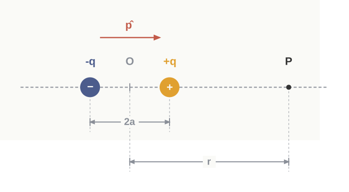
Fig. 1.22(a) – Dipole field on the axis.
The field at P due to \(-q\) points back toward \(-q\) (opposite to \(\hat{p}\)):
\[\vec{E}_{-q} = -\frac{q}{4\pi\varepsilon_0(r+a)^2},\hat{p} \tag{1.13a}\]
where \(\hat{p}\) is the unit vector along the dipole axis, from \(-q\) to \(q\). The field at P due to \(+q\) points away from \(+q\) (along \(\hat{p}\)):
\[\vec{E}_{+q} = \frac{q}{4\pi\varepsilon_0(r-a)^2},\hat{p} \tag{1.13b}\]
Adding these gives the total field at P:
\[\vec{E} = \vec{E}*{+q} + \vec{E}*{-q} = \frac{q}{4\pi\varepsilon_0}\left[\frac{1}{(r-a)^2} - \frac{1}{(r+a)^2}\right]\hat{p}\]
To simplify the bracket, we bring the two fractions to a common denominator. The numerator becomes \((r+a)^2 - (r-a)^2 = 4ar\), and the denominator becomes \((r^2 - a^2)^2\). So
\[\vec{E} = \frac{q}{4\pi\varepsilon_0}\frac{4ar}{(r^2-a^2)^2},\hat{p} \tag{1.14}\]
For points far from the dipole, \(r \gg a\), we can neglect \(a^2\) compared with \(r^2\), so \((r^2 - a^2)^2 \approx r^4\). This gives
\[\vec{E} = \frac{4qa}{4\pi\varepsilon_0 r^3},\hat{p} \qquad (r \gg a) \tag{1.15}\]
(ii) For points on the equatorial plane
Now let P lie in the equatorial plane, at distance \(r\) from the centre. Here each charge is at the same distance \(\sqrt{r^2 + a^2}\) from P, so the fields due to \(+q\) and \(-q\) have equal magnitudes:
\[E_{+q} = \frac{q}{4\pi\varepsilon_0}\frac{1}{r^2+a^2} \tag{1.16a}\]
\[E_{-q} = \frac{q}{4\pi\varepsilon_0}\frac{1}{r^2+a^2} \tag{1.16b}\]
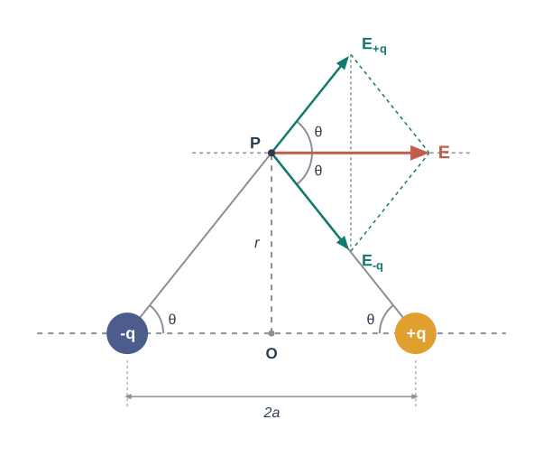
Fig. 1.22(b) – Dipole field on the equatorial plane.
The directions of \(\vec{E}*{+q}\) and \(\vec{E}*{-q}\) are shown in Fig. 1.22(b). When we add them, the components perpendicular to the dipole axis cancel, while the components along the axis add up. The resultant field points opposite to \(\hat{p}\). Each field contributes a component \(E\cos\theta\) along the axis, where \(\theta\) is the angle shown, with \(\cos\theta = \dfrac{a}{\sqrt{r^2+a^2}}\). Therefore
\[\vec{E} = -(E_{+q} + E_{-q})\cos\theta,\hat{p}\]
Substituting the magnitudes and \(\cos\theta\):
\[\vec{E} = -\frac{2qa}{4\pi\varepsilon_0(r^2+a^2)^{3/2}},\hat{p} \tag{1.17}\]
For large distances \(r \gg a\), we neglect \(a^2\) compared with \(r^2\), so \((r^2 + a^2)^{3/2} \approx r^3\), giving
\[\vec{E} = -\frac{2qa}{4\pi\varepsilon_0 r^3},\hat{p} \qquad (r \gg a) \tag{1.18}\]
The dipole moment
Compare the far-field results, Eq. (1.15) and Eq. (1.18). In both, the field at large distances does not depend on \(q\) and \(a\) separately — only on their product \(qa\). This suggests that we bundle them together into a single quantity, the dipole moment.
The dipole moment vector \(\vec{p}\) of an electric dipole is defined as
\[\vec{p} = q \times 2a,\hat{p} \tag{1.19}\]
That is, it is a vector whose magnitude is the charge \(q\) multiplied by the separation \(2a\) between the charges, and whose direction is along the line from \(-q\) to \(q\). The dipole moment is measured in coulomb metre (C m).
In terms of \(\vec{p}\), the far-field expressions take clean forms.
At a point on the dipole axis:
\[\vec{E} = \frac{2\vec{p}}{4\pi\varepsilon_0 r^3} \qquad (r \gg a) \tag{1.20}\]
At a point on the equatorial plane:
\[\vec{E} = -\frac{\vec{p}}{4\pi\varepsilon_0 r^3} \qquad (r \gg a) \tag{1.21}\]
Notice two important features. First, the dipole field falls off not as \(1/r^2\) (as for a single charge) but as \(1/r^3\) — it weakens much faster with distance. Second, the magnitude and direction of the dipole field depend not only on the distance \(r\) but also on the angle between the position vector \(\vec{r}\) and the dipole moment \(\vec{p}\).
The point dipole
We can imagine an idealised limit in which the size of the dipole \(2a\) shrinks toward zero, while the charge \(q\) grows toward infinity, in such a way that the product \(p = q \times 2a\) stays finite. Such an idealised dipole is called a point dipole. For a point dipole, the formulas in Eq. (1.20) and Eq. (1.21) are not just approximations — they are exact, true for any distance \(r\).
1.10.2 Physical significance of dipoles
Why do dipoles matter so much in nature? The answer lies in the structure of molecules.
In most molecules, the “centre” of all the positive charge and the “centre” of all the negative charge lie at the same point. For such molecules, the dipole moment is zero. Carbon dioxide (\(\text{CO}_2\)) and methane (\(\text{CH}_4\)) are examples of this type. However, even these molecules can develop a dipole moment when an external electric field is applied, because the field pulls the positive and negative charges slightly apart.
In some molecules, though, the centre of negative charge and the centre of positive charge do not coincide even without any applied field. These molecules have a permanent electric dipole moment, and are called polar molecules. Water (\(\text{H}_2\text{O}\)) is a well-known example. The behaviour of such polar materials, both in the presence and in the absence of an electric field, gives rise to many interesting properties and important applications.
Two charges \(\pm 10\ \mu\)C are placed \(5.0\) mm apart. Determine the electric field at (a) a point P on the axis of the dipole, \(15\) cm from its centre O on the side of the positive charge, as in Fig. 1.23(a), and (b) a point Q, \(15\) cm from O on a line through O perpendicular to the axis, as in Fig. 1.23(b).
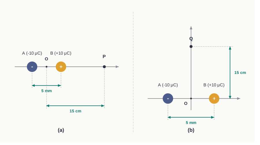
[Caption:] Fig. 1.23 – Electric field at points P and Q. [/Caption:]
In each part we first add the exact fields of the two charges, then check the answer against the far-field dipole formula, since the point is far compared with the tiny 5 mm separation.
(a) Point P on the axis. The half-separation is \(a = 2.5\) mm \(= 0.25\) cm, so \(+q\) (at B) is \((15 - 0.25)\) cm from P and \(-q\) (at A) is \((15 + 0.25)\) cm from P.
Field at P due to the \(+10\ \mu\)C charge:
\[\frac{10^{-5}\ \text{C}}{4\pi(8.854\times10^{-12}\ \text{C}^2\text{N}^{-1}\text{m}^{-2})} \times \frac{1}{(15-0.25)^2\times10^{-4}\ \text{m}^2} = 4.13 \times 10^{6}\ \text{N C}^{-1} \ \text{along BP}\]
Field at P due to the \(-10\ \mu\)C charge:
\[\frac{10^{-5}\ \text{C}}{4\pi(8.854\times10^{-12}\ \text{C}^2\text{N}^{-1}\text{m}^{-2})} \times \frac{1}{(15+0.25)^2\times10^{-4}\ \text{m}^2} = 3.86 \times 10^{6}\ \text{N C}^{-1} \ \text{along PA}\]
These point in opposite directions along the axis, so the resultant field at P is
\[E = 2.7 \times 10^{5}\ \text{N C}^{-1} \ \text{along BP}\]
Since the ratio OP/OB is quite large (\(= 60\)), we can also use the far-field axial formula and expect nearly the same answer. For a dipole of charges \(\pm q\) separated by \(2a\), the axial field at distance \(r\) is
\[E = \frac{2p}{4\pi\varepsilon_0 r^3} \qquad (r/a \gg 1)\]
where \(p = 2aq\) is the dipole moment, directed from \(-q\) to \(q\). Here
\[p = 10^{-5}\ \text{C} \times 5\times10^{-3}\ \text{m} = 5\times10^{-8}\ \text{C m}\]
so
\[E = \frac{2\times5\times10^{-8}\ \text{C m}}{4\pi(8.854\times10^{-12}\ \text{C}^2\text{N}^{-1}\text{m}^{-2})} \times \frac{1}{(15)^3\times10^{-6}\ \text{m}^3} = 2.6 \times 10^{5}\ \text{N C}^{-1}\]
directed along AB, close to the exact result found above.
(b) Point Q on the perpendicular line. Here each charge is the same distance from Q.
Field at Q due to \(+10\ \mu\)C at B:
\[\frac{10^{-5}\ \text{C}}{4\pi(8.854\times10^{-12}\ \text{C}^2\text{N}^{-1}\text{m}^{-2})} \times \frac{1}{[15^2+(0.25)^2]\times10^{-4}\ \text{m}^2} = 3.99 \times 10^{6}\ \text{N C}^{-1} \ \text{along BQ}\]
Field at Q due to \(-10\ \mu\)C at A:
\[\frac{10^{-5}\ \text{C}}{4\pi(8.854\times10^{-12}\ \text{C}^2\text{N}^{-1}\text{m}^{-2})} \times \frac{1}{[15^2+(0.25)^2]\times10^{-4}\ \text{m}^2} = 3.99 \times 10^{6}\ \text{N C}^{-1} \ \text{along QA}\]
The components of these two fields along OQ cancel, while their components parallel to BA add up. So the resultant field at Q is
\[2 \times \frac{0.25}{\sqrt{15^2+(0.25)^2}} \times 3.99\times10^{6}\ \text{N C}^{-1} \ \text{along BA} = 1.33 \times 10^{5}\ \text{N C}^{-1} \ \text{along BA}\]
As in part (a), we can check this with the far-field equatorial formula:
\[E = \frac{p}{4\pi\varepsilon_0 r^3} \qquad (r/a \gg 1)\]
\[= \frac{5\times10^{-8}\ \text{C m}}{4\pi(8.854\times10^{-12}\ \text{C}^2\text{N}^{-1}\text{m}^{-2})} \times \frac{1}{(15)^3\times10^{-6}\ \text{m}^3} = 1.33 \times 10^{5}\ \text{N C}^{-1}\]
Here the field points opposite to the dipole moment, and the result again agrees with the exact calculation.
1.11 Dipole in a Uniform External Field
In the last section we studied the field produced by a dipole. Now we turn the situation around and ask what happens to a dipole when it is placed in an external electric field. This is exactly the situation for a polar molecule sitting in an applied field.
Consider a permanent dipole of dipole moment \(\vec{p}\) placed in a uniform external field \(\vec{E}\), as shown in Fig. 1.24. By “permanent dipole” we mean one whose dipole moment \(\vec{p}\) exists on its own, irrespective of \(\vec{E}\) — it has not been induced by the field.
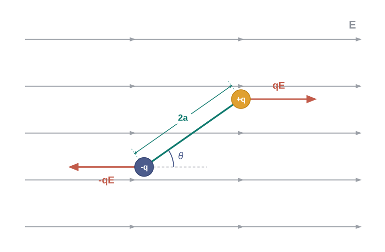
Fig. 1.24 – Dipole in a uniform external field.
Net force is zero, but there is a torque
The charge \(+q\) experiences a force \(q\vec{E}\) in the direction of the field, and the charge \(-q\) experiences a force \(-q\vec{E}\) in the opposite direction. Since the field is uniform, these two forces are equal in magnitude and opposite in direction, so the net force on the dipole is zero.
But that is not the whole story. Although the forces cancel, they do not act at the same point — one acts at \(+q\) and the other at \(-q\), which are separated in space. Two equal and opposite forces acting along different lines form what is called a couple, and a couple produces a turning effect, or torque, on the dipole. (When the net force is zero, this torque is the same about any origin, which is a useful simplification.)
The magnitude of the torque equals the magnitude of one of the forces multiplied by the arm of the couple — the perpendicular distance between the two antiparallel forces. If the dipole makes an angle \(\theta\) with the field, the two charges are separated by \(2a\) along the dipole axis, and the perpendicular distance between the lines of the two forces works out to \(2a\sin\theta\). So the magnitude of the torque is
\[\text{Torque} = qE \times 2a\sin\theta = 2,q,a,E\sin\theta\]
Its direction is perpendicular to the plane of the paper, pointing out of it.
Torque as a vector: \(\vec{\tau} = \vec{p}\times\vec{E}\)
Now recall the definition of the dipole moment, \(p = q \times 2a\). Substituting, the torque magnitude becomes \(pE\sin\theta\). This is exactly the magnitude of the cross product \(\vec{p}\times\vec{E}\), and its direction (out of the paper) also matches. So we can write the torque compactly as
\[\vec{\tau} = \vec{p}\times\vec{E} \tag{1.22}\]
Here \(\vec{\tau}\) is the torque in newton metre (N m), \(\vec{p}\) is the dipole moment in coulomb metre (C m), and \(\vec{E}\) is the external field in N C\(^{-1}\).
This torque tends to rotate the dipole so that it lines up with the field \(\vec{E}\). When \(\vec{p}\) is finally aligned with \(\vec{E}\), the angle \(\theta\) becomes zero, \(\sin\theta = 0\), and the torque vanishes — the dipole has reached its balanced orientation.
What happens in a non-uniform field?
The result above — zero net force, but a torque — holds only when the field is uniform. What if the field is not uniform? Then the forces on \(+q\) and \(-q\) are no longer equal, so the net force is not zero. In general there is both a net force and a torque, and the full analysis is complicated. To keep things simple, consider the special cases where \(\vec{p}\) is parallel to \(\vec{E}\) or antiparallel to \(\vec{E}\). In either case the torque is zero (since \(\sin\theta = 0\)), but there is a net force on the dipole because the field is non-uniform.
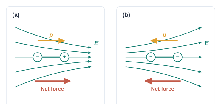
Fig. 1.25 – Dipole in a non-uniform field.
Fig. 1.25 makes this clear. When \(\vec{p}\) is parallel to \(\vec{E}\), the dipole feels a net force in the direction of increasing field. When \(\vec{p}\) is antiparallel to \(\vec{E}\), the net force is in the direction of decreasing field. In general, the force depends on how the dipole is oriented with respect to the field.
Explaining the comb-and-paper puzzle
This finally explains a familiar observation. A comb run through dry hair can attract small pieces of paper — yet the paper carries no net charge. How can an uncharged object be attracted?
The comb, charged by friction, sets up an electric field. This field polarises each piece of paper: it pulls the paper’s positive and negative charges slightly apart, inducing a net dipole moment in the paper, pointing along the field. Now, crucially, the field of the comb is not uniform — it is stronger near the comb and weaker farther away. As we just saw, a dipole in a non-uniform field feels a net force. The induced dipole in the paper is therefore pulled toward the region of stronger field — that is, toward the comb. And so the paper moves toward the comb, even though it began with no charge of its own.
1.12 Continuous Charge Distribution
Up to now, every situation we have studied involved a set of discrete charges \(q_1, q_2, \ldots, q_n\) — separate, countable point charges. One reason for sticking to discrete charges is that the mathematics is simpler and does not require calculus.
For many real problems, however, working with individual charges is hopeless. Think of the surface of a charged conductor. It carries an enormous number of charged particles, and it would be impractical — indeed impossible — to specify the charge by listing the location of every single microscopic charge. In such cases, we treat the charge as if it were spread out smoothly and continuously, and describe it using a charge density.
Surface charge density
Consider a small area element \(\Delta S\) on the surface of the conductor, as in Fig. 1.26. This element is chosen small on the everyday (macroscopic) scale, yet still large enough to contain a very large number of electrons. Let \(\Delta Q\) be the charge on this element. We define the surface charge density \(\sigma\) at this element as
\[\sigma = \frac{\Delta Q}{\Delta S} \tag{1.23}\]
where \(\Delta Q\) is the charge in coulombs (C) and \(\Delta S\) is the area in square metres (m\(^2\)), so \(\sigma\) is measured in C/m\(^2\).
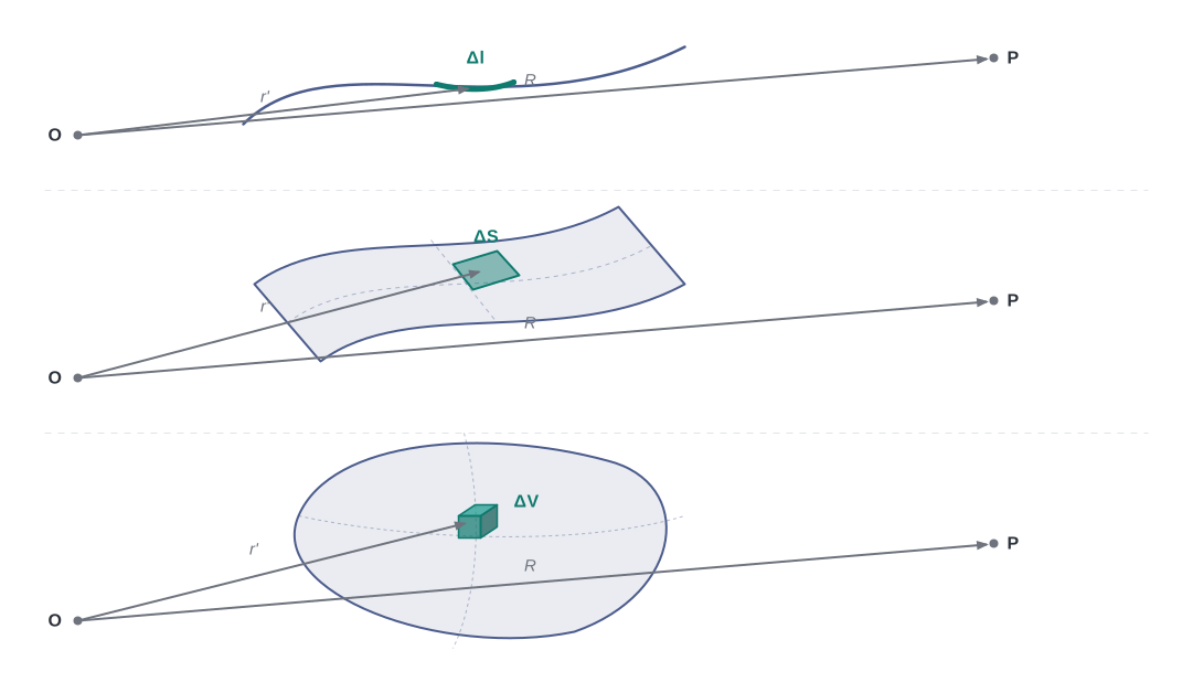
Fig. 1.26 – Continuous charge distributions.
By doing this at different points, we build up a continuous function \(\sigma\), the surface charge density over the whole surface. This \(\sigma\) deliberately ignores the quantisation of charge and the tiny gaps between individual charges at the microscopic level. It represents a macroscopic surface charge density — in effect, a smoothed-out average of the true, grainy microscopic charge density over an area element that is large on the atomic scale but small on the everyday scale.
Linear and volume charge densities
The same idea applies to charge spread along a line or throughout a volume. For a charged wire, the linear charge density \(\lambda\) is defined as
\[\lambda = \frac{\Delta Q}{\Delta l} \tag{1.24}\]
where \(\Delta l\) is a small length element of the wire (small macroscopically, but still containing many charges) and \(\Delta Q\) is the charge on it. The units of \(\lambda\) are C/m.
For charge spread throughout a volume, the volume charge density \(\rho\) (sometimes simply called the charge density) is
\[\rho = \frac{\Delta Q}{\Delta V} \tag{1.25}\]
where \(\Delta Q\) is the charge in a macroscopically small volume element \(\Delta V\) that still contains a large number of charges. The units of \(\rho\) are C/m\(^3\).
This idea of a continuous charge distribution is much like the continuous mass distribution we use in mechanics. When we speak of the density of a liquid, we mean its macroscopic density — we treat the liquid as a continuous fluid and ignore the fact that it is really made of separate molecules.
Field of a continuous distribution
We can find the electric field of a continuous charge distribution in much the same way as for discrete charges, using Eq. (1.10) as our guide. Suppose the distribution has a charge density \(\rho\) that may vary from point to point — that is, \(\rho\) is a function of position. Choose a convenient origin O, and divide the charge distribution into small volume elements of size \(\Delta V\). The charge in each such element is \(\rho,\Delta V\).
Now take any general point P, whether inside or outside the distribution, with position vector \(\vec{R}\), as in Fig. 1.26. By Coulomb’s law, the field at P due to the small charge \(\rho,\Delta V\) is
\[\Delta\vec{E} = \frac{1}{4\pi\varepsilon_0}\frac{\rho,\Delta V}{r'^2},\hat{r}' \tag{1.26}\]
where \(r'\) is the distance between the charge element and P, and \(\hat{r}'\) is the unit vector pointing from the charge element toward P.
By the superposition principle, the total field at P is the sum of the contributions from all the volume elements:
\[\vec{E} \cong \frac{1}{4\pi\varepsilon_0}\sum_{\text{all }\Delta V}\frac{\rho,\Delta V}{r'^2},\hat{r}' \tag{1.27}\]
Note that \(\rho\), \(r'\), and \(\hat{r}'\) can all change from one element to another. In a strict mathematical treatment, we let \(\Delta V \to 0\), and the sum becomes an integral over the whole distribution. We omit that calculus here for simplicity.
The important message is this: using just Coulomb’s law and the superposition principle, we can in principle determine the electric field for any charge distribution — discrete, continuous, or a mixture of both.
1.13 Gauss’s Law
We now use the idea of electric flux to arrive at one of the most elegant and useful results in electrostatics: Gauss’s law. It relates the total flux through a closed surface to the charge enclosed inside it — and remarkably, the shape of the surface does not matter at all.
Flux through a sphere around a point charge
Let us begin with a simple case: the total flux through a sphere of radius \(r\) that encloses a point charge \(q\) at its centre. We divide the sphere into many small area elements, as in Fig. 1.27.
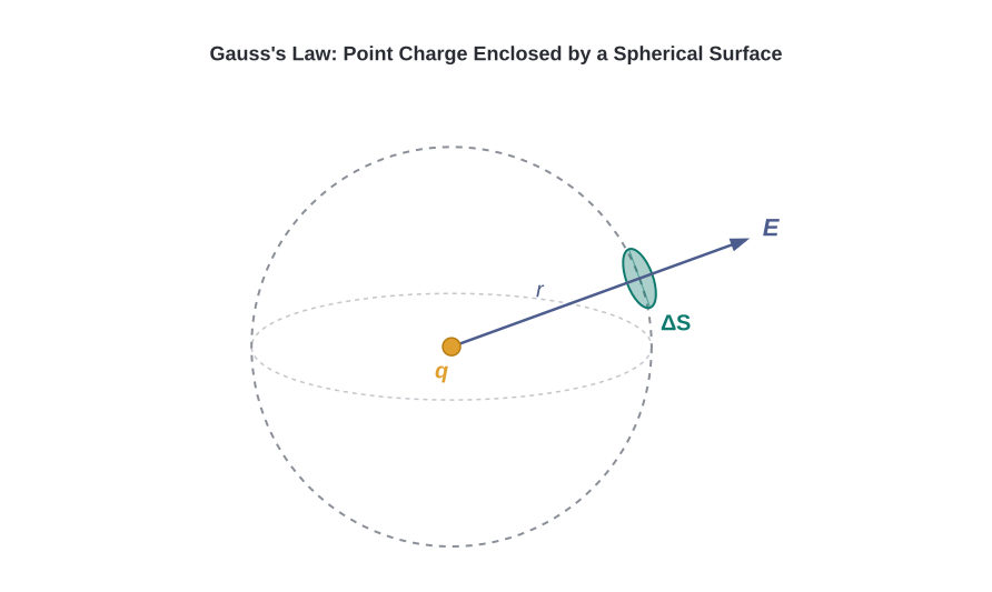
Fig. 1.27 – Flux through a sphere around a point charge.
The flux through one area element \(\Delta\vec{S}\) is
\[\Delta\phi = \vec{E}\cdot\Delta\vec{S} = \frac{q}{4\pi\varepsilon_0 r^2},\hat{r}\cdot\Delta\vec{S} \tag{1.28}\]
where we have used Coulomb’s law for the field of a single charge \(q\), and \(\hat{r}\) is the unit vector along the radius, pointing from the centre to the area element. Now here is the key geometric fact: the normal to a sphere at every point is along the radius. So the area vector \(\Delta\vec{S}\) and \(\hat{r}\) point in the same direction, and their dot product is just \(\Delta S\) (since the angle between them is zero and \(|\hat{r}| = 1\)):
\[\Delta\phi = \frac{q}{4\pi\varepsilon_0 r^2},\Delta S \tag{1.29}\]
To get the total flux, we add up the contributions from all the area elements:
\[\phi = \sum_{\text{all }\Delta S}\frac{q}{4\pi\varepsilon_0 r^2},\Delta S\]
Since every element is at the same distance \(r\) from the charge, the factor \(\dfrac{q}{4\pi\varepsilon_0 r^2}\) is the same for all of them and can be taken outside the sum:
\[\phi = \frac{q}{4\pi\varepsilon_0 r^2}\sum_{\text{all }\Delta S}\Delta S = \frac{q}{4\pi\varepsilon_0 r^2},S\]
The sum of all the area elements is just \(S\), the total surface area of the sphere, which is \(4\pi r^2\). Substituting,
\[\phi = \frac{q}{4\pi\varepsilon_0 r^2}\times 4\pi r^2 = \frac{q}{\varepsilon_0} \tag{1.30}\]
Notice something striking: the radius \(r\) has completely cancelled out. The total flux depends only on the enclosed charge \(q\) and the constant \(\varepsilon_0\) — not on the size of the sphere.
Statement of Gauss’s law
Equation (1.30) is a simple illustration of a far more general result called Gauss’s law, which we state here without proof:
A direct consequence is that if no charge is enclosed by a closed surface, the total flux through it is zero. We can see this explicitly in the simple situation of Fig. 1.28.
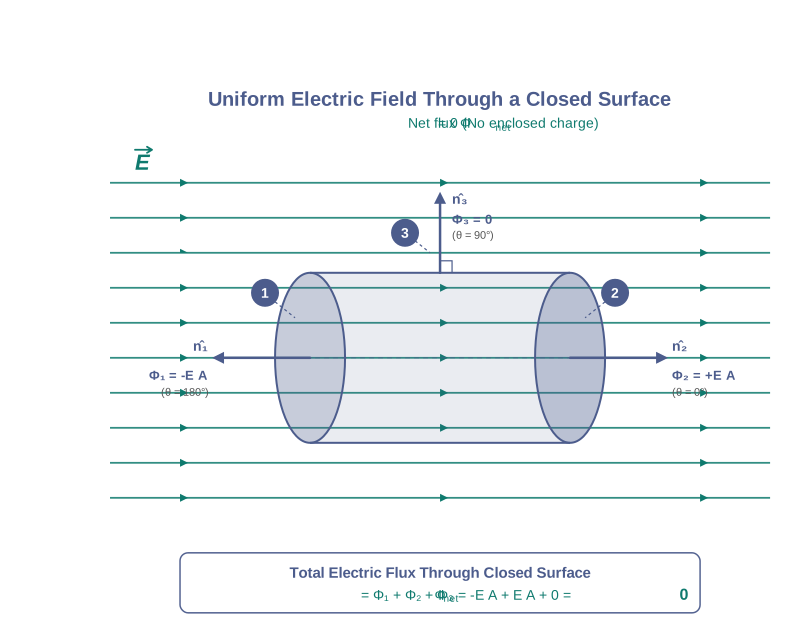
Fig. 1.28 – Net flux through a cylinder in a uniform field.
Here the field is uniform, and we take a closed cylindrical surface with its axis parallel to the field \(\vec{E}\). The total flux is \(\phi = \phi_1 + \phi_2 + \phi_3\), where \(\phi_1\) and \(\phi_2\) are the fluxes through the two flat circular faces (1 and 2), and \(\phi_3\) is the flux through the curved side of the cylinder. On the curved side, the normal is everywhere perpendicular to \(\vec{E}\), so \(\phi_3 = 0\). On face 2, the outward normal is along \(\vec{E}\), while on face 1 it points opposite to \(\vec{E}\). Therefore
\[\phi_1 = -E,S_1, \qquad \phi_2 = +E,S_2, \qquad S_1 = S_2 = S\]
so the two contributions cancel and the total flux is zero — exactly as Gauss’s law requires, since no charge is enclosed. In general, whenever you find that the net flux through a closed surface is zero, you can conclude that the total charge enclosed is zero.
Important points about Gauss’s law
The real power of Gauss’s law is that it holds in general, not just in the simple cases above. A few points are worth noting carefully:
Gauss’s law is true for any closed surface, no matter what its shape or size.
The charge \(q\) on the right-hand side is the sum of all charges enclosed by the surface. These charges may be located anywhere inside the surface.
If the surface encloses some charges while others lie outside it, then the field \(\vec{E}\) on the left-hand side (whose flux we compute) is due to all the charges, both inside and outside. But the charge \(q\) on the right-hand side represents only the total charge inside the surface.
The surface we choose for applying Gauss’s law is called the Gaussian surface. You may choose any Gaussian surface you like — but take care not to let it pass through any discrete (point) charge, because the field is not well defined at the exact location of a point charge (it grows without bound there). A Gaussian surface may, however, pass through a continuous charge distribution.
- Gauss’s law is especially useful for calculating the electric field easily when the charge distribution has some symmetry. This is done by choosing a Gaussian surface that matches the symmetry of the problem.
- Finally, Gauss’s law rests on the inverse-square dependence on distance contained in Coulomb’s law. Any experimental violation of Gauss’s law would signal a departure from the inverse-square law.
The electric field components in Fig. 1.29 are \(E_x = \alpha x^{1/2}\), \(E_y = E_z = 0\), where \(\alpha = 800\) N/C m\(^{1/2}\). Calculate (a) the flux through the cube, and (b) the charge within the cube. Take the side of the cube to be \(a = 0.1\) m.
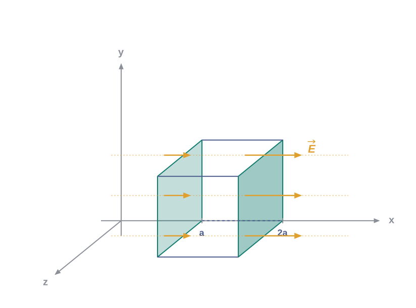
[Caption:] Fig. 1.29 – Flux through a cube in a non-uniform field. [/Caption:]
Since the field points only along \(x\), only the two faces perpendicular to \(x\) have any flux. We compute the flux through each, add them, then use Gauss’s law to find the enclosed charge.
- Because the field has only an \(x\)-component, on the four faces perpendicular to the \(y\) and \(z\) directions the angle between \(\vec{E}\) and \(\Delta\vec{S}\) is \(\pm\pi/2\), so the flux \(\phi = \vec{E}\cdot\Delta\vec{S}\) is zero on each of them. Only the two shaded faces (perpendicular to \(x\)) contribute.
The magnitude of the field at the left face (where \(x = a\)) is
\[E_L = \alpha x^{1/2} = \alpha a^{1/2}\]
and at the right face (where \(x = 2a\)) is
\[E_R = \alpha x^{1/2} = \alpha (2a)^{1/2}\]
The corresponding fluxes are
\[\phi_L = \vec{E}_L\cdot\Delta\vec{S} = E_L,\Delta S\cos\theta = -E_L,\Delta S = -E_L,a^2 \qquad (\theta = 180^\circ)\]
\[\phi_R = \vec{E}_R\cdot\Delta\vec{S} = E_R,\Delta S\cos\theta = E_R,\Delta S = E_R,a^2 \qquad (\theta = 0^\circ)\]
So the net flux through the cube is
\[\phi = \phi_R + \phi_L = E_R,a^2 - E_L,a^2 = a^2(E_R - E_L) = \alpha a^2\left[(2a)^{1/2} - a^{1/2}\right]\]
\[= \alpha a^{5/2}\left(\sqrt{2} - 1\right) = 800 \times (0.1)^{5/2}\left(\sqrt{2} - 1\right) = 1.05 \ \text{N m}^2,\text{C}^{-1}\]
- By Gauss’s law, \(\phi = q/\varepsilon_0\), so \(q = \phi,\varepsilon_0\). Therefore
\[q = 1.05 \times 8.854 \times 10^{-12} \ \text{C} = 9.27 \times 10^{-12} \ \text{C}\]
An electric field is uniform and points in the \(+x\) direction for positive \(x\), and is uniform with the same magnitude but points in the \(-x\) direction for negative \(x\). That is, \(\vec{E} = 200,\hat{i}\) N/C for \(x > 0\) and \(\vec{E} = -200,\hat{i}\) N/C for \(x < 0\). A right circular cylinder of length \(20\) cm and radius \(5\) cm has its centre at the origin and its axis along the \(x\)-axis, so that one face is at \(x = +10\) cm and the other at \(x = -10\) cm (Fig. 1.30). Find (a) the net outward flux through each flat face, (b) the flux through the side of the cylinder, (c) the net outward flux through the cylinder, and (d) the net charge inside the cylinder.
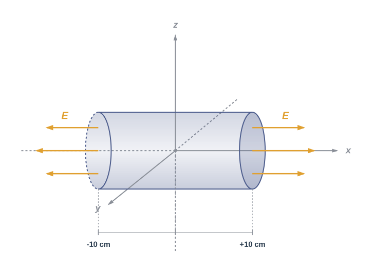
[Caption:] Fig. 1.30 – Cylinder in a field pointing outward from both faces. [/Caption:]
The field is along the axis, so only the flat faces have flux. We add the flux through both faces, then apply Gauss’s law for the enclosed charge.
- On the left face, \(\vec{E}\) and \(\Delta\vec{S}\) are parallel (both point outward, in the \(-x\) direction). The outward flux is
\[\phi_L = \vec{E}\cdot\Delta\vec{S} = -200,\hat{i}\cdot\Delta\vec{S} = +200,\Delta S \qquad (\text{since }\hat{i}\cdot\Delta\vec{S} = -\Delta S)\]
\[= +200 \times \pi(0.05)^2 = +1.57 \ \text{N m}^2,\text{C}^{-1}\]
On the right face, \(\vec{E}\) and \(\Delta\vec{S}\) are again parallel, so
\[\phi_R = \vec{E}\cdot\Delta\vec{S} = +1.57 \ \text{N m}^2,\text{C}^{-1}\]
On the curved side of the cylinder, \(\vec{E}\) is perpendicular to \(\Delta\vec{S}\), so \(\vec{E}\cdot\Delta\vec{S} = 0\). The flux through the side is zero.
The net outward flux through the cylinder is
\[\phi = 1.57 + 1.57 + 0 = 3.14 \ \text{N m}^2,\text{C}^{-1}\]
- By Gauss’s law, the net charge inside is
\[q = \varepsilon_0\phi = 3.14 \times 8.854 \times 10^{-12} \ \text{C} = 2.78 \times 10^{-11} \ \text{C}\]
1.14 Applications of Gauss’s Law
We have seen that the field due to a general charge distribution is given by Eq. (1.27). But in practice, except for a few special cases, the summation (or integration) in that equation cannot actually be carried out to give the field at every point in space. This is where Gauss’s law becomes a powerful shortcut. For charge distributions that have some symmetry, Gauss’s law lets us find the field simply and elegantly. The method is best understood through examples, and we now work through three important ones.
The strategy in each case is the same: use the symmetry of the charge distribution to argue what direction the field points and what it depends on, then choose a Gaussian surface that matches this symmetry so that the flux integral becomes trivial.
1.14.1 Field due to an infinitely long straight uniformly charged wire
Consider an infinitely long, thin, straight wire with a uniform linear charge density \(\lambda\). Such a wire is an axis of symmetry: if we take the radial line from a point O on the wire out to a point P, and rotate it around the wire, the points P, P′, P″ we reach are all completely equivalent with respect to the charged wire.
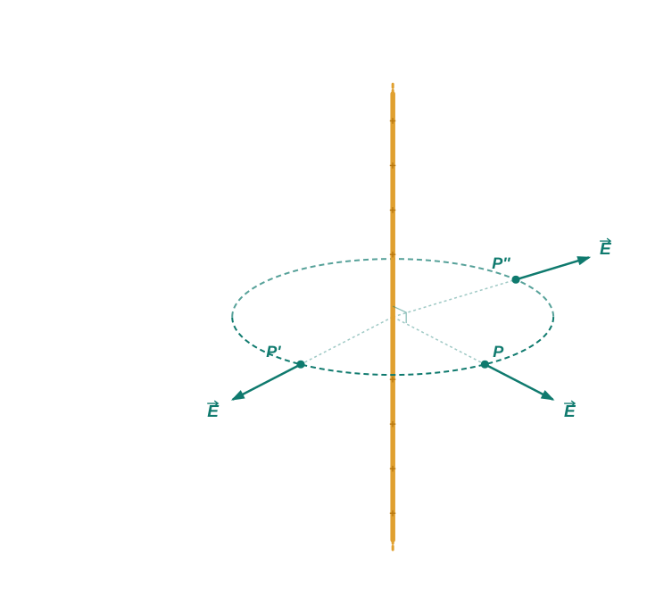
Fig. 1.31(a) – Field symmetry around a long charged wire.
This symmetry tells us two things. First, the field must have the same magnitude at all these points. Second, the field must point radially — outward if \(\lambda > 0\), inward if \(\lambda < 0\).
To see why the field is purely radial, consider a pair of small line elements \(P_1\) and \(P_2\) of the wire, placed symmetrically. When we add the fields from this pair, the components perpendicular to the radial direction cancel, leaving only a radial resultant. This holds for every such pair, so the total field at P is radial. And because the wire is infinite, the field cannot depend on where P lies along the length of the wire. In short, the field is everywhere radial in the plane cutting the wire at right angles, and its magnitude depends only on the radial distance \(r\) from the wire.
Choosing the Gaussian surface
To calculate the field, we choose a cylindrical Gaussian surface of radius \(r\) and length \(l\), coaxial with the wire, as in Fig. 1.31(b).
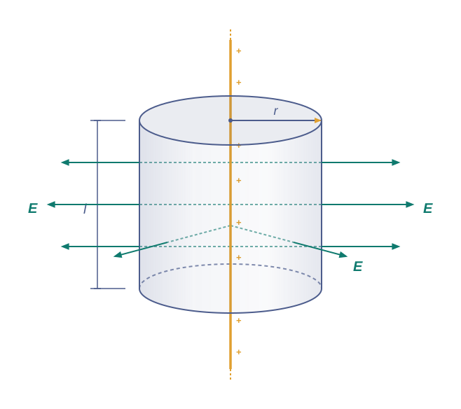
Fig. 1.31(b) – Gaussian surface for a charged wire.
Since the field is everywhere radial, it is parallel to the flat end faces of the cylinder, so the flux through the two ends is zero. On the curved cylindrical part, the field \(\vec{E}\) is normal to the surface at every point, and its magnitude is constant (it depends only on \(r\)). The surface area of the curved part is \(2\pi r l\).
So the total flux through the Gaussian surface equals the flux through the curved part:
\[\phi = E \times 2\pi r l\]
The charge enclosed by this surface is the charge on the length \(l\) of wire, which is \(\lambda l\). Applying Gauss’s law, \(\phi = q/\varepsilon_0\):
\[E \times 2\pi r l = \frac{\lambda l}{\varepsilon_0}\]
The length \(l\) cancels, giving
\[E = \frac{\lambda}{2\pi\varepsilon_0 r}\]
In vector form, the field at any point is
\[\vec{E} = \frac{\lambda}{2\pi\varepsilon_0 r},\hat{n} \tag{1.32}\]
where \(\hat{n}\) is the radial unit vector in the plane normal to the wire, passing through the point. The field points outward if \(\lambda\) is positive and inward if \(\lambda\) is negative. Notice that for a line charge the field falls off as \(1/r\), not \(1/r^2\).
A short note on notation: when we write a vector as \(\vec{A} = A,\hat{a}\), the scalar \(A\) is an algebraic number that can be positive or negative. The direction of \(\vec{A}\) is the same as \(\hat{a}\) if \(A > 0\), and opposite to \(\hat{a}\) if \(A < 0\). When we want to restrict to non-negative values only, we write \(|\vec{A}|\), the modulus, with \(|\vec{A}| \geq 0\).
1.14.2 Field due to a uniformly charged infinite plane sheet
Now let \(\sigma\) be the uniform surface charge density of an infinite plane sheet, as in Fig. 1.32. We take the \(x\)-axis normal to the sheet. By symmetry, the field cannot depend on the \(y\) and \(z\) coordinates (the sheet looks the same in every direction along its surface), and its direction at every point must be parallel to the \(x\)-axis — straight out from the sheet.
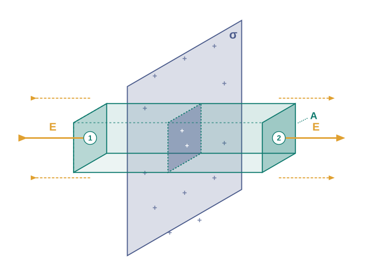
Fig. 1.32 – Gaussian surface for an infinite charged sheet.
Choosing the Gaussian surface
We take the Gaussian surface to be a rectangular box (a parallelepiped) of cross-sectional area \(A\), pierced symmetrically by the sheet. (A cylinder would work equally well.) Only the two faces parallel to the sheet — faces 1 and 2 — contribute to the flux; the field lines are parallel to the other faces, so those contribute nothing.
The outward normal to face 1 is in the \(-x\) direction and that to face 2 is in the \(+x\) direction. On both faces the field points outward along the normal, so the two fluxes are equal and add up. The net flux through the Gaussian surface is therefore
\[\phi = 2EA\]
The charge enclosed by the box is the charge on the area \(A\) of the sheet, which is \(\sigma A\). Applying Gauss’s law:
\[2EA = \frac{\sigma A}{\varepsilon_0}\]
so that
\[E = \frac{\sigma}{2\varepsilon_0}\]
In vector form,
\[\vec{E} = \frac{\sigma}{2\varepsilon_0},\hat{n} \tag{1.33}\]
where \(\hat{n}\) is the unit vector normal to the sheet, pointing away from it. The field points away from the sheet if \(\sigma\) is positive, and toward it if \(\sigma\) is negative.
There is a remarkable feature here: the field does not depend on \(x\) at all. In other words, the field of an infinite charged sheet is uniform — the same magnitude at every distance from the sheet. For a real, finite sheet, Eq. (1.33) holds approximately in the middle region, away from the edges.
1.14.3 Field due to a uniformly charged thin spherical shell
Finally, let \(\sigma\) be the uniform surface charge density of a thin spherical shell of radius \(R\), as in Fig. 1.33. This situation has obvious spherical symmetry. The field at any point P — whether outside or inside the shell — can depend only on \(r\), the radial distance from the centre of the shell, and must point radially (along the radius vector).
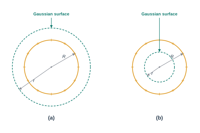
Fig. 1.33 – Gaussian spheres for a charged shell.
(i) Field outside the shell. Consider a point P outside the shell, at distance \(r\) from the centre. We take the Gaussian surface to be a sphere of radius \(r\) centred at O, passing through P. By spherical symmetry, all points on this sphere are equivalent, so the field has the same magnitude \(E\) everywhere on it and points radially. Thus \(\vec{E}\) and \(\Delta\vec{S}\) are parallel at every point, and the flux through each element is \(E,\Delta S\). Summing over the whole sphere gives a total flux
\[\phi = E \times 4\pi r^2\]
The charge enclosed by this Gaussian sphere is the entire charge of the shell, \(\sigma \times 4\pi R^2\). By Gauss’s law,
\[E \times 4\pi r^2 = \frac{\sigma \times 4\pi R^2}{\varepsilon_0}\]
Solving,
\[E = \frac{\sigma R^2}{\varepsilon_0 r^2} = \frac{q}{4\pi\varepsilon_0 r^2}\]
where \(q = 4\pi R^2\sigma\) is the total charge on the shell. In vector form,
\[\vec{E} = \frac{q}{4\pi\varepsilon_0 r^2},\hat{r} \tag{1.34}\]
The field points outward if \(q > 0\) and inward if \(q < 0\). But look closely at this result: it is exactly the field that would be produced by a point charge \(q\) sitting at the centre O. So for all points outside the shell, the uniformly charged shell behaves as if its entire charge were concentrated at its centre.
(ii) Field inside the shell. Now consider a point P inside the shell, as in Fig. 1.33(b). We again take the Gaussian surface to be a sphere through P centred at O. The flux is still \(E \times 4\pi r^2\). But this time the Gaussian surface encloses no charge at all (all the charge sits on the shell of radius \(R\), which is outside our inner sphere). So Gauss’s law gives
\[E \times 4\pi r^2 = 0\]
that is,
\[E = 0 \qquad (r < R) \tag{1.35}\]
The field due to a uniformly charged thin shell is zero everywhere inside the shell. This is a direct and important consequence of Gauss’s law, which in turn follows from Coulomb’s law. In fact, the experimental confirmation that the field inside is exactly zero is one of the most sensitive tests of the \(1/r^2\) dependence in Coulomb’s law.
An early model of the atom pictured it as a positively charged point nucleus of charge \(Ze\), surrounded by a uniform density of negative charge extending out to a radius \(R\). The atom as a whole is neutral. For this model, find the electric field at a distance \(r\) from the nucleus.
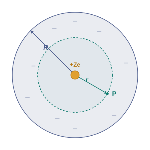
[Caption:] Fig. 1.34 – Early model of an atom. [/Caption:]
First find the negative charge density from the neutrality condition, then apply Gauss’s law separately for a point inside (\(r < R\)) and outside (\(r > R\)) the negative cloud.
The charge distribution is shown in Fig. 1.34. Since the atom is neutral, the total negative charge in the uniform sphere of radius \(R\) must be \(-Ze\) (to cancel the nuclear charge \(+Ze\)). This fixes the negative charge density \(\rho\): the volume of the sphere times \(\rho\) must equal \(-Ze\),
\[\frac{4\pi R^3}{3},\rho = 0 - Ze\]
so
\[\rho = -\frac{3Ze}{4\pi R^3}\]
To find the field \(\vec{E}(r)\) at a point P a distance \(r\) from the nucleus, we use Gauss’s law. Because of the spherical symmetry, the magnitude of \(\vec{E}(r)\) depends only on \(r\), and its direction is along (or opposite to) the radius vector. The natural Gaussian surface is a sphere centred at the nucleus. We consider the two cases \(r < R\) and \(r > R\).
(i) For \(r < R\): The electric flux through the Gaussian sphere is
\[\phi = E(r) \times 4\pi r^2\]
since the field has the same magnitude and is normal to the surface everywhere on it. The charge \(q\) enclosed by this sphere is the positive nuclear charge plus the negative charge lying within the sphere of radius \(r\):
\[q = Ze + \frac{4\pi r^3}{3},\rho\]
Substituting the value of \(\rho\) found above,
\[q = Ze - Ze,\frac{r^3}{R^3}\]
Gauss’s law, \(E(r)\times 4\pi r^2 = q/\varepsilon_0\), then gives
\[E(r) = \frac{Ze}{4\pi\varepsilon_0}\left(\frac{1}{r^2} - \frac{r}{R^3}\right); \qquad r < R\]
and the field is directed radially outward.
(ii) For \(r > R\): Now the Gaussian sphere encloses the whole atom, whose total charge is zero (the atom is neutral). So Gauss’s law gives
\[E(r) \times 4\pi r^2 = 0 \qquad \text{or} \qquad E(r) = 0; \qquad r > R\]
At the boundary \(r = R\), both expressions give the same result, \(E = 0\), so the field is continuous there.
1.15 Summary
Electric and magnetic forces determine the properties of atoms, molecules, and bulk matter.
Simple experiments on frictional electricity show that there are two kinds of charge in nature, and that like charges repel while unlike charges attract. By convention, the charge on a glass rod rubbed with silk is positive, and that on a plastic rod rubbed with fur is negative.
Conductors allow electric charge to move through them, while insulators do not. In metals the mobile charges are electrons; in electrolytes, both positive and negative ions are mobile.
Electric charge has three basic properties: quantisation, additivity, and conservation.
Quantisation means that the total charge \(q\) of a body is always an integer multiple of the basic quantum of charge \(e\); that is, \(q = ne\), where \(n = 0, \pm1, \pm2, \pm3, \ldots\). The proton and electron carry charges \(+e\) and \(-e\) respectively. For macroscopic charges, \(n\) is so large that quantisation can be ignored.
Additivity means the total charge of a system is the algebraic sum (taking signs into account) of all the individual charges in the system.
Conservation means the total charge of an isolated system stays unchanged with time. When bodies are charged by friction, charge is only transferred from one body to another — none is created or destroyed.
Coulomb’s law: the mutual electrostatic force between two point charges \(q_1\) and \(q_2\) is proportional to the product \(q_1 q_2\) and inversely proportional to the square of the distance \(r_{21}\) separating them:
\[\vec{F}*{21} = \frac{k,(q_1 q_2)}{r*{21}^2},\hat{r}_{21}\]
where \(\hat{r}_{21}\) is the unit vector from \(q_1\) to \(q_2\), and \(k = \dfrac{1}{4\pi\varepsilon_0}\) is the constant of proportionality. In SI units the unit of charge is the coulomb, and
\[\varepsilon_0 = 8.854 \times 10^{-12} \ \text{C}^2,\text{N}^{-1},\text{m}^{-2}, \qquad k \approx 9 \times 10^{9} \ \text{N m}^2,\text{C}^{-2}\]
The ratio of the electric force to the gravitational force between a proton and an electron is
\[\frac{k e^2}{G, m_e m_p} \cong 2.4 \times 10^{39}\]
Superposition principle: the force with which two charges attract or repel each other is not affected by the presence of any additional charges. So for an assembly of charges, the total force on any one charge is the vector sum of the forces due to each of the other charges taken one at a time, each given by Coulomb’s law.
The electric field \(\vec{E}\) at a point due to a charge configuration is the force on a small positive test charge \(q\) placed there, divided by the magnitude of that charge. The field due to a point charge \(q\) has magnitude \(|q|/(4\pi\varepsilon_0 r^2)\); it points radially outward if \(q\) is positive and radially inward if \(q\) is negative. Like the Coulomb force, the electric field obeys the superposition principle.
An electric field line is a curve whose tangent at each point gives the direction of the electric field at that point. The relative closeness of the field lines shows the relative strength of the field — they crowd together where the field is strong and spread apart where it is weak. In a region of constant field, the lines are uniformly spaced parallel straight lines.
Important properties of field lines: (i) they are continuous curves without breaks; (ii) two field lines can never cross each other; (iii) electrostatic field lines start at positive charges and end at negative charges, and they cannot form closed loops.
An electric dipole is a pair of equal and opposite charges \(q\) and \(-q\) separated by a distance \(2a\). Its dipole moment vector \(\vec{p}\) has magnitude \(2qa\) and points along the dipole axis, from \(-q\) to \(q\).
The field of a dipole in its equatorial plane (perpendicular to the axis, through the centre) at distance \(r\) from the centre is
\[\vec{E} = \frac{-\vec{p}}{4\pi\varepsilon_0}\frac{1}{(a^2 + r^2)^{3/2}} \cong \frac{-\vec{p}}{4\pi\varepsilon_0 r^3}, \qquad \text{for } r \gg a\]
The dipole field on the axis at distance \(r\) from the centre is
\[\vec{E} = \frac{2\vec{p},r}{4\pi\varepsilon_0 (r^2 - a^2)^2} \cong \frac{2\vec{p}}{4\pi\varepsilon_0 r^3}, \qquad \text{for } r \gg a\]
The \(1/r^3\) dependence of dipole fields should be noted, in contrast to the \(1/r^2\) dependence of the field due to a point charge.
- In a uniform electric field \(\vec{E}\), a dipole experiences a torque \(\vec{\tau}\) given by
\[\vec{\tau} = \vec{p}\times\vec{E}\]
but experiences no net force.
- The flux \(\Delta\phi\) of the electric field \(\vec{E}\) through a small area element \(\Delta\vec{S}\) is
\[\Delta\phi = \vec{E}\cdot\Delta\vec{S}\]
The vector area element is \(\Delta\vec{S} = \Delta S,\hat{n}\), where \(\Delta S\) is the magnitude of the element and \(\hat{n}\) is normal to it (the element may be treated as planar for sufficiently small \(\Delta S\)). For an element of a closed surface, \(\hat{n}\) is taken along the outward normal, by convention.
- Gauss’s law: the flux of the electric field through any closed surface \(S\) equals \(\dfrac{1}{\varepsilon_0}\) times the total charge enclosed by \(S\). The law is especially useful for finding the field when the source distribution has simple symmetry:
- For a thin, infinitely long straight wire of uniform linear charge density \(\lambda\):
\[\vec{E} = \frac{\lambda}{2\pi\varepsilon_0 r},\hat{n}\]
where \(r\) is the perpendicular distance of the point from the wire and \(\hat{n}\) is the radial unit vector in the plane normal to the wire.
- For an infinite thin plane sheet of uniform surface charge density \(\sigma\):
\[\vec{E} = \frac{\sigma}{2\varepsilon_0},\hat{n}\]
where \(\hat{n}\) is the unit vector normal to the plane, pointing outward on either side.
- For a thin spherical shell of uniform surface charge density \(\sigma\):
\[\vec{E} = \frac{q}{4\pi\varepsilon_0 r^2},\hat{r} \quad (r \geq R), \qquad \vec{E} = 0 \quad (r < R)\]
where \(r\) is the distance of the point from the centre of the shell, \(R\) is the radius of the shell, and \(q = 4\pi R^2\sigma\) is the total charge on the shell. Outside the shell the field is as though the total charge were concentrated at the centre; the same result holds for a solid sphere of uniform volume charge density. The field is zero at all points inside the shell.
Table of physical quantities
| Physical quantity | Symbol | Dimensions | Unit | Remarks |
|---|---|---|---|---|
| Vector area element | \(\Delta\vec{S}\) | \([\text{L}^2]\) | m\(^2\) | \(\Delta\vec{S} = \Delta S,\hat{n}\) |
| Electric field | \(\vec{E}\) | \([\text{MLT}^{-3}\text{A}^{-1}]\) | V m\(^{-1}\) | |
| Electric flux | \(\phi\) | \([\text{ML}^3\text{T}^{-3}\text{A}^{-1}]\) | V m | \(\Delta\phi = \vec{E}\cdot\Delta\vec{S}\) |
| Dipole moment | \(\vec{p}\) | \([\text{LTA}]\) | C m | Vector directed from negative to positive charge |
| Charge density (linear) | \(\lambda\) | \([\text{L}^{-1}\text{TA}]\) | C m\(^{-1}\) | Charge/length |
| Charge density (surface) | \(\sigma\) | \([\text{L}^{-2}\text{TA}]\) | C m\(^{-2}\) | Charge/area |
| Charge density (volume) | \(\rho\) | \([\text{L}^{-3}\text{TA}]\) | C m\(^{-3}\) | Charge/volume |
1.16 Points to Ponder
- You might wonder why the protons, all carrying positive charge, sit packed so closely together inside the nucleus without flying apart. From Coulomb’s law, they should repel one another very strongly. The answer is that there is a third kind of fundamental force, called the strong force, which holds them together. This force is effective only over an extremely small range, about \(10^{-14}\) m — which is precisely the size of the nucleus. Also, the electrons are not allowed to sit right on top of the protons, inside the nucleus, because of the laws of quantum mechanics. Together, these facts give atoms the structure they have in nature.
- The Coulomb force and the gravitational force follow the same inverse-square law. But gravity has only one sign — it is always attractive — while the Coulomb force comes in both signs (attractive and repulsive), which allows electric forces to cancel. This is why gravity, even though it is a far weaker force, can end up being the dominant, more far-reaching force on large scales: there is no cancellation to weaken it.
- The constant of proportionality \(k\) in Coulomb’s law is a matter of choice, if the unit of charge is defined using Coulomb’s law itself. In SI units, however, it is the unit of current (the ampere) that is defined first, through its magnetic effect (Ampère’s law), and the unit of charge (the coulomb) is then simply defined by \(1\ \text{C} = 1\ \text{A s}\). In that case the value of \(k\) is no longer arbitrary; it comes out to be approximately \(9 \times 10^{9}\) N m\(^2\) C\(^{-2}\).
- The rather large value of \(k\) — that is, the large size of the unit of charge (1 C) from the point of view of electric effects — arises because, as noted above, the unit of charge is defined in terms of magnetic forces (forces on current-carrying wires), which are generally much weaker than electric forces. So while 1 ampere is a reasonable-sized unit for magnetic effects, \(1\ \text{C} = 1\ \text{A s}\) turns out to be too big a unit for electric effects.
- The additive property of charge is not an “obvious” property. It is tied to the fact that electric charge has no direction associated with it — charge is a scalar.
- Charge is not only a scalar (invariant under rotation); it is also invariant for observers in relative motion. This is not true of every scalar. For example, kinetic energy is a scalar under rotation, but it is not invariant when we move to a frame of reference in relative motion.
- The conservation of the total charge of an isolated system is a property independent of the scalar nature of charge noted above. Conservation refers to invariance in time in a given frame of reference. A quantity may be a scalar and yet not be conserved (like kinetic energy in an inelastic collision). Conversely, one can have a conserved vector quantity (like the angular momentum of an isolated system).
- The quantisation of electric charge is a basic, so far unexplained, law of nature. Interestingly, there is no analogous law for the quantisation of mass.
- The superposition principle should not be regarded as “obvious,” nor simply equated with the law of addition of vectors. It actually says two separate things: first, the force on one charge due to another is unaffected by the presence of other charges; and second, there are no extra three-body, four-body, or higher forces that appear only when more than two charges are present.
- The electric field due to a discrete charge configuration is not defined at the exact locations of the charges. For a continuous volume charge distribution, the field is defined at every point within the distribution. For a surface charge distribution, the field is discontinuous across the surface.
- The electric field due to a charge configuration with total charge zero is not zero; but at distances large compared with the size of the configuration, it falls off faster than \(1/r^2\), the fall-off typical of a single charge. An electric dipole is the simplest example of this fact.
1.17 NCERT Questions
- What is the force between two small charged spheres having charges of \(2 \times 10^{-7}\) C and \(3 \times 10^{-7}\) C placed \(30\) cm apart in air?
- The electrostatic force on a small sphere of charge \(0.4\ \mu\)C due to another small sphere of charge \(-0.8\ \mu\)C in air is \(0.2\) N. (a) What is the distance between the two spheres? (b) What is the force on the second sphere due to the first?
- Check that the ratio \(ke^2 / G, m_e m_p\) is dimensionless. Look up a table of physical constants and determine the value of this ratio. What does the ratio signify?
- Explain the meaning of the statement ‘electric charge of a body is quantised’. (b) Why can one ignore quantisation of electric charge when dealing with macroscopic, i.e., large-scale, charges?
- When a glass rod is rubbed with a silk cloth, charges appear on both. A similar phenomenon is observed with many other pairs of bodies. Explain how this observation is consistent with the law of conservation of charge.
- Four point charges \(q_A = 2\ \mu\)C, \(q_B = -5\ \mu\)C, \(q_C = 2\ \mu\)C, and \(q_D = -5\ \mu\)C are located at the corners of a square ABCD of side \(10\) cm. What is the force on a charge of \(1\ \mu\)C placed at the centre of the square?
- An electrostatic field line is a continuous curve. That is, a field line cannot have sudden breaks. Why not? (b) Explain why two field lines never cross each other at any point.
- Two point charges \(q_A = 3\ \mu\)C and \(q_B = -3\ \mu\)C are located \(20\) cm apart in vacuum. (a) What is the electric field at the midpoint O of the line AB joining the two charges? (b) If a negative test charge of magnitude \(1.5 \times 10^{-9}\) C is placed at this point, what is the force experienced by the test charge?
- A system has two charges \(q_A = 2.5 \times 10^{-7}\) C and \(q_B = -2.5 \times 10^{-7}\) C located at points A: \((0, 0, -15\) cm\()\) and B: \((0, 0, +15\) cm\()\), respectively. What are the total charge and electric dipole moment of the system?
- An electric dipole with dipole moment \(4 \times 10^{-9}\) C m is aligned at \(30^\circ\) with the direction of a uniform electric field of magnitude \(5 \times 10^{4}\) N C\(^{-1}\). Calculate the magnitude of the torque acting on the dipole.
- A polythene piece rubbed with wool is found to have a negative charge of \(3 \times 10^{-7}\) C. (a) Estimate the number of electrons transferred (from which to which?). (b) Is there a transfer of mass from wool to polythene?
- Two insulated charged copper spheres A and B have their centres separated by a distance of \(50\) cm. What is the mutual force of electrostatic repulsion if the charge on each is \(6.5 \times 10^{-7}\) C? The radii of A and B are negligible compared to the distance of separation. (b) What is the force of repulsion if each sphere is charged double the above amount, and the distance between them is halved?
- Figure 1.35 shows tracks of three charged particles in a uniform electrostatic field. Give the signs of the three charges. Which particle has the highest charge-to-mass ratio?
- Consider a uniform electric field \(\vec{E} = 3 \times 10^{3},\hat{i}\) N/C. (a) What is the flux of this field through a square of side \(10\) cm whose plane is parallel to the \(yz\) plane? (b) What is the flux through the same square if the normal to its plane makes a \(60^\circ\) angle with the \(x\)-axis?
- What is the net flux of the uniform electric field of Question 14 through a cube of side \(20\) cm oriented so that its faces are parallel to the coordinate planes?
- Careful measurement of the electric field at the surface of a black box indicates that the net outward flux through the surface of the box is \(8.0 \times 10^{3}\) N m\(^2\)/C. (a) What is the net charge inside the box? (b) If the net outward flux through the surface of the box were zero, could you conclude that there were no charges inside the box? Why or why not?
- A point charge \(+10\ \mu\)C is a distance \(5\) cm directly above the centre of a square of side \(10\) cm, as shown in Fig. 1.36. What is the magnitude of the electric flux through the square? (Hint: Think of the square as one face of a cube with edge \(10\) cm.)
- A point charge of \(2.0\ \mu\)C is at the centre of a cubic Gaussian surface \(9.0\) cm on edge. What is the net electric flux through the surface?
- A point charge causes an electric flux of \(-1.0 \times 10^{3}\) N m\(^2\)/C to pass through a spherical Gaussian surface of \(10.0\) cm radius centred on the charge. (a) If the radius of the Gaussian surface were doubled, how much flux would pass through the surface? (b) What is the value of the point charge?
- A conducting sphere of radius \(10\) cm has an unknown charge. If the electric field \(20\) cm from the centre of the sphere is \(1.5 \times 10^{3}\) N/C and points radially inward, what is the net charge on the sphere?
- A uniformly charged conducting sphere of \(2.4\) m diameter has a surface charge density of \(80.0\ \mu\)C/m\(^2\). (a) Find the charge on the sphere. (b) What is the total electric flux leaving the surface of the sphere?
- An infinite line charge produces a field of \(9 \times 10^{4}\) N/C at a distance of \(2\) cm. Calculate the linear charge density.
- Two large, thin metal plates are parallel and close to each other. On their inner faces, the plates have surface charge densities of opposite signs and of magnitude \(17.0 \times 10^{-22}\) C/m\(^2\). What is \(\vec{E}\): (a) in the outer region of the first plate, (b) in the outer region of the second plate, and (c) between the plates?
1.18 Check Your Concepts
- While adding masses we never worry about signs, but while adding charges we must. Explain what property of electric charge makes this signed addition necessary, and what would go wrong if signs were ignored.
- A charged metal spoon held in the bare hand shows no sign of charge after rubbing, but the same metal fitted with a wooden handle does. Explain this difference in terms of conductors and insulators.
- The electric field due to a single point charge falls off as \(1/r^2\), while that due to a dipole falls off as \(1/r^3\). Explain physically why the dipole field decreases faster with distance.
- Assertion: A neutral piece of paper can be attracted by a charged comb only if the comb’s field is non-uniform. Reason: A dipole in a uniform field experiences a torque but no net force. State whether the assertion and reason are correct, and whether the reason correctly explains the assertion.
- The electric field is defined as the force per unit test charge, \(\vec{E} = \lim_{q\to 0}(\vec{F}/q)\). Explain why the field of a source charge does not depend on the size of the test charge used to measure it, and why we take the limit \(q \to 0\).
- Two field lines are drawn crossing each other at a point. Explain why this figure must be wrong.
- The electric field is found to be zero everywhere inside a uniformly charged thin spherical shell. What would a measured non-zero field inside the shell imply about Coulomb’s law?
- A closed surface encloses no net charge, yet the electric field on the surface is not zero at every point. Is this possible? Conversely, if the field is zero everywhere on a closed surface, must the enclosed charge be zero? Justify both answers using Gauss’s law.
- Gauss’s law is true for every closed surface, yet it is genuinely useful for finding the field only in a few situations. What feature must a charge distribution have for Gauss’s law to give the field easily, and why?
- A point charge is moved from one position to another, but both positions lie outside a given closed surface. Explain what happens to the total electric flux through that surface, and why.
- At the macroscopic level, charge appears to vary continuously, yet at the microscopic level it is clearly quantised. Explain this apparent contradiction using the idea of scale.
1.19 Practice with Numericals
- Two identical point charges are placed \(10\) cm apart in vacuum and repel each other with a force of \(9 \times 10^{-3}\) N. Find the magnitude of the charge on each.
- A body carries a net charge of \(+1.6\ \mu\)C. Assuming this is due to a deficit of electrons, calculate the number of electrons that have been removed from the body. (Take \(e = 1.6 \times 10^{-19}\) C.)
- A point charge of \(+4\ \mu\)C is placed in vacuum. Find the magnitude of the electric field it produces at a point \(20\) cm away. What force would this field exert on a \(-3\ \mu\)C charge placed at that point?
- An electric dipole of dipole moment \(2 \times 10^{-8}\) C m is placed in a uniform electric field of \(3 \times 10^{4}\) N/C. Find the magnitude of the torque on the dipole when its axis makes an angle of \(90^\circ\) with the field, and when it makes an angle of \(0^\circ\) with the field.
- A dipole consists of charges \(+5\) nC and \(-5\) nC separated by \(2\) cm. Find the magnitude of the electric field at a point on its axis, \(25\) cm from the centre of the dipole (treat the point as far from the dipole).
- A point charge of \(+7.08\ \mu\)C is placed at the centre of a cube of side \(20\) cm. Using Gauss’s law, find the total electric flux through the cube and the flux through one of its faces.
- An infinite plane sheet carries a uniform surface charge density of \(8.85 \times 10^{-9}\) C/m\(^2\). Find the magnitude of the electric field just outside the sheet.
- A very long straight wire has a uniform linear charge density of \(4.0 \times 10^{-6}\) C/m. Find the magnitude of the electric field at a point \(10\) cm from the wire.
- A thin spherical shell of radius \(15\) cm carries a total charge of \(+6\ \mu\)C spread uniformly over its surface. Find the electric field (a) at a point \(30\) cm from the centre, and (b) at a point \(5\) cm from the centre.
- Two point charges \(+q\) and \(+4q\) are fixed at a separation of \(30\) cm. Find the position along the line joining them where a third charge would experience zero net force.
- A closed surface encloses a total charge of \(3.54 \times 10^{-8}\) C. Find the total electric flux through the surface. If an additional charge of \(-1.77 \times 10^{-8}\) C is placed just outside the surface, what is the new total flux through it?