Chapter 12: Atoms

In the early years of the twentieth century, the accepted picture of the atom was J. J. Thomson’s “plum pudding” — a soft ball of positive charge with the tiny electrons dotted through it, like seeds spread through a watermelon. To test this idea, Ernst Rutherford asked his co-workers Hans Geiger and Ernst Marsden to fire tiny, fast, positively charged alpha particles at an extremely thin sheet of gold foil, and to carefully watch where they went.

If the plum-pudding atom were correct, the positive charge inside it would be spread out thinly and would therefore be weak. The heavy, fast alpha particles should punch straight through the foil, barely bending at all. And most of them did exactly that — sailing through as though the gold sheet were not even there.

But every so often, something astonishing happened. A rare alpha particle would swerve through a huge angle, and a very few — about 1 in 8000 — bounced almost straight back the way they had come. Rutherford later said the result was as surprising as if a shell fired at a sheet of tissue paper had bounced back and struck him.

Something small, hard, and heavily charged had to be hiding inside each atom to turn those particles around so violently. That “something” was the nucleus. This single experiment overturned the plum-pudding atom and set physicists on the road to understanding atomic structure and the light that atoms give out.

Fig. 12.0 – Alpha particles scattering through a gold foil.

Curiosity Corner

Q1. Most alpha particles passed straight through the gold foil, yet a rare few bounced almost straight back. What inside the atom could explain both of these results at once? Q2. If the electron simply circles the nucleus like a planet around the sun, why doesn’t it lose energy, spiral inward, and make the atom collapse in an instant? Q3. Why does hydrogen gas glow with only a few specific colours of light instead of a smooth, continuous rainbow? Q4. Is there a rule or pattern that decides exactly which wavelengths a hydrogen atom can emit or absorb? Q5. Why is an electron allowed to sit only in certain special orbits inside the atom, and not at just any distance from the nucleus?

This chapter will answer each of these questions as we follow the atom’s story from Rutherford’s nucleus to Bohr’s quantised orbits.

12.1 Introduction

By the nineteenth century, scientists had gathered strong evidence for the atomic hypothesis of matter — the idea that all matter is built out of tiny basic units called atoms. But this success only sharpened a deeper question: if atoms exist, what are they made of, and how are their parts arranged inside?

The first real clue came in 1897. The English physicist J. J. Thomson (1856–1940), while studying the passage of electricity through gases kept at low pressure (a process called electric discharge through gases), found that the atoms of every element contain the same kind of negatively charged particle. These particles are the electrons, and they are identical for atoms of all elements.

Real Incident / Discovery

While experimenting with electric discharge through gases in 1897, J. J. Thomson showed that the faint “cathode rays” glowing inside a discharge tube were actually streams of tiny, negatively charged particles — the electrons — and that these same particles come out of every element. This was the first firm proof that the atom is not a solid, indivisible object, but has smaller parts inside it.

Now a puzzle appears. Ordinary matter is electrically neutral — it shows no overall charge. If every atom contains negatively charged electrons, then each atom must also carry an equal amount of positive charge, so that the positive and negative charges cancel and the atom stays neutral.

This leads straight to the central question of the whole chapter: how are the positive charge and the electrons arranged inside the atom? In other words, what is the actual structure of an atom?

The first attempt to answer this was made by Thomson himself in 1898. In his model, the positive charge of the atom is spread evenly throughout the entire volume of the atom, and the negatively charged electrons are stuck inside this positive cloud — much like seeds embedded throughout the flesh of a watermelon, as shown in Fig. 12.1. Because the electrons sit inside the positive material like fruit in a pudding, this picture is called the plum pudding model.

Definition

In Thomson’s plum pudding model of the atom, the positive charge is spread uniformly throughout the volume of the atom, and the electrons are embedded inside this positive sphere like seeds in a watermelon.

Fig. 12.1

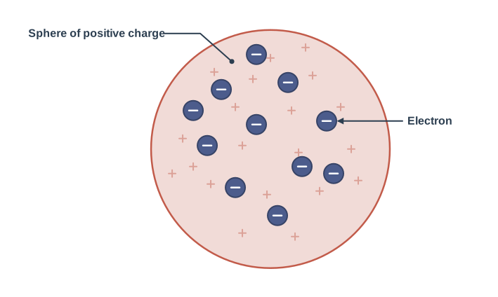
Fig. 12.1 – Thomson’s plum pudding model.

As this chapter unfolds, we will see that the real arrangement of charge inside the atom turns out to be very different from Thomson’s picture. But to understand what replaced it, we first need to see how atoms reveal their inner secrets — through the light they give out.

Light from atoms: continuous versus discrete

We know that dense matter — solids, liquids, and even dense gases — glows when heated. At every temperature such matter gives out electromagnetic radiation (energy that travels as waves, of which visible light is one part). When this radiation is separated out by wavelength, we get its spectrum. A spectrum is simply the pattern obtained when radiation is spread into its different wavelengths, the way a glass prism spreads sunlight into a band of colours.

For dense hot matter, this spectrum is continuous — it contains a smooth, unbroken spread of many wavelengths, each present with a different intensity, with no gaps in between. This radiation is produced by the constant oscillation and jostling of atoms and molecules, whose behaviour is strongly governed by the close neighbours packed tightly around each of them.

The situation is completely different for a rarefied gas — a gas at very low pressure, in which the atoms are spread far apart. When such a gas is heated in a flame, or made to glow by passing electricity through it (as in a familiar neon sign or a mercury-vapour lamp), it gives out only certain specific, separate wavelengths. Instead of a smooth band, its spectrum appears as a series of sharp bright lines separated by dark gaps, as illustrated in Fig. 12.2.

Fig. 12.2

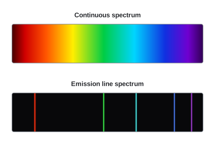
Fig. 12.2 – Continuous versus line spectrum.

Real-World Application

The coloured glow of neon advertising signs, the orange light of sodium street lamps, and the bluish light of mercury-vapour lamps all come from rarefied gases giving out their own particular set of discrete wavelengths. Each gas glows in its own characteristic colours precisely because each emits its own fixed set of bright lines.

Why the difference between the two cases? In a rarefied gas the average spacing between atoms is large, so each atom is essentially on its own, far from its neighbours. The light therefore comes from individual atoms acting independently, rather than from crowded atoms constantly interacting with one another as they do inside a solid.

The spectral fingerprint of an element

By the early nineteenth century another striking fact had been established: each element produces its own characteristic spectrum — its own fixed set of bright lines. Hydrogen, for instance, always gives the same set of lines, at the same fixed positions relative to one another, no matter where or how the hydrogen is made to glow.

This is a powerful idea. Because the pattern of lines is unique to each element, the spectrum acts like a “fingerprint” that identifies which element is present. It also hints at something deeper: the fact that the line pattern is fixed strongly suggests a close relationship between the internal structure of an atom and the light it emits. If we can decode the pattern of lines, we may be able to work out how the atom is built inside.

In 1885, Johann Jakob Balmer (1825–1898) took the first step in decoding this pattern. He found a simple empirical formula — a formula fitted to match the measurements rather than derived from any theory — that correctly gave the wavelengths of one group of lines emitted by atomic hydrogen.

Real Incident / Discovery

In 1885, Johann Jakob Balmer found a neat mathematical formula that reproduced the wavelengths of a whole group of hydrogen’s spectral lines, even though nobody yet understood why it worked. This unexplained success hinted that some hidden rule inside the atom decided exactly which wavelengths it was allowed to emit.

Because hydrogen is the simplest of all elements — a single electron around a single unit of positive charge — its spectrum is the easiest to study and to explain. For this reason we shall examine the hydrogen spectrum in detail throughout this chapter.

Towards the nuclear atom

The scientist who would finally overturn Thomson’s picture was Ernst Rutherford (1871–1937), who had earlier worked as a research student under J. J. Thomson. Rutherford was studying alpha particles — fast, positively charged particles thrown out by certain radioactive elements. In 1906 he proposed a clever idea: fire these alpha particles at atoms and study how they are scattered, using the scattering as a probe to reveal what lies hidden inside the atom.

Side Note

Ernst Rutherford (1871–1937) was a New Zealand–born British physicist who did pioneering work on radioactive radiation. He discovered alpha rays and beta rays, and together with Frederick Soddy built the modern theory of radioactivity. He studied the “emanation” of thorium and identified a new noble gas — an isotope of radon now known as thoron. By scattering alpha rays from metal foils he discovered the atomic nucleus, proposed the planetary model of the atom, and estimated the approximate size of the nucleus.

This experiment was actually carried out around 1911 by Hans Geiger (1882–1945) and Ernst Marsden (1889–1970) — Marsden being only a 20-year-old student who had not yet even earned his bachelor’s degree. The full details of the experiment are discussed in Section 12.2.

The results forced a completely new picture of the atom, known as Rutherford’s planetary model, or the nuclear model of the atom. According to this model, the entire positive charge and almost all the mass of the atom are squeezed into a very small central region called the nucleus, while the light electrons revolve around it — much as the planets revolve around the Sun (Fig. 12.3).

Definition

In Rutherford’s nuclear (planetary) model, the entire positive charge and nearly all the mass of the atom are concentrated in a tiny central nucleus, around which the electrons revolve like planets around the Sun.

Fig. 12.3

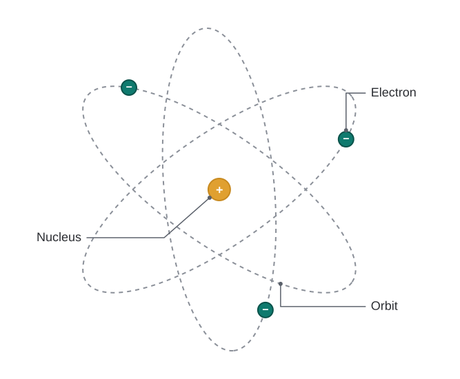
Fig. 12.3 – Rutherford’s nuclear model.

Rutherford’s nuclear model was a major step towards the modern view of the atom. Yet it could not explain one crucial fact: why do atoms emit light of only certain discrete wavelengths? How could an atom as simple as hydrogen — just one electron and one proton — produce a whole complex set of specific wavelengths?

There was an even deeper problem waiting. In the classical planetary picture, the electron revolves around the nucleus just as a planet revolves around the Sun. As we shall see, this apparently reasonable idea runs into serious difficulties that classical physics cannot resolve — difficulties that will finally push us towards the quantum ideas of Niels Bohr later in this chapter.

12.2 Alpha-particle Scattering and Rutherford’s Nuclear Model of Atom

To find out what lies inside the atom, Rutherford’s idea was simple in principle: throw something small and fast at the atom and watch how it gets deflected. The way the projectiles bounce off must depend on how charge and mass are arranged inside the target. At his suggestion, in 1911 H. Geiger and E. Marsden carried out a set of careful experiments to do exactly this.

In one of these experiments, shown in Fig. 12.4, they directed a beam of 5.5 MeV alpha particles, emitted from a \(^{214}_{83}\text{Bi}\) radioactive source, at a thin metal foil made of gold. Here MeV (mega electron volt) is simply a convenient unit of energy for tiny particles, where \(1\ \text{eV} = 1.6 \times 10^{-19}\ \text{J}\), so a 5.5 MeV alpha particle is a very fast, energetic projectile.

Fig. 12.4

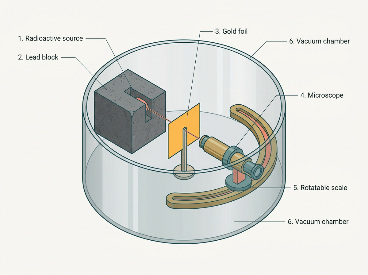
Fig. 12.4 – The Geiger–Marsden scattering apparatus.

Figure 12.5 shows the arrangement in more detail. The alpha particles from the \(^{214}_{83}\text{Bi}\) source were first collimated — narrowed into a thin, straight beam — by letting them pass through lead bricks. This narrow beam was then allowed to fall on a thin gold foil of thickness \(2.1 \times 10^{-7}\ \text{m}\).

The scattered alpha particles were picked up by a rotatable detector made of a zinc sulphide (ZnS) screen viewed through a microscope. Each alpha particle striking the screen produced a tiny flash of light called a scintillation. By counting these flashes through the microscope at different positions, the experimenters could measure how many particles were scattered at each scattering angle — the angle by which a particle is turned from its original path.

Fig. 12.5

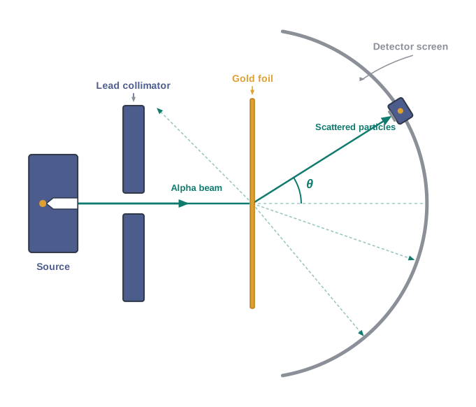
Fig. 12.5 – Schematic arrangement of the scattering experiment.

Real-World Application

The basic strategy of this experiment — fire a beam of particles at a target and study how they scatter in order to learn about the target’s inner structure — is exactly the strategy used today in giant particle accelerators and colliders. Modern physicists still probe the deepest structure of matter by scattering fast particles off it, just as Rutherford probed the atom.

What the data showed

A typical graph of the total number of alpha particles scattered at each angle, counted over a fixed time interval, is shown in Fig. 12.6. The dots are the actual measured data points, and the solid curve is the prediction of a theory built on one bold assumption: that each target atom has a small, dense, positively charged nucleus.

Fig. 12.6

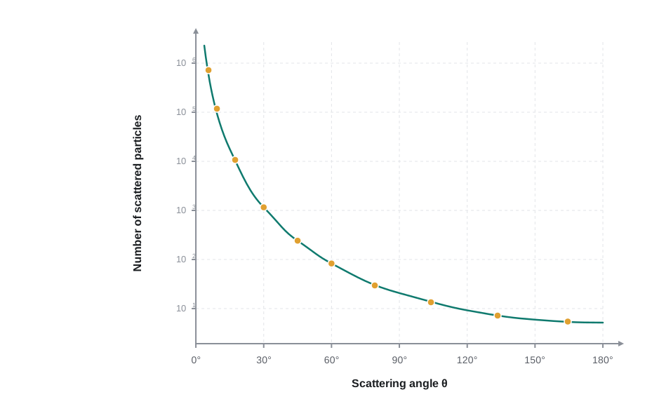
Fig. 12.6 – Scattered alpha particles versus scattering angle.

The most striking feature of the data is how few particles are deflected strongly. Most of the alpha particles pass straight through the foil, which means they suffer no collision at all. Only about 0.14% of the incident alpha particles are scattered by more than 1°, and only about 1 in 8000 are turned through more than 90°.

Rutherford reasoned as follows. To push a heavy, fast alpha particle backwards, the atom must exert a very large repulsive force on it. Such a strong force is possible only if the greater part of the atom’s mass and all of its positive charge are packed tightly into a small region at the centre. An alpha particle heading almost straight for this concentrated charge could come very close to it — without passing through it — and such a close encounter would produce a very large deflection.

The fact that the theory built on this assumption matched the data so well was strong support for the idea of a nuclear atom. This is why Rutherford is credited with the discovery of the nucleus.

Curiosity Corner

Q1. Most alpha particles passed straight through the gold foil, yet a rare few bounced almost straight back. What inside the atom could explain both of these results at once?

A. A tiny, massive, positively charged nucleus at the atom’s centre, with the rest of the atom being mostly empty space. Because the atom is largely empty, the great majority of alpha particles pass through the foil almost undeviated. But when an alpha particle happens to come very close to the minute, heavy, positively charged nucleus, the strong electrostatic repulsion turns it through a large angle — occasionally almost straight back. Both observations together point to Rutherford’s nuclear model: almost all the atom’s mass and all its positive charge are concentrated in a nucleus far smaller than the atom itself.

Principle / Law

The scattering of alpha particles by a thin gold foil shows that almost all of an atom’s mass and its entire positive charge are concentrated in a tiny central nucleus, so that the atom is mostly empty space. Most alpha particles pass through the empty space undeflected, while the rare few that approach the nucleus closely are turned through large angles.

Sizing up the atom

In Rutherford’s nuclear model, the entire positive charge and most of the mass sit in the nucleus, while the electrons move in orbits some distance away, around the nucleus, much as planets orbit the Sun. From these scattering experiments, Rutherford estimated the size of the nucleus to be about \(10^{-15}\ \text{m}\) to \(10^{-14}\ \text{m}\).

From kinetic theory, the size of a whole atom was already known to be about \(10^{-10}\ \text{m}\) — that is, roughly 10,000 to 100,000 times larger than the nucleus. So the electrons lie at a distance from the nucleus of about 10,000 to 100,000 times the size of the nucleus itself. In other words, most of an atom is empty space.

This picture immediately explains the scattering data. Because the atom is largely empty, most alpha particles sail straight through the thin foil without meeting anything. But whenever an alpha particle happens to come near a nucleus, the intense electric field there scatters it through a large angle. The atomic electrons, being extremely light, barely affect the heavy alpha particles at all.

Analysing the trajectory

The scattering data of Fig. 12.6 can be worked out quantitatively using the nuclear model. Since the gold foil is very thin, we can assume that each alpha particle is scattered by not more than one nucleus as it passes through. It is therefore enough to work out the path of a single alpha particle deflected by a single nucleus.

Alpha particles are the nuclei of helium atoms, so each carries two units of positive charge, \(2e\), and has the mass of a helium atom. The gold nucleus carries a charge \(Ze\), where \(Z\) is the atomic number of the element (the number of positive units of charge in its nucleus); for gold, \(Z = 79\).

Since the gold nucleus is about 50 times heavier than an alpha particle, we can reasonably treat it as staying still throughout the scattering. With these assumptions, the path of the alpha particle can be found using Newton’s second law of motion together with Coulomb’s law for the electrostatic force of repulsion between the alpha particle and the positively charged nucleus.

The magnitude of this repulsive Coulomb force is

\[F = \frac{1}{4\pi\varepsilon_0}\,\frac{(2e)(Ze)}{r^2} \tag{12.1}\]

where \(r\) is the distance between the alpha particle and the nucleus (in metres, m), \(2e\) is the charge of the alpha particle and \(Ze\) the charge of the nucleus (in coulombs, C), and \(\dfrac{1}{4\pi\varepsilon_0} = 9.0 \times 10^{9}\ \text{N m}^2\,\text{C}^{-2}\) is the Coulomb constant, with \(\varepsilon_0\) the permittivity of free space. The force acts along the straight line joining the alpha particle and the nucleus, and points outward because both charges are positive and repel.

As the alpha particle first approaches the nucleus and then recedes away from it, the distance \(r\) keeps changing, so both the magnitude and the direction of this force change continuously throughout the encounter. It is this changing force that bends the alpha particle’s path.

Numerical 12.1

Calculate the electrostatic force of repulsion between a gold nucleus (\(Z = 79\)) and an alpha particle when they are separated by a distance of \(5.0 \times 10^{-14}\ \text{m}\). (Take \(e = 1.6 \times 10^{-19}\ \text{C}\) and \(\dfrac{1}{4\pi\varepsilon_0} = 9.0 \times 10^{9}\ \text{N m}^2\,\text{C}^{-2}\).)

12.2.1 Alpha-particle Trajectory

We have seen that an alpha particle is deflected by the electric repulsion of a single gold nucleus. But not every alpha particle is deflected by the same amount. How sharply a given alpha particle is turned depends on how close its original path would have carried it to the nucleus. This “aim” is measured by a quantity called the impact parameter.

The impact parameter, written \(b\), is the perpendicular distance between the centre of the nucleus and the straight line along which the alpha particle is originally moving (that is, the line of its initial velocity), as shown in Fig. 12.7. A small \(b\) means the particle is aimed almost straight at the nucleus; a large \(b\) means it would pass well to one side.

Definition

The impact parameter is the perpendicular distance of the initial velocity vector of the alpha particle from the centre of the nucleus.

Fig. 12.7

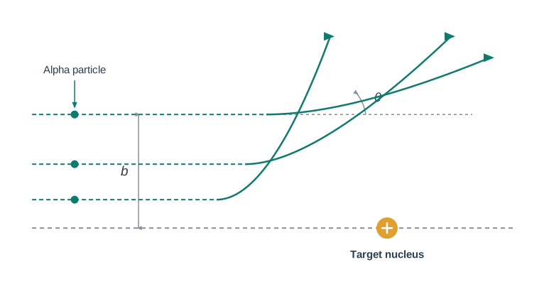
Fig. 12.7 – Alpha particle trajectories and impact parameter b.

A real beam of alpha particles contains particles with a whole range of impact parameters. Because each value of \(b\) leads to a different deflection, the beam gets scattered in many directions, each with its own probability (Fig. 12.7). Within a single beam, all the particles have nearly the same kinetic energy, so it is really the impact parameter — not the speed — that decides how much a given particle is scattered.

The pattern is clear. An alpha particle that passes close to the nucleus (small impact parameter) feels a strong repulsion and suffers large scattering. In the extreme case of a head-on collision, the impact parameter is smallest and the particle is thrown almost straight back, so the scattering angle \(\theta \cong \pi\) (about 180°). At the other extreme, for a large impact parameter the particle stays far from the nucleus, feels only a weak push, and goes almost undeviated, with \(\theta \cong 0\).

The observation that only a small fraction of the incident particles rebound backwards tells us that only a small fraction undergo near head-on collisions. This in turn confirms that the mass and positive charge of the atom are packed into a very small volume. In this way, Rutherford scattering becomes a powerful tool for setting an upper limit on the size of the nucleus.

Real-World Application

The idea of firing a charged particle at a nucleus and finding how close it can get before being turned back is still used to estimate the sizes of nuclei. By measuring the distance of closest approach for beams of different energies, physicists put limits on how small the nucleus must be.

Example 12.1

In Rutherford’s nuclear model, the nucleus (radius about \(10^{-15}\ \text{m}\)) is like the Sun, about which the electron moves in an orbit (radius \(\approx 10^{-10}\ \text{m}\)), just as the Earth orbits the Sun. If the solar system had the same proportions as the atom, would the Earth be closer to, or farther from, the Sun than it actually is? Take the radius of the Earth’s orbit as about \(1.5 \times 10^{11}\ \text{m}\) and the radius of the Sun as \(7 \times 10^{8}\ \text{m}\).

Solution The key step is to compare the two ratios. In the atom, the ratio of the radius of the electron’s orbit to the radius of the nucleus is

\[\frac{10^{-10}\ \text{m}}{10^{-15}\ \text{m}} = 10^{5},\]

so the electron’s orbit is \(10^{5}\) times larger than the nucleus.

If the Earth’s orbit around the Sun were also \(10^{5}\) times larger than the radius of the Sun, then the radius of the Earth’s orbit would be

\[10^{5} \times 7 \times 10^{8}\ \text{m} = 7 \times 10^{13}\ \text{m}.\]

This is more than 100 times greater than the Earth’s actual orbital radius. So the Earth would have to be much farther from the Sun than it really is. This tells us that an atom contains a much greater fraction of empty space than our solar system does.

Example 12.2

In a Geiger–Marsden experiment, what is the distance of closest approach to the nucleus for a 7.7 MeV alpha particle, before it comes momentarily to rest and reverses its direction?

Solution The central idea is that throughout the scattering the total mechanical energy of the alpha particle–gold nucleus system stays constant (is conserved). The initial mechanical energy \(E_i\), before the particle and nucleus interact, equals the final mechanical energy \(E_f\) at the moment the alpha particle momentarily stops.

Far away, the initial energy \(E_i\) is just the kinetic energy \(K\) of the incoming alpha particle. At the stopping point the particle is momentarily at rest, so its energy \(E_f\) is entirely the electric potential energy \(U\) of the system, which follows from Eq. (12.1). Let \(d\) be the centre-to-centre distance between the alpha particle and the gold nucleus at this stopping point. Then conservation of energy, \(E_i = E_f\), gives

\[K = \frac{1}{4\pi\varepsilon_0}\frac{(2e)(Ze)}{d} = \frac{2Ze^2}{4\pi\varepsilon_0\, d}.\]

Rearranging, the distance of closest approach \(d\) is

\[d = \frac{2Ze^2}{4\pi\varepsilon_0\, K}.\]

The maximum kinetic energy found in alpha particles of natural origin is 7.7 MeV, which is \(1.2 \times 10^{-12}\ \text{J}\). Using \(\dfrac{1}{4\pi\varepsilon_0} = 9.0 \times 10^{9}\ \text{N m}^2/\text{C}^2\) and \(e = 1.6 \times 10^{-19}\ \text{C}\),

\[d = \frac{(2)(9.0 \times 10^{9}\ \text{N m}^2/\text{C}^2)(1.6 \times 10^{-19}\ \text{C})^2\,Z}{1.2 \times 10^{-12}\ \text{J}} = 3.84 \times 10^{-16}\,Z\ \text{m}.\]

For gold, the atomic number is \(Z = 79\), so

\[d(\text{Au}) = 3.0 \times 10^{-14}\ \text{m} = 30\ \text{fm},\]

where 1 fm (one fermi) \(= 10^{-15}\ \text{m}\).

The radius of the gold nucleus must therefore be less than \(3.0 \times 10^{-14}\ \text{m}\). This does not agree very well with the observed value, since the actual radius of the gold nucleus is about 6 fm. The reason for the discrepancy is that the distance of closest approach is considerably larger than the sum of the radii of the gold nucleus and the alpha particle. In other words, the alpha particle reverses its motion without ever actually touching the gold nucleus.

Exam Corner

Q. Why does the alpha particle come to rest for an instant at the distance of closest approach?

A. As it climbs “uphill” against the repulsion of the nucleus, its kinetic energy is steadily converted into electric potential energy. At the closest point all of its kinetic energy has become potential energy, so it stops for an instant before the repulsion pushes it back out.

Numerical 12.2

A beam of 5.0 MeV alpha particles is fired head-on at silver nuclei (\(Z = 47\)). Calculate the distance of closest approach. (Take \(1\ \text{MeV} = 1.6 \times 10^{-13}\ \text{J}\), \(e = 1.6 \times 10^{-19}\ \text{C}\), and \(\dfrac{1}{4\pi\varepsilon_0} = 9.0 \times 10^{9}\ \text{N m}^2/\text{C}^2\).)

12.2.2 Electron Orbits

Rutherford’s nuclear model, which still uses ordinary (classical) ideas of mechanics, pictures the atom as an electrically neutral sphere. At its centre sits a very small, massive, positively charged nucleus, and around it move the electrons in their own steady orbits. An orbit that keeps repeating itself steadily, without the electron flying off or falling in, is called a dynamically stable orbit.

What keeps an electron moving in such a circular orbit? Any body moving in a circle must be pulled constantly towards the centre by a force called the centripetal force — without it, the body would fly off in a straight line. In the atom, this inward pull is supplied by the electrostatic force of attraction between the negatively charged electron and the positively charged nucleus.

So for a stable orbit, the electrostatic force of attraction \(F_e\) must be exactly equal to the required centripetal force \(F_c\). For the single electron in a hydrogen atom this balance gives

\[F_e = F_c\] \[\frac{1}{4\pi\varepsilon_0}\frac{e^2}{r^2} = \frac{mv^2}{r} \tag{12.2}\]

Here \(e\) is the magnitude of the charge on the electron (and on the proton) in coulombs (C), \(r\) is the orbit radius in metres (m), \(m\) is the mass of the electron in kilograms (kg), \(v\) is the electron’s speed in metres per second (m s⁻¹), and \(\dfrac{1}{4\pi\varepsilon_0} = 9.0 \times 10^{9}\ \text{N m}^2/\text{C}^2\) is the Coulomb constant. The left side is the attractive Coulomb force; the right side is the centripetal force \(mv^2/r\) needed for circular motion.

Principle / Law

For a dynamically stable electron orbit in the hydrogen atom, the electrostatic force of attraction between the electron and the nucleus provides exactly the centripetal force required to keep the electron moving in its circular path.

Rearranging Eq. (12.2) gives the relation between the orbit radius and the electron’s speed:

\[r = \frac{e^2}{4\pi\varepsilon_0\, m v^2} \tag{12.3}\]

Energy of the orbiting electron

We can now find the energy of the electron. Its kinetic energy \(K\) comes from its motion, and using Eq. (12.2) to replace \(mv^2\) we get

\[K = \frac{1}{2}mv^2 = \frac{e^2}{8\pi\varepsilon_0\, r}\]

Its electrostatic potential energy \(U\), due to the attraction of the nucleus, is

\[U = -\frac{e^2}{4\pi\varepsilon_0\, r}\]

The negative sign in \(U\) signifies that the electrostatic force is directed in the \(-r\) direction — that is, it pulls the electron inward, toward the nucleus. (By convention the potential energy is taken as zero when the electron is infinitely far away; as it is pulled closer, its potential energy falls below zero.)

Adding these, the total energy \(E\) of the electron in the hydrogen atom is

\[E = K + U = \frac{e^2}{8\pi\varepsilon_0\, r} - \frac{e^2}{4\pi\varepsilon_0\, r} = -\frac{e^2}{8\pi\varepsilon_0\, r} \tag{12.4}\]

The total energy comes out negative. This is not a mistake — it expresses the important fact that the electron is bound to the nucleus. Energy would have to be supplied from outside to pull the electron away. If instead \(E\) were positive, the electron would not follow a closed orbit around the nucleus at all; it would simply escape.

Numerical 12.3

The electron in a hydrogen atom moves in a circular orbit of radius \(5.3 \times 10^{-11}\ \text{m}\). Calculate the electrostatic force of attraction between the electron and the nucleus that provides the centripetal force. (Take \(e = 1.6 \times 10^{-19}\ \text{C}\) and \(\dfrac{1}{4\pi\varepsilon_0} = 9.0 \times 10^{9}\ \text{N m}^2/\text{C}^2\).)

Example 12.3

It is found by experiment that 13.6 eV of energy is needed to separate a hydrogen atom into a proton and an electron. Find the orbital radius and the speed of the electron in the hydrogen atom.

Solution If 13.6 eV is needed to pull the electron completely away, then the electron’s total energy in the atom must be \(-13.6\ \text{eV}\). Converting to joules,

\[E = -13.6 \times 1.6 \times 10^{-19}\ \text{J} = -2.2 \times 10^{-18}\ \text{J}.\]

From Eq. (12.4), \(E = -\dfrac{e^2}{8\pi\varepsilon_0\, r} = -2.2 \times 10^{-18}\ \text{J}\). Solving for the orbital radius,

\[r = -\frac{e^2}{8\pi\varepsilon_0\, E} = -\frac{(9 \times 10^{9}\ \text{N m}^2/\text{C}^2)(1.6 \times 10^{-19}\ \text{C})^2}{(2)(-2.2 \times 10^{-18}\ \text{J})} = 5.3 \times 10^{-11}\ \text{m}.\]

The speed of the revolving electron then follows from Eq. (12.3), using the electron mass \(m = 9.1 \times 10^{-31}\ \text{kg}\):

\[v = \frac{e}{\sqrt{4\pi\varepsilon_0\, m r}} = 2.2 \times 10^{6}\ \text{m/s}.\]

This radius, about \(5.3 \times 10^{-11}\ \text{m}\), is the size we expect for a hydrogen atom, and the electron speed of \(2.2 \times 10^{6}\ \text{m/s}\) is large but still far below the speed of light.

12.3 Atomic Spectra

As we noted in Section 12.1, every element gives out its own characteristic spectrum of radiation. We now look more closely at what these spectra look like, because they hold the clues to how the atom is built.

When an atomic gas or vapour is excited at low pressure — usually by passing an electric current through it — the light it gives out contains only certain specific wavelengths, not a continuous range. A spectrum of this kind is called an emission line spectrum, because it appears as a set of bright, sharp lines standing out against a dark background.

Definition

An emission line spectrum is the spectrum obtained when an excited atomic gas or vapour at low pressure emits light of only certain specific wavelengths, appearing as bright lines on a dark background.

The emission line spectrum of atomic hydrogen is shown in Fig. 12.8. Notice how the bright lines are not scattered at random but fall into distinct groups, or series, each labelled with a name — for hydrogen these include the Lyman, Balmer, and Paschen series. (It was one such group, the Balmer series, whose wavelengths Balmer’s 1885 formula successfully described.)

Fig. 12.8

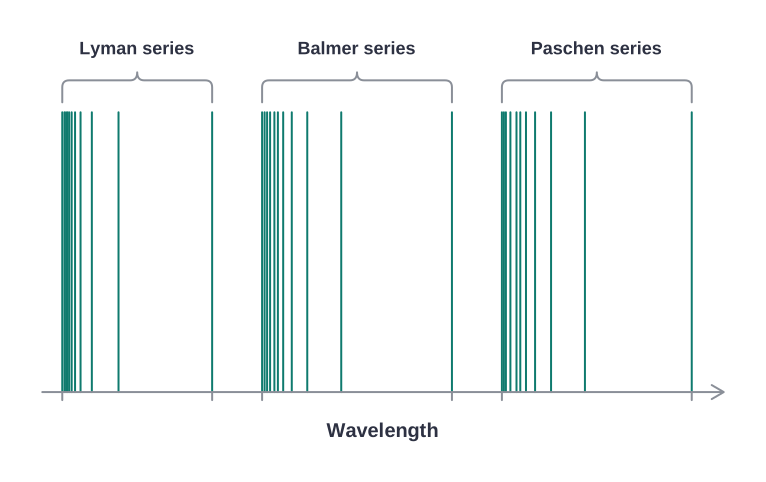
Fig. 12.8 – Emission line spectrum of atomic hydrogen.

Because each element produces its own unique pattern of bright lines, studying an emission line spectrum works like reading a “fingerprint”: from the pattern of lines alone, we can tell which element is present in a glowing gas.

Real-World Application

Astronomers use exactly this fingerprinting to work out what distant stars are made of. Even though we can never bring a sample of a star to a laboratory, the pattern of spectral lines in its light tells us which elements it contains. The same technique is used in flame tests and in identifying gases in the laboratory.

Real Incident / Discovery

The element helium was first found not on Earth but in the Sun. In 1868, during a solar eclipse, astronomers noticed a bright yellow spectral line that matched no known element. It was concluded that a new element existed in the Sun, and it was named helium after the Greek word helios, meaning Sun. Only years later was helium finally identified on Earth — a striking demonstration of the power of spectral fingerprints.

The absorption spectrum

There is a second kind of spectrum that carries the same information in reverse. Suppose we pass white light — which contains all visible wavelengths — through a gas, and then analyse the transmitted light using a spectrometer (an instrument that spreads light out by wavelength so the pattern can be examined).

When we do this, we find some dark lines cutting across the otherwise continuous spectrum. These dark lines fall exactly at the wavelengths that the same gas would emit as bright lines in its emission spectrum. This pattern of dark lines on a continuous background is called the absorption spectrum of the gas.

Definition

An absorption spectrum is the spectrum obtained when white light passes through a gas: dark lines appear at precisely those wavelengths that the gas would otherwise emit, because the gas absorbs light at exactly those wavelengths.

Fig. 12.9

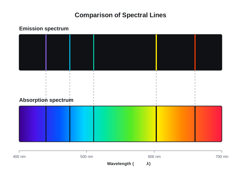
Fig. 12.9 – Emission versus absorption spectrum.

Together, the emission and absorption spectra show that each atom is fussy about wavelengths: it deals only with its own special set. Explaining why an atom is restricted to these particular wavelengths is the central task that Bohr’s model, coming up next, was built to solve.

12.4 Bohr Model of the Hydrogen Atom

Rutherford’s model treats the atom — a central nucleus with a revolving electron — as though it were as stable as the Sun–planet system it imitates. But there are some deep differences between the two cases, and these differences turn out to be fatal for the classical picture.

The first difference is the kind of force involved. A planetary system is held together by the gravitational force, whereas the nucleus and electron are charged objects that interact through Coulomb’s law. This distinction matters enormously, because a moving charge behaves very differently from a moving mass according to classical physics.

Recall that an object moving in a circle is being constantly accelerated — its centripetal acceleration always points toward the centre, even if its speed is steady. Now bring in a crucial result of classical electromagnetic theory: an accelerating charged particle must radiate energy in the form of electromagnetic waves.

If this rule held inside the atom, the orbiting electron — always accelerating — would continuously lose energy as radiation. Losing energy, it could not maintain its orbit; it would spiral steadily inward and finally crash into the nucleus, as suggested in Fig. 12.10. Such an atom could not be stable, yet atoms are obviously stable. This is the stability problem.

Fig. 12.10

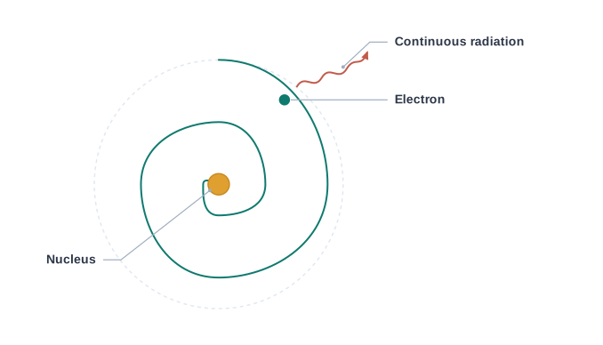
Fig. 12.10 – Classical collapse of an orbiting electron.

There is a second, related problem. Classical theory also says that the frequency of the emitted electromagnetic waves equals the electron’s frequency of revolution. As the electron spiralled inward, its speed and therefore its frequency of revolution would keep changing smoothly, so the frequency of the emitted light would also change smoothly. The atom would then radiate a continuous spectrum — flatly contradicting the sharp line spectrum that is actually observed.

Clearly, Rutherford’s model tells only part of the story. The classical ideas of mechanics and electromagnetism are simply not enough to explain the structure of the atom.

Example 12.4

Using classical electromagnetic theory, calculate the initial frequency of the light emitted by the electron revolving around a proton in a hydrogen atom.

Solution From Example 12.3, the electron moving around the proton in an orbit of radius \(5.3 \times 10^{-11}\ \text{m}\) has a speed of \(2.2 \times 10^{6}\ \text{m/s}\). The number of revolutions it makes per second — its frequency of revolution — is its speed divided by the circumference \(2\pi r\):

\[\nu = \frac{v}{2\pi r} = \frac{2.2 \times 10^{6}\ \text{m s}^{-1}}{2\pi\,(5.3 \times 10^{-11}\ \text{m})} \approx 6.6 \times 10^{15}\ \text{Hz}.\]

According to classical electromagnetic theory, the frequency of the emitted light equals this frequency of revolution. So the classical prediction for the initial frequency of the light emitted is \(6.6 \times 10^{15}\ \text{Hz}\) — a single frequency that would then change continuously as the electron spiralled in, again giving a continuous spectrum rather than sharp lines.

Bohr’s three postulates

It was Niels Bohr (1885–1962) who broke the deadlock, by adding ideas from the newly developing quantum hypothesis. Bohr had spent several months in Rutherford’s laboratory in 1912 and was convinced that the nuclear model was correct. Faced with the dilemma above, Bohr concluded in 1913 that although classical electromagnetic theory works beautifully for large-scale phenomena, it simply cannot be applied to processes at the atomic scale.

Side Note

Niels Henrik David Bohr (1885–1962) was a Danish physicist who explained the spectrum of the hydrogen atom using quantum ideas. He also gave a theory of nuclear fission based on the liquid-drop model of the nucleus. Bohr contributed greatly to clarifying conceptual problems in quantum mechanics, in particular by proposing the complementarity principle.

A radical departure from classical mechanics and electromagnetism was needed. Bohr combined classical ideas with early quantum concepts and expressed his theory as three postulates.

First postulate (stable orbits). Bohr proposed that an electron in an atom can revolve in certain special stable orbits without radiating energy — directly contradicting classical electromagnetic theory. Each atom therefore has certain definite stable states, each with a definite total energy. These are called the stationary states of the atom.

Principle / Law

Bohr’s first postulate: An electron in an atom can revolve in certain stable orbits without the emission of radiant energy. Each such state has a definite total energy and is called a stationary state.

This single bold assumption resolves the stability problem: in a stationary state the electron simply does not radiate, so it never loses energy and never spirals into the nucleus. The atom stays stable.

Curiosity Corner

Q2. If the electron simply circles the nucleus like a planet around the sun, why doesn’t it lose energy, spiral inward, and make the atom collapse in an instant?

A. Because of Bohr’s first postulate: the electron can occupy only certain special, stationary orbits, and while in one of these it does not radiate energy at all — despite being accelerated. Classical theory would have an orbiting electron continuously radiate, lose energy, and spiral into the nucleus in a fraction of a second. Bohr’s model forbids this by allowing only discrete stable orbits with no radiation; the electron loses energy only when it jumps from a higher allowed orbit to a lower one, not continuously, so the atom is stable and does not collapse.

Second postulate (quantised angular momentum). Bohr’s second postulate says which orbits are the allowed stable ones. The electron may revolve only in those orbits for which its angular momentum is a whole-number multiple of \(h/2\pi\), where \(h\) is Planck’s constant, \(h = 6.6 \times 10^{-34}\ \text{J s}\). The angular momentum \(L\) of the orbiting electron is thus quantised:

\[L = \frac{nh}{2\pi} \tag{12.5}\]

Here \(n = 1, 2, 3, \dots\) is a positive whole number called the principal quantum number, \(L\) is the angular momentum (in J s), and \(h\) is Planck’s constant. “Quantised” means the angular momentum cannot take just any value — only these special separated values are allowed.

Principle / Law

Bohr’s second postulate: The electron revolves only in those orbits for which its angular momentum is an integral multiple of \(h/2\pi\); that is, \(L = nh/2\pi\), with \(n = 1, 2, 3, \dots\)

Third postulate (transitions and photons). Bohr’s third postulate brings in the quantum ideas of Planck and Einstein. It states that an electron may jump — make a transition — from one of its stationary orbits to another of lower energy. When it does so, a photon (a discrete packet of light energy, as studied in the previous chapter) is emitted, carrying energy exactly equal to the difference in energy between the two states. If the initial and final energies are \(E_i\) and \(E_f\), the frequency \(\nu\) of the emitted photon is

\[h\nu = E_i - E_f \tag{12.6}\]

where \(E_i\) and \(E_f\) are the energies of the initial and final states (in joules, J), with \(E_i > E_f\), and \(\nu\) is the photon frequency (in hertz, Hz).

Principle / Law

Bohr’s third postulate: When an electron makes a transition from a stationary state of energy \(E_i\) to one of lower energy \(E_f\), a photon is emitted whose frequency satisfies \(h\nu = E_i - E_f\).

Fig. 12.11

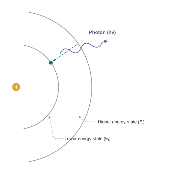
Fig. 12.11 – Photon emission during an electron transition.

Radius and energy of the allowed orbits

Bohr’s postulates let us pin down the exact radii and energies of the allowed orbits of hydrogen. Equation (12.4) already gives the total energy in terms of the orbit radius \(r\), but we still need \(r\) itself. To find it, we use the quantisation condition from the second postulate.

Writing the angular momentum as \(L = mvr\), the second postulate gives \(mvr = nh/2\pi\), so \(v = nh/(2\pi m r)\). Substituting this speed into the force-balance relation of Eq. (12.2) and solving for \(r\) gives the radius of the \(n\)th allowed orbit:

\[r_n = \left(\frac{n^2}{m}\right)\left(\frac{h}{2\pi}\right)^2 \frac{4\pi\varepsilon_0}{e^2} \tag{12.7}\]

Notice that the radius grows as \(n^2\): the allowed orbits get rapidly larger for higher \(n\).

Substituting this orbital radius back into Eq. (12.4) gives the total energy of the electron in the \(n\)th stationary state:

\[E_n = -\left(\frac{e^2}{8\pi\varepsilon_0}\right)\left(\frac{m}{n^2}\right)\left(\frac{2\pi}{h}\right)^2\left(\frac{e^2}{4\pi\varepsilon_0}\right)\]

which simplifies to

\[E_n = -\frac{m e^4}{8 n^2 \varepsilon_0^2 h^2} \tag{12.8}\]

Putting in the numerical values of the constants, this becomes

\[E_n = -\frac{2.18 \times 10^{-18}}{n^2}\ \text{J} \tag{12.9}\]

Atomic energies are often more conveniently expressed in electron volts (eV) rather than joules. Since \(1\ \text{eV} = 1.6 \times 10^{-19}\ \text{J}\), Eq. (12.9) can be rewritten as

\[E_n = -\frac{13.6}{n^2}\ \text{eV} \tag{12.10}\]

As before, the negative sign of the total energy means the electron is bound to the nucleus. Energy must be supplied from outside to remove the electron from the hydrogen atom and carry it to an infinite distance from the nucleus (the proton).

Numerical 12.4

Using Bohr’s second postulate, calculate the angular momentum of the electron in the \(n = 4\) orbit of a hydrogen atom. (Take \(h = 6.6 \times 10^{-34}\ \text{J s}\).)

12.4.1 Energy Levels

Equation (12.10), \(E_n = -13.6/n^2\) eV, tells us that the electron in a hydrogen atom can have only certain fixed energies, one for each value of \(n\). It is worth looking closely at what these allowed energies mean.

The energy of the atom is least — that is, has the largest negative value — when the electron is in the orbit closest to the nucleus, the one with \(n = 1\). As \(n\) increases to \(2, 3, \dots\), the absolute value of the energy becomes smaller, so the energy itself becomes progressively larger (less negative) for the outer orbits.

The lowest-energy state of all, with \(n = 1\), is called the ground state. In it, the electron revolves in the orbit of smallest radius, called the Bohr radius, written \(a_0\). The energy of this state is \(E_1 = -13.6\ \text{eV}\).

Definition

The ground state of an atom is its lowest-energy state, in which the electron occupies the orbit of smallest radius (the Bohr radius). For hydrogen, the ground-state energy is \(E_1 = -13.6\ \text{eV}\).

Because the ground-state energy is \(-13.6\ \text{eV}\), the minimum energy needed to remove the electron completely from the ground state — to pull it infinitely far away — is \(13.6\ \text{eV}\). This is called the ionisation energy of the hydrogen atom. Remarkably, this predicted value agrees excellently with the experimentally measured ionisation energy of hydrogen, a major success for Bohr’s model.

Definition

The ionisation energy of an atom is the minimum energy required to remove its electron completely from the ground state to an infinite distance. For hydrogen it is \(13.6\ \text{eV}\).

Excitation and the excited states

At room temperature, most hydrogen atoms sit quietly in the ground state. But if a hydrogen atom receives energy — for example, through collisions with fast-moving electrons — it may gain enough energy to lift its electron into one of the higher-energy orbits. The atom is then said to be in an excited state.

Definition

An excited state is any allowed state of the atom with energy higher than the ground state (\(n > 1\)), reached when the atom absorbs energy that lifts its electron to a higher orbit.

We can work out exactly how much energy is needed. From Eq. (12.10), for \(n = 2\) the energy is \(E_2 = -3.40\ \text{eV}\). So to raise the electron to this first excited state requires \[E_2 - E_1 = -3.40\ \text{eV} - (-13.6\ \text{eV}) = 10.2\ \text{eV}.\]

Similarly, \(E_3 = -1.51\ \text{eV}\), so to excite the atom from its ground state (\(n = 1\)) to the second excited state (\(n = 3\)) requires \[E_3 - E_1 = 12.09\ \text{eV},\] and so on for higher levels.

Once in an excited state, the electron can fall back to a lower-energy state, and in doing so it emits a photon (this is exactly the process described by Bohr’s third postulate). One further point is worth noting: as the excitation increases — that is, as \(n\) increases — the extra energy still needed to free the electron from that excited atom becomes smaller and smaller.

Real-World Application

The shimmering light of the aurora (the Northern and Southern Lights) is this very process on a grand scale. High-energy particles from the Sun collide with oxygen and nitrogen atoms high in the atmosphere, exciting their electrons to higher energy states. As these electrons fall back down, the atoms emit photons — the greenish and reddish glow we see in the polar sky.

The energy level diagram

All of this information is captured neatly in an energy level diagram for hydrogen, computed from Eq. (12.10) and shown in Fig. 12.12. Each horizontal line represents one allowed energy, and the principal quantum number \(n\) labels the states in increasing order of energy.

Fig. 12.12

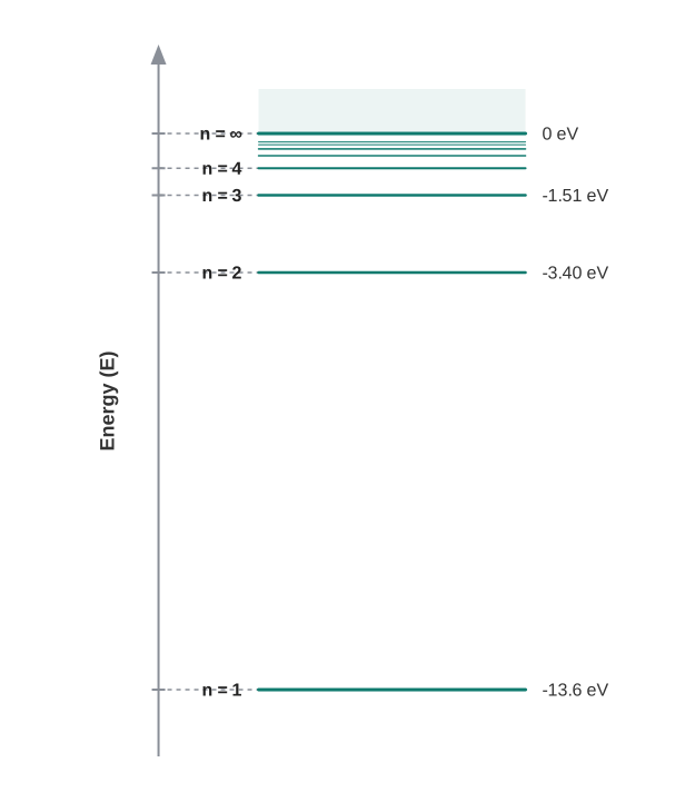
Fig. 12.12 – Energy level diagram of the hydrogen atom.

In this diagram the highest state corresponds to \(n = \infty\) in Eq. (12.10) and has an energy of exactly \(0\ \text{eV}\). This is the energy of the atom when the electron has been completely removed (\(r = \infty\)) and is at rest. An important feature to observe is how the energy levels of the excited states crowd closer and closer together as \(n\) increases.

An electron can also have any total energy above \(0\ \text{eV}\). In that case it is no longer bound to the nucleus at all — it is free. So above \(E = 0\ \text{eV}\) there is a continuous range (a continuum) of allowed energies, rather than separated levels.

Numerical 12.5

How much energy must a hydrogen atom absorb to raise its electron from the first excited state (\(n = 2\)) to the level \(n = 4\)? (Use \(E_n = -13.6/n^2\) eV.)

12.5 The Line Spectra of the Hydrogen Atom

We now have everything needed to explain the puzzle we started with: why hydrogen emits only certain sharp lines rather than a continuous rainbow. The answer follows directly from Bohr’s third postulate combined with the discrete energy levels of Section 12.4.1.

Suppose the atom makes a transition from a higher energy state, labelled by the quantum number \(n_i\), to a lower one labelled \(n_f\) (with \(n_f < n_i\)). The energy difference is carried away by a single photon whose frequency \(\nu_{if}\) satisfies

\[h\nu_{if} = E_{n_i} - E_{n_f} \tag{12.11}\]

Here \(E_{n_i}\) and \(E_{n_f}\) are the energies of the initial and final states (in joules, J), \(h\) is Planck’s constant, and \(\nu_{if}\) is the frequency of the emitted photon (in hertz, Hz).

Now comes the crucial point. Since \(n_i\) and \(n_f\) can only be whole numbers, the energies \(E_{n_i}\) and \(E_{n_f}\) can only take the discrete values fixed by Eq. (12.10). Therefore their difference, and hence the photon frequency, can only take certain discrete values as well. In other words, light is radiated only at a set of separate, specific frequencies — exactly the sharp bright lines observed in the spectrum, and never a continuous band.

Curiosity Corner

Q3. Why does hydrogen gas glow with only a few specific colours of light instead of a smooth, continuous rainbow?

A. Because the electron in a hydrogen atom can have only certain discrete (quantised) energies, one for each allowed orbit. Light is emitted when the electron jumps from a higher energy level to a lower one, and the emitted photon carries exactly the energy difference between the two levels, \(h\nu = E_i - E_f\). Since only particular energy differences are possible, only particular photon energies — and hence only particular colours (wavelengths) — are emitted. This gives a spectrum of a few sharp bright lines rather than a continuous rainbow.

Principle / Law

The line spectrum of hydrogen arises because the atom’s energy levels are discrete. A photon is emitted only when the electron jumps between two of these levels, and since only certain level differences are possible, only certain discrete frequencies (spectral lines) appear.

Emission and absorption lines

The bright lines of the spectrum are produced when electrons jump down from a higher energy state to a lower one, releasing photons. These are called emission lines.

The reverse can also happen. If an atom is struck by a photon whose energy is precisely the amount needed to lift its electron from a lower level to a higher one, the atom absorbs that photon and the electron jumps up. This is called absorption.

So if light containing a continuous range of frequencies is passed through a rarefied gas and then analysed, a series of dark lines appears in the otherwise continuous spectrum — the absorption spectrum introduced in Section 12.3. Each dark line marks a frequency that has been removed from the beam by the atoms of the gas.

Patterns in the spectrum: the spectral series

The allowed lines are not random. They fall into distinct groups, or series, according to which level the electron finally lands on. Transitions that end on the ground state (\(n_f = 1\)) form the Lyman series; those ending on \(n_f = 2\) form the Balmer series; those ending on \(n_f = 3\) form the Paschen series, and so on. This is why the hydrogen spectrum of Fig. 12.8 shows its lines organised into neat groups rather than scattered at random.

Fig. 12.13

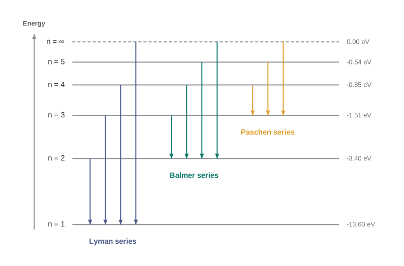
Fig. 12.13 – Spectral series transitions in hydrogen.

So there is indeed a definite rule behind which wavelengths hydrogen can emit or absorb: they are precisely the wavelengths corresponding, through Eq. (12.11), to jumps between the discrete energy levels of the atom.

Curiosity Corner

Q4. Is there a rule or pattern that decides exactly which wavelengths a hydrogen atom can emit or absorb?

A. Yes. Each wavelength comes from a transition between two allowed levels of energy \(E_n = -13.6/n^2\) eV, and the emitted or absorbed photon satisfies \(h\nu = E_{n_i} - E_{n_f}\). Grouping the transitions by the level they end on (or start from) produces the observed spectral series — for hydrogen these are the Lyman, Balmer, Paschen and other series — and the wavelengths within them follow a regular formula. So the permitted wavelengths are not random: they are fixed by the quantised energy levels and the transitions allowed between them.

Real-World Application

Because hydrogen’s spectral lines occur at exactly known frequencies, astronomers use them as fixed reference marks. When these lines from a distant galaxy appear shifted toward longer wavelengths (a redshift), the amount of shift reveals how fast the galaxy is moving away — evidence that our Universe is expanding.

The explanation of the hydrogen spectrum was a brilliant achievement of Bohr’s model and gave a huge push to the development of modern quantum theory. In recognition of this work, Niels Bohr was awarded the Nobel Prize in Physics in 1922.

Numerical 12.6

Calculate the wavelength of the photon emitted when the electron in a hydrogen atom falls from the \(n = 3\) level to the \(n = 2\) level. (Use \(E_n = -13.6/n^2\) eV, \(1\ \text{eV} = 1.6 \times 10^{-19}\ \text{J}\), \(h = 6.6 \times 10^{-34}\ \text{J s}\), and \(c = 3 \times 10^{8}\ \text{m/s}\).)

12.6 De Broglie’s Explanation of Bohr’s Second Postulate of Quantisation

Bohr’s model works beautifully, but one of its postulates was left hanging as a bare assumption. Of all his ideas, the most puzzling is the second postulate: that the angular momentum of the orbiting electron can only be a whole-number multiple of \(h/2\pi\), that is, \(L_n = nh/2\pi\) with \(n = 1, 2, 3, \dots\). Bohr simply assumed this. But why should angular momentum be restricted to exactly these values, and not any others?

The French physicist Louis de Broglie answered this puzzle in 1923, ten years after Bohr proposed his model — and his answer came from the wave nature of the electron.

In the previous chapter (Chapter 11) we met de Broglie’s hypothesis that material particles, such as electrons, also behave like waves, with a wavelength \(\lambda = h/p\), where \(p\) is the particle’s momentum. This was no mere guess: C. J. Davisson and L. H. Germer later confirmed the wave nature of electrons experimentally in 1927.

Real Incident / Discovery

In 1927, Davisson and Germer fired a beam of electrons at a crystal and found that the electrons were diffracted — bending and reinforcing in a pattern just like waves passing through a grating. This was direct experimental proof that electrons really do behave as waves, exactly as de Broglie had proposed.

Real-World Application

The wave nature of electrons is the working principle of the electron microscope. Because fast electrons have a far shorter wavelength than visible light, an electron microscope can resolve much finer detail than any light microscope, revealing structures far too small to see with ordinary light.

The standing-wave picture

De Broglie argued that the electron in its Bohr orbit should be pictured not as a tiny ball but as a particle wave wrapped around the orbit. And just as waves on a string can settle into steady standing waves under the right (resonant) conditions, so too can the electron’s particle wave.

Recall from Class XI Physics (Chapter 14) what happens when a string is plucked: a huge number of wavelengths are set off, but only certain ones survive. The surviving waves are those that have nodes (points of no motion) at the fixed ends and form a steady standing wave. In terms of distance, a standing wave forms only when the total distance a wave travels down the string and back is a whole number of wavelengths — one, two, three, and so on. Waves of any other wavelength interfere destructively with themselves after reflection, and their amplitude quickly dies away to zero.

Now apply the same idea to the electron. For an electron going around the \(n\)th circular orbit of radius \(r_n\), the “loop” it must fit into is the circumference of the orbit, \(2\pi r_n\). For its wave to survive as a steady standing wave, this circumference must contain a whole number of wavelengths:

\[2\pi r_n = n\lambda, \qquad n = 1, 2, 3, \dots \tag{12.12}\]

Principle / Law

An electron can occupy only those orbits whose circumference contains a whole number of de Broglie wavelengths: \(2\pi r_n = n\lambda\). Only such orbits support a stable standing wave; all others cancel out.

Figure 12.14 shows this standing particle wave for the case \(n = 4\), where exactly four de Broglie wavelengths fit around the orbit, so that \(2\pi r_n = 4\lambda\).

Fig. 12.14

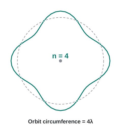
Fig. 12.14 – Standing de Broglie wave for n = 4.

Curiosity Corner

Q5. Why is an electron allowed to sit only in certain special orbits inside the atom, and not at just any distance from the nucleus?

A. Because of the wave nature of the electron. De Broglie’s picture treats the orbiting electron as a wave, and only orbits whose circumference holds a whole number of electron wavelengths (\(2\pi r = n\lambda\)) allow the wave to close on itself and form a stable standing wave; other orbits would have the wave interfere destructively and cancel out. This standing-wave condition is exactly Bohr’s second postulate, that the angular momentum is quantised as \(mvr = nh/2\pi\). So only certain special radii give self-consistent standing waves, and these are the allowed orbits.

Recovering Bohr’s second postulate

We can now turn Eq. (12.12) into Bohr’s quantisation rule. From Chapter 11, the electron’s de Broglie wavelength is \(\lambda = h/p\). As long as the electron’s speed is much less than the speed of light, its momentum is simply \(p = mv_n\), so \(\lambda = h/mv_n\). Substituting this into Eq. (12.12):

\[2\pi r_n = \frac{nh}{mv_n} \qquad \text{or} \qquad m v_n r_n = \frac{nh}{2\pi}\]

But \(mv_n r_n\) is exactly the angular momentum of the electron. So we have arrived at \(L = nh/2\pi\) — precisely the quantum condition Bohr had assumed in his second postulate, Eq. (12.5). As we saw earlier in the chapter, this same condition is what fixes the discrete orbits and energy levels of hydrogen.

De Broglie’s hypothesis thus explained Bohr’s second postulate rather than merely assuming it: the quantised orbits and energy states exist because the electron is a wave, and only resonant standing waves can persist around the nucleus.

Numerical 12.7

In the ground state (\(n = 1\)) of hydrogen, the electron moves with speed \(2.2 \times 10^{6}\ \text{m/s}\) in an orbit of radius \(5.3 \times 10^{-11}\ \text{m}\). Calculate the electron’s de Broglie wavelength and verify that it equals the circumference of the orbit. (Take \(h = 6.6 \times 10^{-34}\ \text{J s}\), \(m = 9.1 \times 10^{-31}\ \text{kg}\).)

Limitations of Bohr’s model

Bohr’s model, with its classical picture of a planet-like electron circling the nucleus, correctly predicts the gross features of hydrogenic atoms — in particular, the frequencies of the light they emit or selectively absorb. Yet the model has serious limitations. Two important ones are the following.

(i) It works only for single-electron (hydrogenic) atoms. The model cannot be extended even to a two-electron atom such as helium. Attempts to analyse multi-electron atoms along Bohr’s lines simply failed. The reason is that in such atoms each electron interacts not only with the positively charged nucleus but also with every other electron. Bohr’s model includes only the electrical force between the nucleus and one electron; it leaves out the electron–electron forces that must appear in multi-electron atoms.

(ii) It cannot explain the relative intensities of the spectral lines. Although Bohr’s model correctly predicts the frequencies of the light emitted by hydrogenic atoms, it cannot say why some lines are bright and others faint. In the emission spectrum of hydrogen, some frequencies come out strong and others weak, because experiment shows that certain transitions are more favoured than others. Bohr’s model offers no way to account for these intensity differences.

Definition

Hydrogenic atoms are atoms consisting of a nucleus with positive charge \(+Ze\) and a single electron, where \(Z\) is the proton number. Examples include the hydrogen atom, singly ionised helium, and doubly ionised lithium — atoms in which electron–electron interactions do not arise.

For all its elegance, then, Bohr’s model presents only a partial picture of the atom, and it cannot be generalised to complex atoms. To describe those, physicists had to develop a new and more radical theory — quantum mechanics — which provides a far more complete picture of atomic structure. But Bohr’s model remains a landmark: it was the first successful step in showing that the atom is governed by quantum rules.

12.7 Summary

An atom as a whole is electrically neutral, so it contains equal amounts of positive and negative charge.
In Thomson’s model, an atom is a spherical cloud of positive charge with the electrons embedded in it.
In Rutherford’s model, most of the mass of the atom and all of its positive charge are concentrated in a tiny nucleus (typically about one ten-thousandth the size of the atom), and the electrons revolve around it.
Rutherford’s nuclear model has two main difficulties in explaining atomic structure:
1. It predicts that atoms are unstable, because an accelerated electron revolving around the nucleus must radiate energy and spiral into the nucleus. This contradicts the observed stability of matter.
2. It cannot explain the characteristic line spectra of atoms of different elements.
Atoms of most elements are stable and emit a characteristic spectrum. This spectrum consists of a set of isolated, sharp lines called a line spectrum, and it provides useful information about atomic structure.
To explain both the line spectra and the stability of atoms, Niels Bohr proposed a model for hydrogenic (single-electron) atoms. He introduced three postulates that laid the foundations of quantum mechanics:
1. In a hydrogen atom, the electron revolves in certain stable orbits (called stationary orbits) without emitting radiant energy.
2. The stationary orbits are those for which the angular momentum is an integral multiple of \(h/2\pi\) (Bohr’s quantisation condition). That is, \(L = nh/2\pi\), where \(n\) is an integer called the principal quantum number.
3. An electron may make a transition from one of its non-radiating orbits to another of lower energy. When it does so, a photon is emitted whose energy equals the difference between the initial and final energies. The frequency \(\nu\) of the emitted photon is \[h\nu = E_i - E_f\] An atom absorbs radiation of the same frequency it can emit, in which case the electron is raised to an orbit of higher \(n\): \[E_i + h\nu = E_f\]
Because the angular momentum is quantised, the electron can orbit the nucleus only at certain specific radii. For a hydrogen atom, \[r_n = \left(\frac{n^2}{m}\right)\left(\frac{h}{2\pi}\right)^2 \frac{4\pi\varepsilon_0}{e^2}\] The total energy is also quantised: \[E_n = -\frac{m e^4}{8 n^2 \varepsilon_0^2 h^2} = -\frac{13.6}{n^2}\ \text{eV}\] The \(n = 1\) state is the ground state, with energy \(-13.6\ \text{eV}\) for hydrogen. Higher values of \(n\) correspond to excited states (\(n > 1\)). Atoms are raised to these higher states by collisions with other atoms or electrons, or by absorbing a photon of the right frequency.
De Broglie’s hypothesis that electrons have a wavelength \(\lambda = h/mv\) explained Bohr’s quantised orbits through wave–particle duality. The allowed orbits correspond to circular standing waves in which the circumference of the orbit equals a whole number of wavelengths.
Bohr’s model applies only to hydrogenic (single-electron) atoms. It cannot be extended even to two-electron atoms such as helium, and it is also unable to explain the relative intensities of the frequencies emitted, even for hydrogenic atoms.

12.8 Points to Ponder

Both Thomson’s model and Rutherford’s model describe systems that are actually unstable. Thomson’s model is unstable in an electrostatic sense, while Rutherford’s model is unstable because the orbiting electrons must lose energy through electromagnetic radiation.
Why did Bohr choose to quantise the angular momentum (in his second postulate), rather than some other quantity? There is a natural reason: Planck’s constant \(h\) has the same dimensions as angular momentum, and for circular orbits angular momentum is a very relevant quantity. Seen this way, the second postulate feels quite natural.
The neat orbital picture of Bohr’s model is inconsistent with the uncertainty principle, which forbids us from knowing an electron’s exact path. Bohr’s model was later replaced by modern quantum mechanics, in which Bohr’s sharp orbits become regions where the electron is merely most likely to be found.
In the solar system, the gravitational pull between one planet and another is tiny compared with the Sun’s pull on each planet, because the Sun is so much more massive than any planet. Inside an atom the situation is very different: the electron–electron electric force is comparable in size to the electron–nucleus force, because the charges and the distances involved are all of the same order of magnitude. This is exactly why Bohr’s planet-like model fails for many-electron atoms.
Bohr founded quantum theory by postulating special orbits in which electrons do not radiate, but his model uses only a single quantum number, \(n\). Modern quantum mechanics supports the spirit of Bohr’s postulate, yet it goes further: a single energy level need not correspond to just one quantum state. A state is in fact described by four quantum numbers (\(n\), \(l\), \(m\), and \(s\)), although for the pure Coulomb potential of the hydrogen atom the energy happens to depend only on \(n\).
In Bohr’s model — contrary to what classical physics would expect — the electron’s frequency of revolution in its orbit is not the same as the frequency of the spectral line it produces. The spectral-line frequency is instead the difference between two orbital energies divided by \(h\). Only for transitions between very large quantum numbers (from \(n\) to \(n-1\), with \(n\) very large) do the two frequencies come to coincide, as classical physics would predict.
Bohr’s model is semiclassical — part classical physics, part modern physics — and so it does not give the fully correct picture even of the simplest hydrogenic atoms. The true picture is quantum mechanical and differs from Bohr’s model in several fundamental ways. If Bohr’s model is not strictly correct, why study it at all? It remains valuable for these reasons:
1. It rests on just three postulates yet accounts for almost all the general features of the hydrogen spectrum.
2. It builds on many familiar concepts from classical physics.
3. It shows how a theoretical physicist may sometimes have to deliberately set aside certain difficulties in order to make useful predictions. If those predictions then agree with experiment, the theorist must later find a way to explain or rationalise the problems that were set aside.

12.9 NCERT Questions

Choose the correct alternative from the clues given at the end of each statement:
1. The size of the atom in Thomson’s model is ………. the atomic size in Rutherford’s model. (much greater than / no different from / much less than.)
2. In the ground state of ………. electrons are in stable equilibrium, while in ………. electrons always experience a net force. (Thomson’s model / Rutherford’s model.)
3. A classical atom based on ………. is doomed to collapse. (Thomson’s model / Rutherford’s model.)
4. An atom has a nearly continuous mass distribution in a ………. but has a highly non-uniform mass distribution in ………. (Thomson’s model / Rutherford’s model.)
5. The positively charged part of the atom possesses most of the mass in ………. (Rutherford’s model / both the models.)
Suppose you are given a chance to repeat the alpha-particle scattering experiment using a thin sheet of solid hydrogen in place of the gold foil. (Hydrogen is a solid at temperatures below 14 K.) What results do you expect?
A difference of 2.3 eV separates two energy levels in an atom. What is the frequency of radiation emitted when the atom makes a transition from the upper level to the lower level?
The ground state energy of hydrogen atom is –13.6 eV. What are the kinetic and potential energies of the electron in this state?
A hydrogen atom initially in the ground level absorbs a photon, which excites it to the \(n = 4\) level. Determine the wavelength and frequency of photon.
1. Using the Bohr’s model calculate the speed of the electron in a hydrogen atom in the \(n = 1\), 2, and 3 levels. (b) Calculate the orbital period in each of these levels.
The radius of the innermost electron orbit of a hydrogen atom is \(5.3 \times 10^{-11}\) m. What are the radii of the \(n = 2\) and \(n = 3\) orbits?
A 12.5 eV electron beam is used to bombard gaseous hydrogen at room temperature. What series of wavelengths will be emitted?
In accordance with the Bohr’s model, find the quantum number that characterises the earth’s revolution around the sun in an orbit of radius \(1.5 \times 10^{11}\) m with orbital speed \(3 \times 10^{4}\) m/s. (Mass of earth \(= 6.0 \times 10^{24}\) kg.)

Where required, use \(E_n = -\dfrac{13.6}{n^2}\) eV, \(h = 6.6 \times 10^{-34}\) J s, \(c = 3 \times 10^{8}\) m/s, \(1\ \text{eV} = 1.6 \times 10^{-19}\) J, \(e = 1.6 \times 10^{-19}\) C, and \(\dfrac{1}{4\pi\varepsilon_0} = 9.0 \times 10^{9}\) N m\(^2\)/C\(^2\).

12.10 Check Your Concepts

In the alpha-particle scattering experiment, most of the particles pass through the gold foil almost undeviated, while a very small number are turned through large angles. State what each of these two observations separately reveals about the structure of the atom.
The total energy of the electron in a hydrogen atom is negative. Explain the physical significance of this negative sign, and state what a positive total energy would imply for the electron.
Classical electromagnetic theory predicts that an orbiting electron must continuously radiate energy and spiral into the nucleus. Name the postulate of Bohr’s model that removes this difficulty, and explain how it does so.
The bright lines in the emission spectrum of a gas and the dark lines in its absorption spectrum appear at exactly the same wavelengths. Give the reason for this.
Bohr’s model successfully explains the hydrogen atom but fails even for the helium atom. Explain why.
Using the relation \(E_n = -13.6/n^2\) eV, explain why the energy levels of the hydrogen atom crowd closer and closer together as \(n\) increases.
Explain why the distance of closest approach measured in an alpha-scattering experiment gives only an upper limit to the size of the nucleus, and not its exact size.

12.11 Practice with Numericals

Calculate the wavelength of the radiation emitted when the electron in a hydrogen atom makes a transition from the \(n = 4\) level to the \(n = 2\) level.
How much energy is required to ionise a hydrogen atom that is already in its first excited state (\(n = 2\))?
Calculate the frequency of the photon emitted when the electron in a hydrogen atom falls from the \(n = 2\) level to the ground state (\(n = 1\)).
The total energy of the electron in a certain orbit of a hydrogen atom is \(-0.85\) eV. Identify the principal quantum number \(n\) of this orbit, and find the energy required to free the electron completely from this orbit.
For a hydrogen atom, find the ratio of the radius of the \(n = 3\) orbit to that of the \(n = 1\) orbit, and the ratio of the total energy in the \(n = 3\) state to that in the \(n = 1\) state.