Chapter 2: Electrostatic Potential and Capacitance
Around the year 1800, an Italian physicist named Alessandro Volta ended one of the most famous scientific arguments of his time. His countryman Luigi Galvani had noticed that a dead frog’s leg twitched when touched by two different metals, and Galvani believed he had discovered a special “animal electricity” stored inside living tissue. Volta disagreed. Through careful experiments, he showed that the electricity did not come from the frog at all — it appeared whenever any moist material was pressed between two different metals.
To prove his point, Volta built something remarkable: a tall stack of alternating metal discs, each pair separated by a piece of cardboard soaked in salt water. When he connected the top and bottom of this pile with a wire, a steady electric current flowed. He had built the world’s first battery, the “voltaic pile.”
For the first time, humans could produce a continuous, controllable push of electric charge instead of relying on brief sparks. That “push” — the difference that makes charge flow from one place to another — is exactly what this chapter is about. Volta’s name lives on in the unit we still use today: the volt.
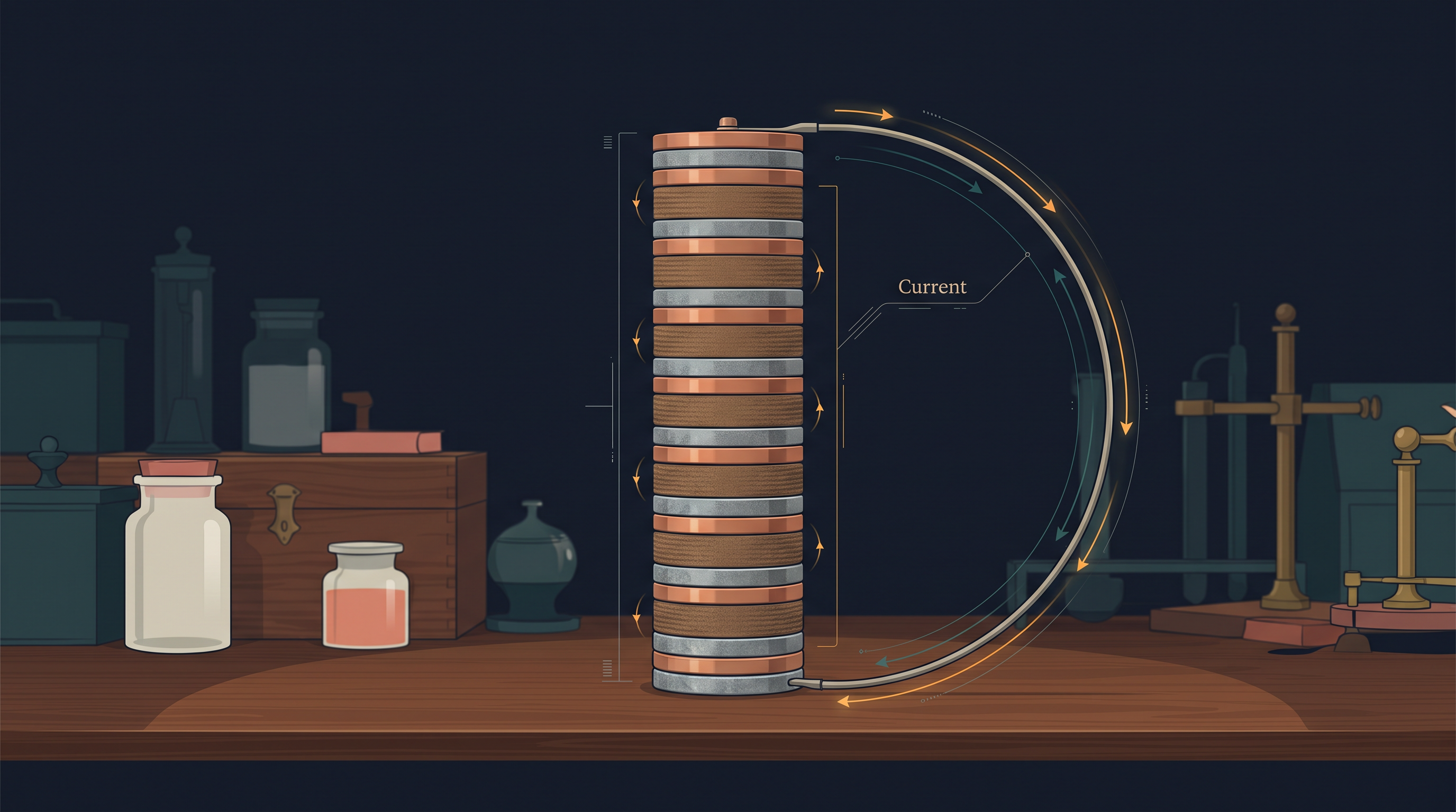
Fig. 2.0 – Volta’s voltaic pile generating a continuous electric current.
By the end of this chapter, you will be able to answer each of these questions using the ideas of electric potential, potential energy, and capacitance.
2.1 Introduction
In Classes XI you studied the idea of potential energy while learning about the spring force and the gravitational force. Potential energy is simply energy that a body stores because of its position or configuration. When you push a body slowly against a force — for example, lifting a book upward against gravity, or compressing a spring — your external push does work on the body, and that work does not vanish. It gets stored in the body as potential energy.
The stored energy can later be recovered. If you remove your external push, the body moves back: it speeds up, gaining kinetic energy (energy of motion), while losing exactly the same amount of potential energy. The total of kinetic and potential energy stays fixed throughout. In other words, the energy is conserved.
Forces that behave this way — that let work be stored and fully recovered as motion — are called conservative forces. The spring force and the gravitational force are the two familiar examples you have already met.
The Coulomb force between two stationary charges is also a conservative force. This should not surprise us. Coulomb’s law and Newton’s law of gravitation have the same mathematical shape: both fall off as the inverse square of the distance, and they differ mainly in the proportionality constant — where gravitation uses masses, Coulomb’s law uses charges. Because the two force laws are so similar in form, we can carry over the whole idea of potential energy. Just as a mass has gravitational potential energy in a gravitational field, a charge has electrostatic potential energy in an electrostatic field.
Setting up the situation
Let us make this concrete. Suppose some fixed arrangement of charges sets up an electric field \(\\vec{E}\) in the surrounding space. Recall from the previous chapter that the electric field at a point is the force experienced per unit positive charge placed there. For simplicity, take the field \(\\vec{E}\) produced by a single charge \(Q\) sitting at the origin.
Now imagine we bring a small test charge \(q\) from a point R to a point P. A test charge is simply a charge we use to probe the field. If \(Q\) and \(q\) have the same sign, they repel, so moving \(q\) closer means pushing it against the repulsive electric force, as shown in Fig. 2.1. To keep the discussion definite, let us take both \(Q\) and \(q\) to be positive.
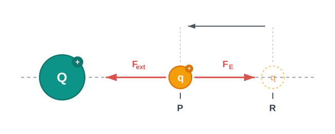
Fig. 2.1 – Work done moving a test charge against repulsion.
Two careful assumptions are worth stating clearly.
First, we take the test charge \(q\) to be so small that it does not disturb the original arrangement — it does not push the charge \(Q\) out of place. (If you like, imagine \(Q\) is held firmly at the origin by some unstated force.)
Second, while moving \(q\) from R to P, we apply an external force \(\\vec{F}\_{ext}\) that is just enough to exactly balance the repulsive electric force \(\\vec{F}*E\) on the charge. That is, \(\\vec{F}*{ext} = -\\vec{F}\_E\). Because these two forces cancel, there is no net force on \(q\) and hence no acceleration. The charge drifts from R to P infinitesimally slowly, at a steady speed.
Under this arrangement, the work done by the external force is exactly the negative of the work done by the electric force, and it is fully stored as the potential energy of the charge \(q\). If we now release the charge at P by removing the external force, the electric force pushes \(q\) back away from \(Q\): the stored potential energy is converted into kinetic energy, and once again the sum of kinetic and potential energy is conserved.
Work done and potential energy difference
The work done by the external force in moving the charge \(q\) from R to P is written as an integral of force along the path:
\[W\_{RP} = \\int\_R^P \\vec{F}\_{ext} \\cdot d\\vec{r} = -\\int\_R^P \\vec{F}\_E \\cdot d\\vec{r} \\tag{2.1}\]
Here \(\\vec{F}\_{ext}\) is the external force, \(\\vec{F}\_E\) is the electric force on the charge, and \(d\\vec{r}\) is a tiny displacement along the path; the dot product picks out the part of the force along the motion. The work is measured in joules (J). The minus sign in the second form simply reflects that the external force is opposite to the electric force. This work is done against the electric repulsion and gets stored as potential energy.
At every point in an electric field, a charge \(q\) possesses a definite electrostatic potential energy. The work \(W\_{RP}\) we just calculated is exactly the increase in that potential energy in going from R to P. So the change in potential energy equals this work:
\[\\Delta U = U\_P - U\_R = W\_{RP} \\tag{2.2}\]
where \(U\_P\) and \(U\_R\) are the potential energies of the charge at P and R. (Note that since the charge is being moved opposite to the electric force, the work done by the electric field itself is negative, i.e. \(-W\_{RP}\).)
This gives us a clean, general definition.
Two important observations
(i) The work depends only on the endpoints, not the path. The right-hand side of Eq. (2.2) involves only the starting point R and the finishing point P. This means the work done by an electrostatic field in moving a charge depends solely on the initial and final positions, and not on the particular route taken between them. This path-independence is the defining hallmark of a conservative force — indeed, the very idea of a potential energy would be meaningless if the work depended on the path chosen. (This path-independence can be proved directly from Coulomb’s law; we shall not do so here.)
(ii) Potential energy is fixed only up to a constant. Equation (2.2) defines a difference in potential energy in terms of the measurable quantity, work. This means the actual value of potential energy at a point is not, by itself, physically meaningful — only differences are. We are always free to add the same arbitrary constant \(\\alpha\) to the potential energy at every point, because it cancels out in any difference:
\[(U\_P + \\alpha) - (U\_R + \\alpha) = U\_P - U\_R\]
Put another way, we have complete freedom in choosing where the potential energy is taken to be zero.
A very convenient choice is to set the electrostatic potential energy to be zero at infinity — that is, when the charge is infinitely far from the configuration producing the field. With this choice, if we take the starting point R to be at infinity, Eq. (2.2) becomes:
\[W\_{\\infty P} = U\_P - U\_\\infty = U\_P \\tag{2.3}\]
since \(U\_\\infty = 0\). Because the point P here can be any point, Eq. (2.3) gives us a definition of the potential energy of a charge \(q\) at any point in space.
This idea of “work done in bringing a charge from infinity” is the seed from which the whole chapter grows. In the next section, we will refine it by removing the dependence on the size of the test charge, leading us to the central quantity of this chapter: the electric potential.
2.2 Electrostatic Potential
In the previous section we found the potential energy of a charge \(q\) by asking how much work an external force must do to bring it into place. But that energy depends on the value of \(q\): a larger charge takes more work to move, and so stores more energy. This makes potential energy a joint property of both the charge \(q\) and the field it sits in.
It would be far more useful to have a quantity that describes the field alone — one that tells us “how much work per unit charge” is needed at each point, regardless of how big the test charge happens to be. That is exactly what electrostatic potential does.
Removing the dependence on the test charge
Consider any fixed (static) arrangement of charges, producing an electric field throughout the surrounding space. As in the last section, we place a small test charge \(q\) in this field and look at the work done on it.
Now here is the key observation. The electric force on the test charge at any point is \(q\\vec{E}\), where \(\\vec{E}\) is the field there. Because the force is proportional to \(q\), the work done in moving the charge is also proportional to \(q\). So if we divide the work by the amount of charge \(q\), the result no longer depends on \(q\) at all.
This work-done-per-unit-charge is therefore a characteristic of the electric field itself, tied to the charge configuration rather than to our choice of test charge. This is the quantity we call the electrostatic potential, denoted \(V\).
Recall that Fig. 2.2 shows that the work done on a test charge in such a field depends only on the starting and ending points, never on the path — a fact we established in the previous section.
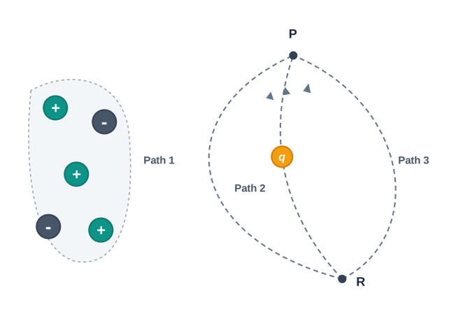
Fig. 2.2 – Path-independence of work done by an electrostatic field.
Defining the potential
Starting from the work relation of Eq. (2.1), the work done by the external force in bringing a unit positive charge from point R to point P is:
\[V\_P - V\_R = \\frac{U\_P - U\_R}{q} \\tag{2.4}\]
where \(V\_P\) and \(V\_R\) are the electrostatic potentials at P and R respectively, and \(U\_P - U\_R\) is the potential energy difference for a charge \(q\) moved between the same two points. As before, it is not the absolute value of the potential but the potential difference between two points that is physically significant.
As we did for potential energy, we choose the potential to be zero at infinity. With this choice, Eq. (2.4) tells us something clean and memorable: the work done by an external force in bringing a unit positive charge from infinity to a point is simply the electrostatic potential \(V\) at that point.
This answers what a statement like “this point is at 100 volts” really means. It says that to carry one unit of positive charge from infinity — the agreed zero level — up to that point, an external agent must do 100 joules of work per coulomb. The reference “from where” is always infinity, where the potential is taken as zero. The SI unit of potential is therefore the volt (V), defined as one joule per coulomb: \(1\\ \\text{V} = 1\\ \\text{J C}^{-1}\).
A note of caution
The same qualifying remarks we made for potential energy apply here to potential. To measure the work per unit test charge properly, we should really take an infinitesimal test charge \(\\delta q\), find the small work \(\\delta W\) done in bringing it from infinity to the point, and take the ratio \(\\delta W / \\delta q\). Using a vanishingly small test charge ensures it does not disturb the very field we are trying to measure. And at every point along the path, the external force must be kept equal and opposite to the electrostatic force on the test charge, so that the charge moves without acceleration.
2.3 Potential due to a Point Charge
Having defined what electrostatic potential means, we now put it to work in the simplest possible case: a single point charge. Our goal is to find a formula for the potential \(V\) at any point due to one isolated charge.
Consider a point charge \(Q\) placed at the origin, as shown in Fig. 2.3. To keep the discussion definite, take \(Q\) to be positive. We want the potential at some point P whose position vector from the origin is \(\\vec{r}\) — in other words, P lies at a distance \(r\) from the charge.
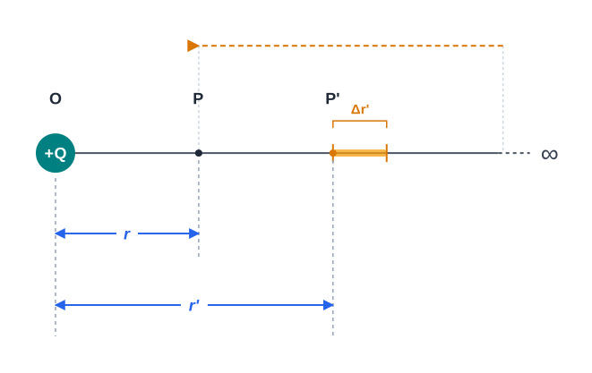
Fig. 2.3 – Calculating potential due to a point charge.
By definition, the potential at P is the work done in bringing a unit positive charge from infinity up to P. Since \(Q > 0\), the incoming test charge is pushed outward by repulsion, so an external agent must do positive work to move it inward. And because the work is independent of the path (a result we established in the last section), we are free to choose the most convenient path — a straight, radial line running from infinity directly in to P.
Building the work step by step
Consider an intermediate point P′ on this path, at a distance \(r'\) from the charge. The electrostatic force on a unit positive charge sitting there is given by Coulomb’s law:
\[\\frac{Q \\times 1}{4\\pi\\varepsilon\_0, r'^2},\\hat{\\mathbf{r}}' \\tag{2.5}\]
where \(\\hat{\\mathbf{r}}'\) is the unit vector pointing outward along OP′, \(\\varepsilon\_0\) is the permittivity of free space, and the combination \(\\dfrac{1}{4\\pi\\varepsilon\_0}\) has the value \(9\\times10^{9}\\ \\text{N m}^2,\\text{C}^{-2}\). The distance \(r'\) is in metres and the force is in newtons.
Now move the test charge inward by a small step, from \(r'\) to \(r' + \\Delta r'\). The small amount of work done against the repulsive force in this step is:
\[\\Delta W = -\\frac{Q}{4\\pi\\varepsilon\_0, r'^2},\\Delta r' \\tag{2.6}\]
The minus sign deserves a word of explanation. As the charge moves inward, its distance from \(Q\) shrinks, so \(\\Delta r'\) is negative. The work done against repulsion, however, must come out positive. The minus sign is precisely what makes \(\\Delta W\) positive when \(\\Delta r'\) is negative — so the sign is not a typo but a careful piece of bookkeeping.
To get the total work, we add up all these little steps from the starting point \(r' = \\infty\) down to the finishing point \(r' = r\). Adding up infinitely many small steps is exactly what integration does:
\[W = -\\int\_\\infty^r \\frac{Q}{4\\pi\\varepsilon\_0, r'^2},dr' = \\frac{Q}{4\\pi\\varepsilon\_0, r'}\\bigg|\_\\infty^r = \\frac{Q}{4\\pi\\varepsilon\_0, r} \\tag{2.7}\]
(The term at the infinity limit vanishes, since \(1/r' \\to 0\) as \(r' \\to \\infty\) — another payoff of choosing infinity as our zero.) By definition, this total work is the potential at P due to the charge \(Q\):
\[V(r) = \\frac{Q}{4\\pi\\varepsilon\_0, r} \\tag{2.8}\]
Here \(V\) is in volts when \(Q\) is in coulombs and \(r\) is in metres. This compact formula is one of the most important results in the whole chapter.
What the formula tells us
Although we derived Eq. (2.8) assuming \(Q > 0\), it holds for a charge of any sign. For a negative charge, \(Q < 0\), so the potential \(V\) comes out negative. Physically this makes sense: for \(Q < 0\), the force on an incoming positive test charge is attractive, so the external agent actually does negative work bringing it in — equivalently, the electric force itself does positive work, because now the force and the displacement point the same way. The formula automatically captures this through the sign of \(Q\).
Notice also that Eq. (2.8) is fully consistent with our choice that the potential is zero at infinity: as \(r \\to \\infty\), \(V \\to 0\).
Figure 2.4 shows how the potential and the field of a point charge fall off with distance. The potential varies as \(1/r\) (blue curve), while the electric field varies more steeply as \(1/r^2\) (black curve).
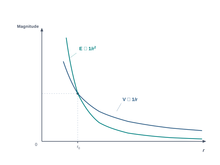
Fig. 2.4 – Variation of potential and electric field with distance.
2.4 Potential due to an Electric Dipole
We now move from a single charge to a slightly richer arrangement: the electric dipole. You met this object in the previous chapter, but let us recall what it is.
An electric dipole is a pair of equal and opposite charges, \(+q\) and \(-q\), separated by a small distance \(2a\). Its total charge is zero. Even so, the separation of the charges gives it an important vector property called the dipole moment, written \(\\vec{p}\). Its magnitude is \(q \\times 2a\), and it points along the line from the negative charge to the positive charge, as shown in Fig. 2.5.
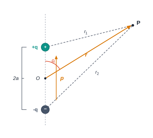
Fig. 2.5 – Geometry for calculating the potential of a dipole.
From the last chapter you also know that the field of a dipole depends not only on how far away the point is, but also on the angle between the position vector \(\\vec{r}\) and the dipole moment \(\\vec{p}\). And unlike a single charge, whose field falls off as \(1/r^2\), a dipole’s field falls off more steeply, as \(1/r^3\). Our task now is to find the dipole’s potential and to contrast it with that of a single charge.
Using superposition
Take the origin at the centre of the dipole. The electric field of the two charges obeys the superposition principle — the total field is the vector sum of the individual fields. Since potential is built from the work done by the field, potential also obeys superposition, but even more simply: potentials are ordinary numbers (scalars), so we just add them algebraically.
The potential at a point P is therefore the sum of the potentials due to \(+q\) and \(-q\):
\[V = \\frac{1}{4\\pi\\varepsilon\_0}\\left(\\frac{q}{r\_1} - \\frac{q}{r\_2}\\right) \\tag{2.9}\]
where \(r\_1\) and \(r\_2\) are the distances of P from \(+q\) and \(-q\) respectively.
Simplifying for a distant point
From the geometry of Fig. 2.5, the law of cosines gives:
\[r\_1^2 = r^2 + a^2 - 2ar\\cos\\theta\] \[r\_2^2 = r^2 + a^2 + 2ar\\cos\\theta \\tag{2.10}\]
These expressions are exact but clumsy. In almost every practical case the point P is far from the dipole, so we take \(r \\gg a\) and keep only terms up to the first order in the small ratio \(a/r\). Dropping the tiny \(a^2/r^2\) term:
\[r\_1^2 = r^2\\left(1 - \\frac{2a\\cos\\theta}{r} + \\frac{a^2}{r^2}\\right) \\cong r^2\\left(1 - \\frac{2a\\cos\\theta}{r}\\right) \\tag{2.11}\]
\[r\_2^2 \\cong r^2\\left(1 + \\frac{2a\\cos\\theta}{r}\\right) \\tag{2.12}\]
Now we need \(1/r\_1\) and \(1/r\_2\), not \(r\_1^2\) and \(r\_2^2\). Here we use the binomial approximation: for any small quantity \(x\), \((1+x)^n \\approx 1 + nx\). Taking \(n = -1/2\) (because \(1/r\_1 = (r\_1^2)^{-1/2}\)), and keeping only first order in \(a/r\):
\[\\frac{1}{r\_1} \\cong \\frac{1}{r}\\left(1 - \\frac{2a\\cos\\theta}{r}\\right)^{-1/2} \\cong \\frac{1}{r}\\left(1 + \\frac{a}{r}\\cos\\theta\\right) \\tag{2.13a}\]
\[\\frac{1}{r\_2} \\cong \\frac{1}{r}\\left(1 + \\frac{2a\\cos\\theta}{r}\\right)^{-1/2} \\cong \\frac{1}{r}\\left(1 - \\frac{a}{r}\\cos\\theta\\right) \\tag{2.13b}\]
Substituting these into Eq. (2.9) and using \(p = 2qa\), the two constant terms cancel and the two \(\\cos\\theta\) terms add, leaving:
\[V = \\frac{q}{4\\pi\\varepsilon\_0}\\frac{2a\\cos\\theta}{r^2} = \\frac{p\\cos\\theta}{4\\pi\\varepsilon\_0, r^2} \\tag{2.14}\]
Finally, since \(\\vec{p}\) makes angle \(\\theta\) with \(\\vec{r}\), the product \(p\\cos\\theta\) is exactly the dot product \(\\vec{p}\\cdot\\hat{\\mathbf{r}}\), where \(\\hat{\\mathbf{r}}\) is the unit vector along OP. So the potential of a dipole can be written compactly as:
\[V = \\frac{1}{4\\pi\\varepsilon\_0}\\frac{\\vec{p}\\cdot\\hat{\\mathbf{r}}}{r^2}; \\qquad (r \\gg a) \\tag{2.15}\]
Equation (2.15) is only approximately true for real dipoles, and only when the point is far compared with the dipole’s size, so that the higher-order terms in \(a/r\) can be neglected. For an idealised point dipole — one whose size shrinks to zero while \(p\) is kept fixed — Eq. (2.15) becomes exact at all distances.
Reading off special cases
From Eq. (2.15), the potential on the dipole axis (where \(\\theta = 0\) or \(\\theta = \\pi\), so \(\\cos\\theta = \\pm 1\)) is:
\[V = \\pm\\frac{1}{4\\pi\\varepsilon\_0}\\frac{p}{r^2} \\tag{2.16}\]
with the positive sign for \(\\theta = 0\) (the end nearer the \(+q\) charge) and the negative sign for \(\\theta = \\pi\). In the equatorial plane (\(\\theta = \\pi/2\)), \(\\cos\\theta = 0\), so the potential is exactly zero.
Contrasting a dipole with a single charge
Comparing the dipole result, Eq. (2.15), with the single-charge result, Eq. (2.8), brings out two important differences.
First, the potential of a dipole depends not just on the distance \(r\) but also on the angle between the position vector \(\\vec{r}\) and the dipole moment \(\\vec{p}\). It is, however, axially symmetric about \(\\vec{p}\): if you rotate the position vector \(\\vec{r}\) around the axis of \(\\vec{p}\) while keeping \(\\theta\) fixed, all the points you sweep out lie on a cone and share the same potential.
Second, the dipole potential falls off with distance as \(1/r^2\), whereas a single charge’s potential falls off only as \(1/r\). The dipole’s potential dies away faster because, from far away, the \(+q\) and \(-q\) charges nearly cancel — their leading \(1/r\) contributions wipe each other out, leaving the weaker \(1/r^2\) term. You can look back at Fig. 2.4, where the shapes of the \(1/r\) and \(1/r^2\) curves were drawn in another context, to picture how much more rapidly the \(1/r^2\) curve drops.
2.5 Potential due to a System of Charges
So far we have found the potential of one point charge and of a dipole. Real situations usually involve many charges at once. Happily, the rule for combining them is the simplest we could hope for.
Consider a system of charges \(q\_1, q\_2, \\ldots, q\_n\) located at positions with vectors \(\\vec{r}\_1, \\vec{r}\_2, \\ldots, \\vec{r}\_n\) from some chosen origin, as shown in Fig. 2.6. We want the potential at a point P.

Fig. 2.6 – Potential at a point due to a system of charges.
The potential \(V\_1\) at P due to the charge \(q\_1\) alone is given by our point-charge formula:
\[V\_1 = \\frac{1}{4\\pi\\varepsilon\_0}\\frac{q\_1}{r\_{1P}}\]
where \(r\_{1P}\) is the distance between \(q\_1\) and P. Likewise, the potentials due to \(q\_2\) and \(q\_3\) are:
\[V\_2 = \\frac{1}{4\\pi\\varepsilon\_0}\\frac{q\_2}{r\_{2P}}, \\qquad V\_3 = \\frac{1}{4\\pi\\varepsilon\_0}\\frac{q\_3}{r\_{3P}}\]
with \(r\_{2P}\) and \(r\_{3P}\) the distances of P from \(q\_2\) and \(q\_3\), and so on for the rest.
The superposition principle for potential
Because potential is a scalar, the total potential at P is just the ordinary algebraic sum of the separate potentials — no vector diagrams, no angles, no components:
\[V = V\_1 + V\_2 + \\cdots + V\_n \\tag{2.17}\]
\[V = \\frac{1}{4\\pi\\varepsilon\_0}\\left(\\frac{q\_1}{r\_{1P}} + \\frac{q\_2}{r\_{2P}} + \\cdots + \\frac{q\_n}{r\_{nP}}\\right) \\tag{2.18}\]
Continuous charge distributions
Sometimes charge is spread smoothly over a region rather than sitting at a few points. Such a distribution is described by a charge density \(\\rho(\\vec{r})\) — the charge per unit volume at each location. To handle it, we simply extend the summation idea. We chop the region into tiny volume elements, each of size \(\\Delta v\) and carrying a small charge \(\\rho,\\Delta v\). We find the potential due to each little element as if it were a point charge, and then sum — or, strictly speaking, integrate — over all of them to get the total potential of the whole distribution.
Potential of a uniformly charged spherical shell
A particularly useful case, which you met in the previous chapter, is a uniformly charged spherical shell of total charge \(q\) and radius \(R\). There we found that the field outside the shell behaves exactly as if the entire charge were squeezed into a point at the centre. The potential outside the shell is therefore the same as that of a point charge:
\[V = \\frac{1}{4\\pi\\varepsilon\_0}\\frac{q}{r} \\qquad (r \\geq R) \\tag{2.19a}\]
Inside the shell, the field is zero everywhere. Since the field is what does work on a moving charge, no work is needed to move a charge around inside the shell — which means the potential cannot change from point to point inside. The potential is therefore constant throughout the interior, and by continuity it must equal its value right at the surface (put \(r = R\)):
\[V = \\frac{1}{4\\pi\\varepsilon\_0}\\frac{q}{R} \\tag{2.19b}\]
(The reasoning that a zero field forces a constant potential is developed carefully in Section 2.6.)
Two charges \(3\\times10^{-8}\\ \\text{C}\) and \(-2\\times10^{-8}\\ \\text{C}\) are located \(15\\ \\text{cm}\) apart. At what point on the line joining the two charges is the electric potential zero? Take the potential at infinity to be zero.
Solution
Let us place the origin O at the positive charge and take the line joining the charges as the \(x\)-axis, with the negative charge on the right (see Fig. 2.7). Let P be the required point at coordinate \(x\), which must be positive (there is no way for the two potentials to cancel for \(x < 0\), since there the nearer charge is the larger positive one).
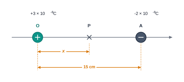
[Caption:] Fig. 2.7 – Finding the zero-potential point between two charges. [/Caption:]
If P lies between O and A, the total potential being zero gives:
\[\\frac{1}{4\\pi\\varepsilon\_0}\\left\[\\frac{3\\times10^{-8}}{x\\times10^{-2}} - \\frac{2\\times10^{-8}}{(15-x)\\times10^{-2}}\\right] = 0\]
where \(x\) is measured in cm. This simplifies to:
\[\\frac{3}{x} - \\frac{2}{15-x} = 0\]
which gives \(x = 9\\ \\text{cm}\).
If instead P lies on the extension of the line beyond A, the condition becomes:
\[\\frac{3}{x} - \\frac{2}{x-15} = 0\]
which gives \(x = 45\\ \\text{cm}\).
Thus the electric potential is zero at two points: \(9\\ \\text{cm}\) and \(45\\ \\text{cm}\) from the positive charge, both on the side towards the negative charge. Note that this whole calculation relied on our convention that the potential is zero at infinity.
Figures 2.8(a) and (b) show the field lines of a positive and a negative point charge respectively. In (a), point P is nearer the positive charge than point Q; in (b), point A is nearer the negative charge than point B.
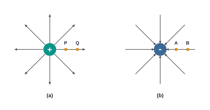
[Caption:] Fig. 2.8 – Points in the field of (a) a positive and (b) a negative charge. [/Caption:]
(a) Give the signs of the potential differences \(V\_P - V\_Q\) and \(V\_B - V\_A\).
(b) Give the sign of the potential energy difference of a small negative charge between the points Q and P, and between A and B.
(c) Give the sign of the work done by the field in moving a small positive charge from Q to P.
(d) Give the sign of the work done by an external agency in moving a small negative charge from B to A.
(e) Does the kinetic energy of a small negative charge increase or decrease in going from B to A?
Solution
Since \(V \\propto \\dfrac{1}{r}\) for a point charge, and P is nearer the positive charge, \(V\_P > V\_Q\); hence \((V\_P - V\_Q)\) is positive. In (b), \(V\_B\) is less negative than \(V\_A\) (B is farther from the negative charge), so \(V\_B > V\_A\) and \((V\_B - V\_A)\) is positive.
A small negative charge is attracted towards a positive charge, so it moves from higher to lower potential energy. Therefore the potential energy difference of a small negative charge between Q and P is positive. Similarly, \((\\text{P.E.})\_A > (\\text{P.E.})\_B\), so that potential energy difference is positive as well.
To move a small positive charge from Q to P, an external agency must do work against the electric field. Therefore the work done by the field is negative.
To move a small negative charge from B to A, work has to be done by the external agency. It is positive.
Because of the force of repulsion on the negative charge, its velocity decreases, and hence its kinetic energy decreases in going from B to A.
2.6 Equipotential Surfaces
We have been calculating the potential \(V\) at individual points. A powerful way to picture the potential over a whole region is to join up all the points that share the same value of \(V\). The surface formed this way is called an equipotential surface.
Equipotentials of a single charge
For a single point charge \(q\), the potential is \(V = \\dfrac{1}{4\\pi\\varepsilon\_0}\\dfrac{q}{r}\). This depends only on the distance \(r\) from the charge, so \(V\) is constant wherever \(r\) is constant. The set of all points at a fixed distance from the charge is a sphere. Hence the equipotential surfaces of a point charge are a family of concentric spheres centred on the charge, as shown in Fig. 2.9(a).
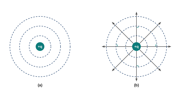
Fig. 2.9 – (a) Equipotential surfaces and (b) field lines for a point charge.
Recall from the previous chapter that the field lines of a single charge are straight radial lines, pointing outward from a positive charge or inward to a negative one, as in Fig. 2.9(b). Compare the two pictures: the radial field lines cut through the spherical equipotentials at right angles at every point. This is no coincidence.
Field is always perpendicular to equipotential surfaces
The relationship we just noticed for a single charge holds for any arrangement of charges.
The proof is short and worth following. Suppose, for contradiction, that the field were not perpendicular to the equipotential surface at some point. Then the field would have a non-zero component lying along the surface. Moving a test charge along the surface, against that tangential component, would require some work to be done.
But this contradicts the very meaning of an equipotential surface: since every point on it has the same potential, the potential difference between any two points on it is zero, and so no work is needed to move a charge from one point of the surface to another. The only way to avoid the contradiction is for the field to have no component along the surface at all — that is, the field must be entirely perpendicular to the equipotential surface at every point.
Equipotential surfaces give us a second, complementary way to visualise a charge configuration — alongside the familiar picture of electric field lines. Wherever you can draw one picture, you can draw the other, since the two families always cross at right angles.
Some common cases
For a uniform electric field \(\\vec{E}\) directed along the \(x\)-axis, the equipotential surfaces are flat planes perpendicular to the \(x\)-axis — that is, planes parallel to the \(y\)–\(z\) plane, as in Fig. 2.10. Since the field has the same strength and direction everywhere, these equally spaced planes are all parallel to one another.
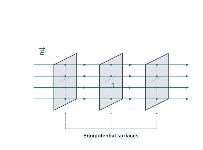
Fig. 2.10 – Equipotential surfaces for a uniform electric field.
The equipotential surfaces become more interesting for arrangements with more than one charge. Figure 2.11 shows the equipotentials for (a) a dipole and (b) two identical positive charges. Near each individual charge the surfaces are almost spherical, but farther out they distort into more complex shapes that reflect the combined potential.
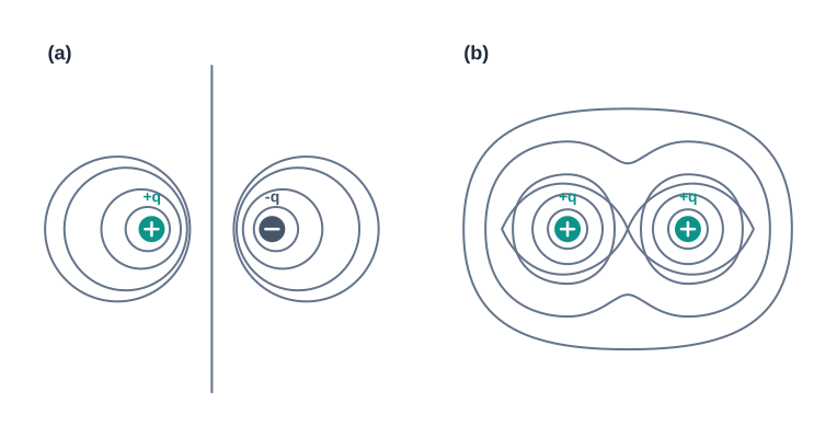
Fig. 2.11 – Equipotential surfaces for (a) a dipole and (b) two identical positive charges.
2.6.1 Relation between Field and Potential
Field and potential are two descriptions of the same electrostatic situation, so they must be linked. In this section we make that link precise: we show exactly how to get the field from the way the potential changes in space.
Consider two equipotential surfaces A and B lying very close together, as shown in Fig. 2.12. Let surface A be at potential \(V\) and surface B at potential \(V + \\delta V\), where \(\\delta V\) is the small change in potential as we move in the direction of the electric field \(\\vec{E}\). Let P be a point on surface B, and let \(\\delta l\) be the perpendicular distance from P across to surface A.
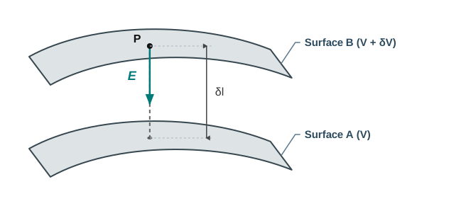
Fig. 2.12 – Relation between electric field and potential gradient.
Now imagine moving a unit positive charge along this perpendicular, from surface B across to surface A, against the electric field. Since the displacement \(\\delta l\) is taken along the field direction, the work done in this move is simply:
\[\\text{work} = |\\vec{E}|,\\delta l\]
But this work must also equal the potential difference the charge is carried through, \(V\_A - V\_B\). Since \(V\_A = V\) and \(V\_B = V + \\delta V\):
\[|\\vec{E}|,\\delta l = V - (V + \\delta V) = -\\delta V\]
which rearranges to:
\[|\\vec{E}| = -\\frac{\\delta V}{\\delta l} \\tag{2.20}\]
Here \(\\delta V\) is measured in volts and \(\\delta l\) in metres, so the field comes out in volts per metre (V m⁻¹) — a unit fully equivalent to the newton per coulomb (N C⁻¹) you used in the last chapter.
Because the potential decreases as we move along the field, \(\\delta V\) is negative, so we can write \(\\delta V = -|\\delta V|\). Substituting this into Eq. (2.20) turns the two minus signs into a plus:
\[|\\vec{E}| = -\\frac{\\delta V}{\\delta l} = +\\frac{|\\delta V|}{\\delta l} \\tag{2.21}\]
The quantity \(\\dfrac{|\\delta V|}{\\delta l}\) — the rate at which the potential changes with distance — is called the potential gradient.
What this tells us
Equation (2.21) gives us two important conclusions about how field and potential are related.
This relation is extremely useful in practice: if you know how the potential varies through a region, you can immediately deduce both the direction and the strength of the field, without having to add up contributions from every charge. The field is strongest exactly where the equipotential surfaces are packed most tightly together, because that is where the potential changes fastest over a short distance.
2.7 Potential Energy of a System of Charges
Earlier we found the potential energy of a single charge sitting in a field made by others. We now ask a broader question: how much energy is locked up in an entire arrangement of charges, taken as a whole? This is the work an external agency must do to assemble the charges, starting with them infinitely far apart.
Two charges
Consider the simplest case: two charges \(q\_1\) and \(q\_2\), which we want to place at positions \(\\vec{r}\_1\) and \(\\vec{r}\_2\), as in Fig. 2.13. Imagine them both beginning at infinity, and bring them in one at a time.
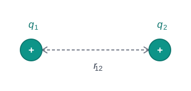
Fig. 2.13 – Two point charges separated by distance r₁₂.
Bring \(q\_1\) in first. Space is completely empty, so there is no field to push against — the work needed to bring \(q\_1\) from infinity to \(\\vec{r}\_1\) is zero. Once in place, \(q\_1\) sets up a potential in the surrounding space:
\[V\_1 = \\frac{1}{4\\pi\\varepsilon\_0}\\frac{q\_1}{r\_{1P}}\]
where \(r\_{1P}\) is the distance of a point P from \(q\_1\).
Now bring \(q\_2\) in. By the definition of potential, the work done in carrying \(q\_2\) from infinity to \(\\vec{r}\_2\) equals \(q\_2\) times the potential there due to \(q\_1\):
\[\\text{work done on } q\_2 = \\frac{1}{4\\pi\\varepsilon\_0}\\frac{q\_1 q\_2}{r\_{12}}\]
where \(r\_{12}\) is the distance between the two charges. Since the electrostatic force is conservative, this work is stored as the potential energy of the system:
\[U = \\frac{1}{4\\pi\\varepsilon\_0}\\frac{q\_1 q\_2}{r\_{12}} \\tag{2.22}\]
Here \(U\) is in joules when the charges are in coulombs and \(r\_{12}\) in metres.
Notice we could equally have brought \(q\_2\) in first and \(q\_1\) later — the answer \(U\) would be identical. In fact, because the work is path-independent, the potential energy is completely unaffected by the order or the route used to assemble the charges. It depends only on the final arrangement.
The meaning of the sign
Equation (2.22) works for charges of any sign, and the sign of \(U\) carries real physical meaning.
If \(q\_1 q\_2 > 0\) (like charges), the potential energy is positive. This makes sense: like charges repel, so positive work must be done against the repulsion to push them from infinity to a finite separation, and that positive work is stored.
If \(q\_1 q\_2 < 0\) (unlike charges), the force is attractive. To pull them apart — from their given positions back out to infinity — an external agency would have to do positive work against the attraction. Equivalently, assembling them (the reverse process) involves negative work, so the stored potential energy is negative.
Three charges
The same step-by-step method extends to any number of charges. Take three charges \(q\_1\), \(q\_2\), \(q\_3\) at \(\\vec{r}\_1\), \(\\vec{r}\_2\), \(\\vec{r}\_3\), as in Fig. 2.14.
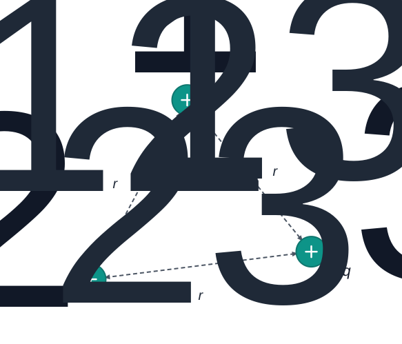
Fig. 2.14 – Potential energy of a three-charge system.
Bringing \(q\_1\) in requires no work. Bringing \(q\_2\) in against the field of \(q\_1\) requires:
\[q\_2 V\_1(\\vec{r}*2) = \\frac{1}{4\\pi\\varepsilon\_0}\\frac{q\_1 q\_2}{r*{12}} \\tag{2.23}\]
Now \(q\_1\) and \(q\_2\) together produce a potential which, at any point P, is:
\[V\_{1,2} = \\frac{1}{4\\pi\\varepsilon\_0}\\left(\\frac{q\_1}{r\_{1P}} + \\frac{q\_2}{r\_{2P}}\\right) \\tag{2.24}\]
Bringing \(q\_3\) in from infinity therefore requires \(q\_3\) times this potential evaluated at \(\\vec{r}\_3\):
\[q\_3 V\_{1,2}(\\vec{r}*3) = \\frac{1}{4\\pi\\varepsilon\_0}\\left(\\frac{q\_1 q\_3}{r*{13}} + \\frac{q\_2 q\_3}{r\_{23}}\\right) \\tag{2.25}\]
Adding the work of every step gives the total potential energy of the three-charge system:
\[U = \\frac{1}{4\\pi\\varepsilon\_0}\\left(\\frac{q\_1 q\_2}{r\_{12}} + \\frac{q\_1 q\_3}{r\_{13}} + \\frac{q\_2 q\_3}{r\_{23}}\\right) \\tag{2.26}\]
Note the pattern: there is exactly one term for each pair of charges. Once again, because the electrostatic force is conservative, this final expression is independent of the order in which the charges are assembled. The potential energy is a property of the present arrangement — the state the charges are in — and not of the history of how they got there.
Four charges are arranged at the corners of a square ABCD of side \(d\), as shown in Fig. 2.15: \(+q\) at A, \(-q\) at B, \(+q\) at C, and \(-q\) at D. (a) Find the work required to put this arrangement together. (b) A charge \(q\_0\) is then brought to the centre E of the square, with the four corner charges held fixed. How much extra work is needed to do this?
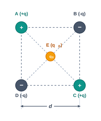
[Caption:] Fig. 2.15 – Four charges arranged at the corners of a square. [/Caption:]
Solution
Since the work depends only on the final arrangement and not on how it is built, we compute it for one convenient order: bring \(+q\) to A first, then \(-q\), \(+q\), and \(-q\) to B, C, and D in turn. The total work is found in steps.
Work to bring \(+q\) to A when no other charge is present: this is zero.
- Work to bring \(-q\) to B when \(+q\) is at A. This equals (charge at B) × (potential at B due to the charge at A), where A and B are a side length \(d\) apart:
\[= -q\\left(\\frac{q}{4\\pi\\varepsilon\_0 d}\\right) = -\\frac{q^2}{4\\pi\\varepsilon\_0 d}\]
- Work to bring \(+q\) to C when \(+q\) is at A and \(-q\) is at B. The diagonal A–C has length \(d\\sqrt{2}\) and the side B–C has length \(d\):
\[= +q\\left(\\frac{+q}{4\\pi\\varepsilon\_0 d\\sqrt{2}} + \\frac{-q}{4\\pi\\varepsilon\_0 d}\\right) = \\frac{-q^2}{4\\pi\\varepsilon\_0 d}\\left(1 - \\frac{1}{\\sqrt{2}}\\right)\]
- Work to bring \(-q\) to D when \(+q\) is at A, \(-q\) at B, and \(+q\) at C. Here A–D and C–D are sides of length \(d\), while B–D is the diagonal of length \(d\\sqrt{2}\):
\[= -q\\left(\\frac{+q}{4\\pi\\varepsilon\_0 d} + \\frac{-q}{4\\pi\\varepsilon\_0 d\\sqrt{2}} + \\frac{q}{4\\pi\\varepsilon\_0 d}\\right) = \\frac{-q^2}{4\\pi\\varepsilon\_0 d}\\left(2 - \\frac{1}{\\sqrt{2}}\\right)\]
Adding steps (i)–(iv), the total work required is:
\[= \\frac{-q^2}{4\\pi\\varepsilon\_0 d}\\left{(0) + (1) + \\left(1 - \\frac{1}{\\sqrt{2}}\\right) + \\left(2 - \\frac{1}{\\sqrt{2}}\\right)\\right}\]
\[= \\frac{-q^2}{4\\pi\\varepsilon\_0 d}\\left(4 - \\sqrt{2}\\right)\]
By definition, this is the total electrostatic potential energy of the four charges.
- The extra work needed to bring a charge \(q\_0\) to the centre E equals \(q\_0 \\times\) (the potential at E due to the four corner charges). Each corner is the same distance from E, and the charges are \(+q, -q, +q, -q\). The potential contributions of A and C (\(+q\) each) are exactly cancelled by those of B and D (\(-q\) each). So the potential at E is zero, and hence no work is required to bring any charge to the centre E.
2.8 Potential Energy in an External Field
2.8.1 Potential Energy of a Single Charge
In Section 2.7 we specified the source of the field completely — we knew every charge and where it sat — and we worked out the potential energy of that whole collection of charges. In this section we ask a related but genuinely different question: what is the potential energy of one charge \(q\) placed in a field that is already there?
This is, in fact, the very question that first led us to the idea of potential back in Sections 2.1 and 2.2. We return to it now mainly to make clear how it differs from the situation in Section 2.7.
The key difference: an external field
The crucial new feature is the word external. The field \(\\vec{E}\) here is not produced by the charge \(q\) whose energy we want. It is set up by other charges — the external sources — sitting somewhere else.
Often we do not even know the details of those sources. What we are handed instead is the external field \(\\vec{E}\), or equivalently the external potential \(V\), that they produce in the region of interest. We then assume that our charge \(q\) is too feeble to disturb these sources. This assumption holds if \(q\) is very small, or if the external sources are firmly held in place by other agencies. Even a sizeable \(q\) can be treated this way when the sources are very strong and far off (effectively at infinity), yet still produce a definite field in our region.
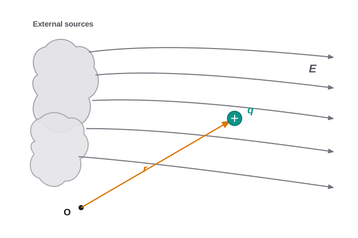
Fig. 2.16 – A single charge in an external electric field.
The formula
The external potential \(V\) may take different values at different points. By our standard definition, the potential \(V\) at a point P is the work done in bringing a unit positive charge from infinity to P (still taking the potential at infinity to be zero). So the work done in bringing a charge \(q\) from infinity to P in this external field is simply \(q\) times that:
\[\\text{work done} = qV\]
This work is stored as the potential energy of the charge \(q\). If the point P has position vector \(\\vec{r}\), we write:
\[\\text{Potential energy of } q \\text{ at } \\vec{r} = qV(\\vec{r}) \\tag{2.27}\]
where \(V(\\vec{r})\) is the external potential at the point \(\\vec{r}\).
The electron volt
Equation (2.27) leads naturally to a unit of energy that is used everywhere in atomic, nuclear, and particle physics. Suppose an electron, of charge \(q = e = 1.6\\times10^{-19}\\ \\text{C}\), is accelerated through a potential difference of \(\\Delta V = 1\) volt. From Eq. (2.27), it gains energy:
\[q,\\Delta V = 1.6\\times10^{-19}\\ \\text{J}\]
This amount of energy is defined as one electron volt, written \(1\\ \\text{eV}\).
Because atomic-scale energies are tiny in joules, physicists prefer the eV and its multiples:
\[1\\ \\text{keV} = 10^{3}\\ \\text{eV} = 1.6\\times10^{-16}\\ \\text{J}\] \[1\\ \\text{MeV} = 10^{6}\\ \\text{eV} = 1.6\\times10^{-13}\\ \\text{J}\] \[1\\ \\text{GeV} = 10^{9}\\ \\text{eV} = 1.6\\times10^{-10}\\ \\text{J}\] \[1\\ \\text{TeV} = 10^{12}\\ \\text{eV} = 1.6\\times10^{-7}\\ \\text{J}\]
(You first met this unit in Class XI Physics.)
2.8.2 Potential Energy of a System of Two Charges in an External Field
We now combine the two ideas we have just built: the mutual energy of charges (Section 2.7) and the energy of a charge in an external field (Section 2.8.1). The question is: what is the potential energy of a pair of charges \(q\_1\) and \(q\_2\), sitting at \(\\vec{r}\_1\) and \(\\vec{r}\_2\), when they are placed in an external field?
As before, we assemble the system one charge at a time and add up the work.
Bringing in \(q\_1\). Space already contains the external field, but no other charge of ours. So the only work is against the external field, which by Eq. (2.27) is \(q\_1 V(\\vec{r}\_1)\), where \(V\) is the external potential.
Bringing in \(q\_2\). This step is where the new subtlety appears. As \(q\_2\) is carried to \(\\vec{r}\_2\), it must be pushed against two fields at once: the external field, and the field now produced by the charge \(q\_1\) already in place.
The work against the external field is:
\[q\_2 V(\\vec{r}\_2)\]
and the work against the field due to \(q\_1\) is the familiar mutual term from Eq. (2.22):
\[\\frac{q\_1 q\_2}{4\\pi\\varepsilon\_0, r\_{12}}\]
where \(r\_{12}\) is the distance between the two charges. Because fields obey the superposition principle, we simply add these two contributions to get the total work of bringing \(q\_2\) into position:
\[\\text{work done in bringing } q\_2 \\text{ to } \\vec{r}\_2 = q\_2 V(\\vec{r}*2) + \\frac{q\_1 q\_2}{4\\pi\\varepsilon\_0, r*{12}} \\tag{2.28}\]
Adding the work of both steps gives the total potential energy of the system — the total work done in assembling the whole configuration:
\[U = q\_1 V(\\vec{r}\_1) + q\_2 V(\\vec{r}*2) + \\frac{q\_1 q\_2}{4\\pi\\varepsilon\_0, r*{12}} \\tag{2.29}\]
Read the three terms physically: the first two are the energies of \(q\_1\) and \(q\_2\) each interacting with the external field, and the last is the mutual energy of the two charges with each other. This clean separation — external terms plus one mutual term — is worth remembering, because exam problems often ask you to identify or compute just one part of it.
2.8.3 Potential Energy of a Dipole in an External Field
A dipole placed in an external field is a case worth studying on its own, because it turns up constantly — in molecules, in dielectrics (which we meet shortly), and in many devices. Here we find how much potential energy a dipole stores as it turns in a uniform external field.
Consider a dipole made of charges \(q\_1 = +q\) and \(q\_2 = -q\), placed in a uniform external field \(\\vec{E}\), as shown in Fig. 2.17.
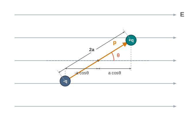
Fig. 2.17 – A dipole in a uniform external field.
Torque, not force
From the previous chapter, recall that in a uniform field the two forces on \(+q\) and \(-q\) are equal in size but opposite in direction, so the net force on the dipole is zero. However, these two forces act at different points, forming a couple that tends to rotate the dipole. The dipole therefore experiences a torque:
\[\\vec{\\tau} = \\vec{p}\\times\\vec{E} \\tag{2.30}\]
This torque tends to turn the dipole (unless \(\\vec{p}\) is already parallel or antiparallel to \(\\vec{E}\), when it vanishes).
Work done in rotating the dipole
To find the potential energy, imagine applying an external torque \(\\tau\_{ext}\) that exactly balances the field’s torque, so the dipole turns extremely slowly, without angular acceleration, from an angle \(\\theta\_0\) to an angle \(\\theta\_1\). The work done by this external torque is:
\[W = \\int\_{\\theta\_0}^{\\theta\_1}\\tau\_{ext}(\\theta),d\\theta = \\int\_{\\theta\_0}^{\\theta\_1} pE\\sin\\theta,d\\theta = pE\\left(\\cos\\theta\_0 - \\cos\\theta\_1\\right) \\tag{2.31}\]
This work is stored as the potential energy \(U(\\theta)\) of the dipole at inclination \(\\theta\). As always with potential energy, we are free to choose where \(U = 0\). The natural choice here is \(\\theta\_0 = \\pi/2\) — that is, we set the energy to zero when the dipole is perpendicular to the field. (The reason this choice is natural is explained just below.) With \(\\cos(\\pi/2) = 0\), Eq. (2.31) gives:
\[U(\\theta) = pE\\left(\\cos\\frac{\\pi}{2} - \\cos\\theta\\right) = -pE\\cos\\theta = -\\vec{p}\\cdot\\vec{E} \\tag{2.32}\]
The compact form \(U = -\\vec{p}\\cdot\\vec{E}\) tells a clear physical story. The energy is lowest (\(U = -pE\)) when \(\\theta = 0\), i.e. when the dipole is aligned with the field — this is the stable position the dipole naturally settles into. It is highest (\(U = +pE\)) when \(\\theta = \\pi\), pointing against the field — an unstable position. To turn the dipole away from alignment, an external agency must always do positive work.
An alternative derivation
The same result follows from Eq. (2.29), applied to the two charges \(+q\) and \(-q\) making up the dipole. That equation gives:
\[U'(\\theta) = q\[V(\\vec{r}\_1) - V(\\vec{r}\_2)] - \\frac{q^2}{4\\pi\\varepsilon\_0\\times 2a} \\tag{2.33}\]
where \(\\vec{r}\_1\) and \(\\vec{r}\_2\) are the positions of \(+q\) and \(-q\). Now, the potential difference \(V(\\vec{r}\_1) - V(\\vec{r}\_2)\) equals the work done in moving a unit positive charge against the field from \(\\vec{r}\_2\) to \(\\vec{r}\_1\). The displacement of \(+q\) relative to \(-q\), measured along the field, is \(2a\\cos\\theta\), so \(\[V(\\vec{r}\_1) - V(\\vec{r}\_2)] = -E\\times 2a\\cos\\theta\). Substituting:
\[U'(\\theta) = -pE\\cos\\theta - \\frac{q^2}{4\\pi\\varepsilon\_0\\times 2a} = -\\vec{p}\\cdot\\vec{E} - \\frac{q^2}{4\\pi\\varepsilon\_0\\times 2a} \\tag{2.34}\]
This \(U'(\\theta)\) differs from our earlier \(U(\\theta)\) only by the last term, which is a fixed constant for a given dipole (it is just the internal energy binding \(+q\) and \(-q\)). Since an additive constant does not affect potential energy, we may drop it, and Eq. (2.34) reduces exactly to Eq. (2.32).
We can now see why the choice \(\\theta\_0 = \\pi/2\) was natural. At \(\\theta = \\pi/2\) the dipole lies perpendicular to the field; then the work done against the external field in bringing \(+q\) and \(-q\) into place is equal and opposite for the two charges and cancels, i.e. \(q\[V(\\vec{r}\_1) - V(\\vec{r}\_2)] = 0\). So this orientation is the cleanest possible zero of potential energy.
2.9 Electrostatics of Conductors
You met conductors and insulators briefly in the previous chapter. We now study how conductors behave in electrostatic situations, and derive a set of results that are among the most useful in the whole subject.
What makes a conductor special
Conductors contain mobile charge carriers — charges free to move about. In a metal, these carriers are electrons. The outer (valence) electrons of the metal atoms break away and are free to roam within the metal, though they cannot leave it. These free electrons behave like a kind of “gas”: they collide with one another and with the ions, and move randomly in all directions. When an external field is applied, they drift, on average, against the direction of the field. Meanwhile the positive ions — the nuclei together with the tightly bound inner electrons — stay locked in their fixed lattice positions.
(In electrolytic conductors the carriers are both positive and negative ions, and their motion is influenced by chemical forces as well as by the electric field — a more involved case studied in the next chapter. Here we restrict ourselves to solid metallic conductors.)
With that picture in mind, here are the important results.
Result 1: Inside a conductor, the electrostatic field is zero
Take any conductor, charged or neutral, possibly sitting in an external field. In the static situation — when no current flows — the electric field is zero everywhere inside the conductor.
The reasoning is simple. A conductor is full of free electrons. If any field existed inside, those free charges would feel a force and start drifting — but that would be a current, contradicting the static assumption. So the free charges must have already rearranged themselves in exactly the way needed to make the internal field vanish. In fact, this can be taken as the defining property of a conductor.
Result 2: At the surface, the field is normal to the surface
Just at the surface of a charged conductor, the electrostatic field must be perpendicular (normal) to the surface at every point.
If the field had any component along the surface, the free charges sitting on the surface would feel a sideways push and would move — again a current, forbidden in the static case. So in equilibrium the field can have no tangential component; it must point straight out of (or into) the surface. (If a part of the surface carries no charge at all, the field there is zero even at the surface.)
Result 3: No excess charge inside — it all sits on the surface
A neutral conductor has equal amounts of positive and negative charge in every tiny region. When we give a conductor an excess charge, that excess can reside only on the surface.
This follows from Gauss’s law. Take any small closed surface \(S\) drawn entirely inside the conductor. Since the field is zero everywhere inside (Result 1), the electric flux through \(S\) is zero, and by Gauss’s law the net charge enclosed by \(S\) must be zero. But \(S\) can be shrunk down to surround any point we like, so there is no net charge at any interior point. Every bit of excess charge is therefore forced out onto the surface.
Result 4: The whole conductor is at one constant potential
The electrostatic potential is constant throughout the volume of a conductor, and takes that same value on its surface.
This follows directly from Results 1 and 2. Because the field is zero inside, and has no tangential component on the surface, no work is done in carrying a test charge anywhere within the conductor or across its surface. If no work is done, there is no potential difference — so every point inside and on the surface is at the same potential. (Just outside a charged conductor, however, the field is non-zero and normal to the surface, so the potential does change as you step off the surface.)
In a collection of several conductors, each one sits at its own constant potential, but that constant can differ from one conductor to another.
Result 5: The field just outside a charged conductor
At the surface of a charged conductor, the field is:
\[\\vec{E} = \\frac{\\sigma}{\\varepsilon\_0}\\hat{\\mathbf{n}} \\tag{2.35}\]
where \(\\sigma\) is the surface charge density (charge per unit area, in C m⁻²) and \(\\hat{\\mathbf{n}}\) is the outward unit normal to the surface.
To derive it, we use a small Gaussian pill box — a short cylinder of tiny cross-section \(\\delta S\) and negligible height — placed so it straddles the surface, partly inside and partly outside, as in Fig. 2.18. Just inside the surface the field is zero, and just outside it is normal to the surface with magnitude \(E\). So the only flux through the pill box comes from its outer flat face, equal to \(\\pm E,\\delta S\) (positive for \(\\sigma > 0\), negative for \(\\sigma < 0\)). The charge enclosed is \(\\sigma,\\delta S\).
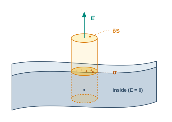
Fig. 2.18 – Gaussian pillbox at the surface of a charged conductor.
Applying Gauss’s law:
\[E,\\delta S = \\frac{|\\sigma|,\\delta S}{\\varepsilon\_0} \\quad\\Longrightarrow\\quad E = \\frac{|\\sigma|}{\\varepsilon\_0} \\tag{2.36}\]
Including the fact that the field is normal to the surface gives the vector form, Eq. (2.35). For \(\\sigma > 0\) the field points outward; for \(\\sigma < 0\) it points inward.
Result 6: Electrostatic shielding
Consider a conductor with a hollow cavity inside it, containing no charges. A remarkable result holds: the electric field inside that cavity is zero — no matter what shape the cavity has, no matter how much charge sits on the conductor, and no matter what external fields the conductor is placed in.
We have already proved a special case of this: the field inside a charged spherical shell is zero. That proof relied on the shell’s spherical symmetry, but the general result requires no such symmetry. Whether the conductor is charged, or has charges induced on it by an external field, all the charge ends up on the outer surface of the conductor, and the cavity stays completely field-free.
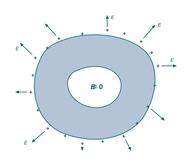
Fig. 2.19 – Electrostatic shielding in a hollow conductor.
This effect is called electrostatic shielding, and it has a valuable practical use: sensitive instruments can be protected from outside electrical disturbances by enclosing them in a conducting box. Figure 2.20 collects the key electrostatic properties of a conductor in one picture.
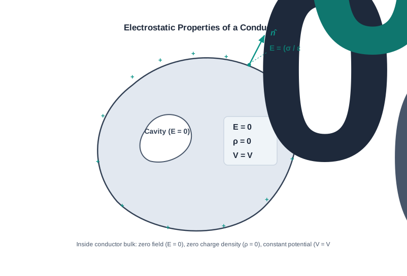
Fig. 2.20 – Key electrostatic properties of a conductor.
2.10 Dielectrics and Polarisation
Having seen how conductors behave in an electric field, we now turn to dielectrics — the insulating materials that behave very differently.
Conductors versus dielectrics: a contrast
Recall from Section 2.9 what happens when a conductor is placed in an external field. Its free charges move around and redistribute themselves until the field they create exactly cancels the external field inside the conductor. The net field inside a conductor becomes zero.
A dielectric cannot do this, because it has no free charges to move about. Instead, the external field acts on the bound charges within each molecule — stretching or re-orienting the molecules so that each acquires (or aligns) a dipole moment. The combined effect of all these molecular dipoles is to produce charges on the surface of the dielectric, whose field opposes the external field. But here is the key difference: this opposing field only reduces the external field inside the dielectric — it does not cancel it completely, as it would in a conductor, as suggested in Fig. 2.21.
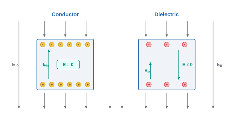
Fig. 2.21 – Internal fields in a conductor versus a dielectric.
How much the field is reduced depends on the nature of the dielectric, so we must look at what happens at the molecular level.
Polar and non-polar molecules
Molecules come in two kinds.
In a non-polar molecule, the centres of positive and negative charge coincide, so the molecule has no permanent dipole moment. Oxygen (\(\\text{O}\_2\)) and hydrogen (\(\\text{H}\_2\)) are examples — their symmetry keeps the charge centres together.
In a polar molecule, the centres of positive and negative charge are separated even when no external field is present, giving the molecule a permanent dipole moment. Ionic molecules such as HCl, and water (\(\\text{H}\_2\\text{O}\)), are common examples, as shown in Fig. 2.22.
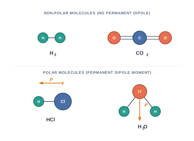
Fig. 2.22 – Non-polar and polar molecules.
How each type gets polarised
Non-polar molecules in a field. When an external field is applied, the positive and negative charges of a non-polar molecule are pushed in opposite directions. The displacement stops when the external force on the charges is balanced by the internal restoring force. The molecule thereby develops an induced dipole moment, and the dielectric is said to be polarised. In the simplest case — which we assume here — the induced dipole moment points along the field and is proportional to the field strength; substances obeying this are called linear isotropic dielectrics. The induced moments of all the molecules add up to give a net dipole moment of the whole dielectric.
Polar molecules in a field. A polar dielectric also acquires a net dipole moment in a field, but for a different reason. Without a field, its permanent dipoles point every which way because of random thermal motion, so their dipole moments cancel and the total is zero. When a field is applied, each dipole feels a torque nudging it toward the field direction. The result is a partial alignment, giving a net dipole moment along the field. The degree of alignment reflects a tug-of-war between two opposing influences: the dipole’s potential energy in the field, which favours alignment, and thermal energy, which disrupts it. (Polar molecules may also acquire a small induced moment as non-polar ones do, but for them the alignment effect usually dominates.) Figure 2.23 shows both mechanisms.
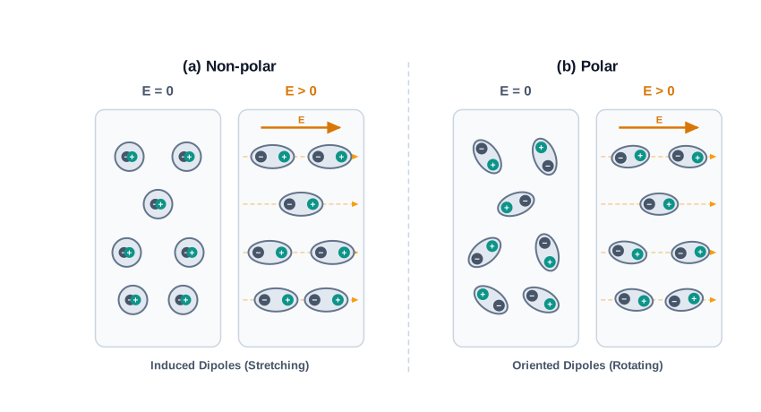
Fig. 2.23 – Polarisation of (a) non-polar and (b) polar dielectrics.
Polarisation and susceptibility
In every case — polar or non-polar — a dielectric develops a net dipole moment when placed in an external field. The dipole moment per unit volume of the dielectric is called its polarisation, denoted \(\\vec{P}\).
For linear isotropic dielectrics, the polarisation is proportional to the field:
\[\\vec{P} = \\varepsilon\_0 \\chi\_e, \\vec{E} \\tag{2.37}\]
Here \(\\chi\_e\) (Greek letter “chi”) is a constant characteristic of the material, called the electric susceptibility of the dielectric. It measures how readily the material polarises in response to a field. (It is possible to relate \(\\chi\_e\) to the molecular properties of the substance, but we shall not pursue that here.)
The induced surface charges
Now we can see how the polarised dielectric modifies the field inside it. Take a rectangular dielectric slab in a uniform external field \(\\vec{E}\_0\) parallel to two of its faces. The field produces a uniform polarisation \(\\vec{P}\), so every small volume element \(\\Delta v\) of the slab carries a dipole moment \(\\vec{P},\\Delta v\) pointing along the field. Each such element is macroscopically small yet contains a huge number of molecular dipoles.
Anywhere inside the slab, a volume element has no net charge, even though it has a net dipole moment. This is because the positive charge of one dipole sits right next to the negative charge of the neighbouring dipole, and they cancel. But at the surfaces of the slab that lie across the field, there is no neighbour to cancel with: as shown in Fig. 2.24, the positive ends of the dipoles are left unneutralised at one surface and the negative ends at the opposite surface. These unbalanced charges are the induced charges created by the external field.
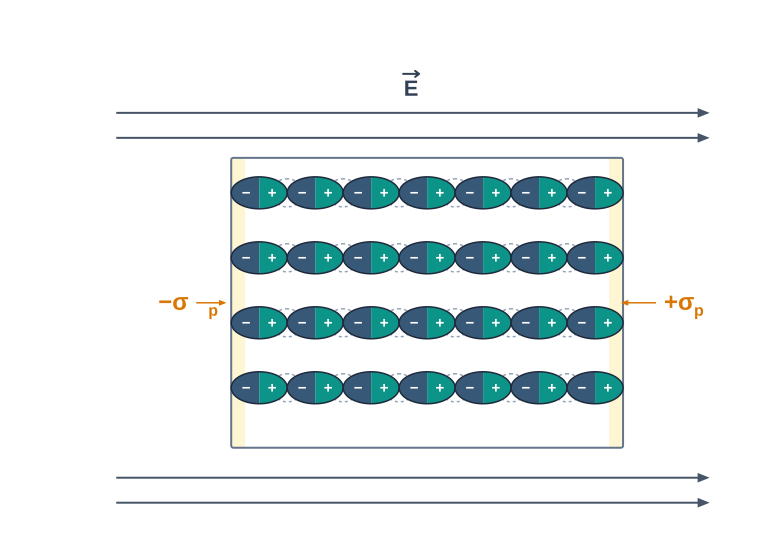
Fig. 2.24 – Induced surface charges on a polarised dielectric.
The polarised dielectric is therefore equivalent to two charged surfaces carrying induced surface charge densities \(+\\sigma\_p\) and \(-\\sigma\_p\). The field produced by these surface charges opposes the external field, so the total field inside the dielectric is reduced compared with the case when no dielectric is present. It is important to note that these surface charges \(\\pm\\sigma\_p\) come from bound charges — displaced or reoriented molecular charges — and not from free charges as in a conductor. This is why they cannot be tapped off as a current.
2.11 Capacitors and Capacitance
We now arrive at one of the most widely used devices in all of electronics: the capacitor. A capacitor is simply a system of two conductors separated by an insulator, as shown in Fig. 2.25.
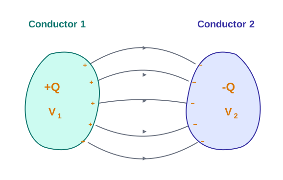
Fig. 2.25 – A general capacitor made of two conductors.
The two conductors carry charges \(Q\_1\) and \(Q\_2\) and sit at potentials \(V\_1\) and \(V\_2\). In practice, the arrangement we care about is the one where the two conductors carry equal and opposite charges, \(+Q\) and \(-Q\), with a potential difference \(V = V\_1 - V\_2\) between them. (Even a single conductor can act as a capacitor, its partner being taken at infinity.) The conductors are usually charged by connecting them to the two terminals of a battery.
The number \(Q\) is called the charge of the capacitor, although — as the name half-hides — it is really the charge on just one of the conductors; the total charge of the capacitor is zero, since the two charges are equal and opposite.
Defining capacitance
The electric field in the region between the conductors is proportional to the charge \(Q\). Double the charge, and the field everywhere doubles — this follows directly from the proportionality between field and charge built into Coulomb’s law and the superposition principle.
Now, the potential difference \(V\) is the work done per unit positive charge in carrying a test charge from conductor 2 to conductor 1 against this field. Since the field is proportional to \(Q\), the potential difference \(V\) is also proportional to \(Q\). Therefore the ratio \(Q/V\) is a constant:
\[C = \\frac{Q}{V} \\tag{2.38}\]
This constant \(C\) is called the capacitance of the capacitor.
The capacitance therefore depends only on the geometry of the two conductors — their shapes, sizes, and separation — and, as we shall see in Section 2.13, on the nature of the insulating material between them.
The unit: the farad
The SI unit of capacitance is the farad (F), defined as one coulomb per volt:
\[1\\ \\text{F} = 1\\ \\text{C V}^{-1}\]
A fixed capacitor is shown in circuit diagrams by two parallel lines, and a variable capacitor by the same symbol crossed by an arrow.
Why bigger capacitance is useful — and what limits it
From \(C = Q/V\), a large capacitance means a small voltage is enough to hold a large charge. This is of great practical value, because a high potential difference is dangerous: it means a strong electric field around the conductors.
If the field becomes strong enough, it can ionise the surrounding air, tearing electrons off air molecules. The charges so produced rush to the oppositely charged plates and partly neutralise them — in effect, the stored charge leaks away because the insulating medium has lost its insulating power.
The maximum field an insulating medium can withstand before it breaks down in this way is called its dielectric strength.
For air, the dielectric strength is about \(3\\times10^{6}\\ \\text{V m}^{-1}\). For a plate separation of about 1 cm, this corresponds to a potential difference of roughly \(3\\times10^{4}\\ \\text{V}\). So there is a definite ceiling on how much charge a given capacitor can hold: to store a lot of charge safely, its capacitance must be large enough that the required potential difference — and hence the field — stays below the breakdown limit.
In practice the farad is an enormous unit, so real capacitors are usually rated in its sub-multiples: the microfarad (\(1\\ \\mu\\text{F} = 10^{-6}\\ \\text{F}\)), the nanofarad (\(1\\ \\text{nF} = 10^{-9}\\ \\text{F}\)), and the picofarad (\(1\\ \\text{pF} = 10^{-12}\\ \\text{F}\)). Besides storing charge, the capacitor is a key element of most alternating-current circuits, as you will study in a later chapter.
2.12 The Parallel Plate Capacitor
The general definition \(C = Q/V\) tells us what capacitance is, but not how large it will be for a real device. To find an actual value, we need to choose a specific geometry and calculate. The simplest and most important case is the parallel plate capacitor.
A parallel plate capacitor consists of two large, flat, parallel conducting plates separated by a small distance, as in Fig. 2.26. For now we take the medium between the plates to be vacuum; the effect of filling it with a dielectric is the subject of the next section. Let \(A\) be the area of each plate and \(d\) the separation between them. The plates carry charges \(+Q\) and \(-Q\).
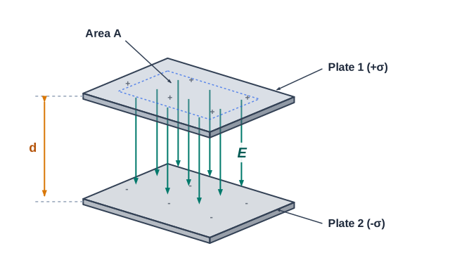
Fig. 2.26 – The parallel plate capacitor.
Field between the plates
Because the separation \(d\) is much smaller than the width of the plates (that is, \(d^2 \\ll A\)), each plate behaves, for points not too near the edges, like an infinite plane sheet of uniform charge. From the previous chapter, an infinite sheet of surface charge density \(\\sigma\) produces a field of magnitude \(\\sigma/2\\varepsilon\_0\) on each side. Plate 1 has \(\\sigma = Q/A\) and plate 2 has \(-\\sigma\). We add the fields of the two sheets in each region.
In the outer region I, above plate 1, the two fields point in opposite directions and cancel:
\[E = \\frac{\\sigma}{2\\varepsilon\_0} - \\frac{\\sigma}{2\\varepsilon\_0} = 0 \\tag{2.39}\]
In the outer region II, below plate 2, they again cancel:
\[E = \\frac{\\sigma}{2\\varepsilon\_0} - \\frac{\\sigma}{2\\varepsilon\_0} = 0 \\tag{2.40}\]
In the inner region between the plates, the two fields point the same way and add up:
\[E = \\frac{\\sigma}{2\\varepsilon\_0} + \\frac{\\sigma}{2\\varepsilon\_0} = \\frac{\\sigma}{\\varepsilon\_0} = \\frac{Q}{\\varepsilon\_0 A} \\tag{2.41}\]
The field points from the positive plate to the negative plate.
So the field is neatly localised between the plates and is uniform throughout that region. For real plates of finite size this is not quite true right at the edges, where the field lines bulge outward — an effect called fringing of the field. Fringing also means \(\\sigma\) is not perfectly uniform right at the edges. But provided \(d^2 \\ll A\), these edge effects can be ignored everywhere except very close to the boundary, and Eq. (2.41) holds well in the bulk.
Potential difference and capacitance
For a uniform field, the potential difference between the plates is simply the field multiplied by the distance between them:
\[V = E,d = \\frac{1}{\\varepsilon\_0}\\frac{Qd}{A} \\tag{2.42}\]
The capacitance follows from \(C = Q/V\):
\[C = \\frac{Q}{V} = \\frac{\\varepsilon\_0 A}{d} \\tag{2.43}\]
Just as expected, the capacitance depends only on the geometry — the plate area \(A\) and the separation \(d\) — and not on the charge or voltage. It grows with larger plate area and with smaller separation.
How big is a farad, really?
Let us plug in typical laboratory values, \(A = 1\\ \\text{m}^2\) and \(d = 1\\ \\text{mm}\):
\[C = \\frac{8.85\\times10^{-12}\\ \\text{C}^2,\\text{N}^{-1},\\text{m}^{-2} \\times 1\\ \\text{m}^2}{10^{-3}\\ \\text{m}} = 8.85\\times10^{-9}\\ \\text{F} \\tag{2.44}\]
(You can check the units work out, since \(1\\ \\text{F} = 1\\ \\text{C V}^{-1} = 1\\ \\text{C}^2,\\text{N}^{-1},\\text{m}^{-1}\).) Even these fairly large plates give only about 9 nanofarads — confirming that the farad is an enormous unit.
To drive the point home, let us ask how big the plates would have to be to reach a capacitance of \(1\\ \\text{F}\) with a separation of \(1\\ \\text{cm}\):
\[A = \\frac{Cd}{\\varepsilon\_0} = \\frac{1\\ \\text{F}\\times10^{-2}\\ \\text{m}}{8.85\\times10^{-12}\\ \\text{C}^2,\\text{N}^{-1},\\text{m}^{-2}} = 10^{9}\\ \\text{m}^2 \\tag{2.45}\]
That is a plate roughly 30 km on each side! Clearly, no ordinary flat-plate design can reach a whole farad.
2.13 Effect of Dielectric on Capacitance
In Section 2.10 we learned how a dielectric responds to a field, and in Section 2.12 we found the capacitance of a parallel plate capacitor with vacuum between the plates. Now we combine the two ideas: what happens to the capacitance when the gap is filled with a dielectric?
Take the same two large plates, each of area \(A\) and separated by \(d\), carrying charge \(\\pm Q\), i.e. surface charge density \(\\pm\\sigma\) (with \(\\sigma = Q/A\)). With vacuum between the plates, we already know the field and potential difference:
\[E\_0 = \\frac{\\sigma}{\\varepsilon\_0}, \\qquad V\_0 = E\_0 d\]
so the vacuum capacitance is:
\[C\_0 = \\frac{Q}{V\_0} = \\varepsilon\_0\\frac{A}{d} \\tag{2.46}\]
Inserting the dielectric
Now fill the gap completely with a dielectric. As we saw in Section 2.10, the field polarises the dielectric, and the effect is equivalent to two charged sheets at the surfaces of the dielectric carrying induced surface charge densities \(+\\sigma\_p\) and \(-\\sigma\_p\). These induced charges partly cancel the plate charges, so the net surface charge density responsible for the field inside is now \(\\pm(\\sigma - \\sigma\_p)\) rather than \(\\pm\\sigma\). The field in the dielectric is therefore:
\[E = \\frac{\\sigma - \\sigma\_p}{\\varepsilon\_0} \\tag{2.47}\]
which is smaller than the vacuum field \(E\_0\). The potential difference across the plates drops accordingly:
\[V = E,d = \\frac{\\sigma - \\sigma\_p}{\\varepsilon\_0}d \\tag{2.48}\]
For a linear dielectric, the induced density \(\\sigma\_p\) is proportional to the field \(E\_0\), and hence to \(\\sigma\). So the combination \((\\sigma - \\sigma\_p)\) is itself proportional to \(\\sigma\), and we can write:
\[\\sigma - \\sigma\_p = \\frac{\\sigma}{K} \\tag{2.49}\]
where \(K\) is a constant characteristic of the dielectric. Since \(\\sigma\_p\) is positive, \((\\sigma - \\sigma\_p)\) is less than \(\\sigma\), so \(K\) is greater than 1. Substituting into Eq. (2.48):
\[V = \\frac{\\sigma d}{\\varepsilon\_0 K} = \\frac{Qd}{A\\varepsilon\_0 K} \\tag{2.50}\]
The capacitance with the dielectric present is then:
\[C = \\frac{Q}{V} = \\frac{\\varepsilon\_0 K A}{d} \\tag{2.51}\]
Comparing with the vacuum result of Eq. (2.46), the capacitance has grown by exactly the factor \(K\).
Permittivity and dielectric constant
The product \(\\varepsilon\_0 K\) appears so often that it is given its own name, the permittivity of the medium, written \(\\varepsilon\):
\[\\varepsilon = \\varepsilon\_0 K \\tag{2.52}\]
For vacuum, \(K = 1\) and \(\\varepsilon = \\varepsilon\_0\), which is why \(\\varepsilon\_0\) is called the permittivity of vacuum (or free space). The dimensionless ratio:
\[K = \\frac{\\varepsilon}{\\varepsilon\_0} \\tag{2.53}\]
is called the dielectric constant of the substance, and as we just saw it is always greater than 1. Finally, dividing Eq. (2.51) by Eq. (2.46) gives a strikingly simple relation:
\[K = \\frac{C}{C\_0} \\tag{2.54}\]
Although we derived Eq. (2.54) for a parallel plate capacitor, the result is completely general — it holds for a capacitor of any shape, and can in fact be taken as the very definition of the dielectric constant of a substance.
2.14 Combination of Capacitors
Circuits rarely use a single capacitor in isolation. More often, several capacitors \(C\_1, C\_2, \\ldots, C\_n\) are connected together to give a system with some effective capacitance \(C\) — a single value that could replace the whole combination without changing how the circuit behaves. The effective capacitance depends on how the capacitors are wired together. We study the two simplest and most important arrangements: series and parallel.
2.14.1 Capacitors in Series
Figure 2.27 shows two capacitors \(C\_1\) and \(C\_2\) connected in series — that is, joined end to end so that the same charging path runs through both.
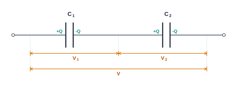
Fig. 2.27 – Two capacitors in series.
The outer left plate of \(C\_1\) and the outer right plate of \(C\_2\) are connected to the two terminals of a battery, receiving charges \(+Q\) and \(-Q\). It then follows that the inner plate of \(C\_1\) carries \(-Q\) and the inner plate of \(C\_2\) carries \(+Q\).
Why must this be so? The middle section — the right plate of \(C\_1\), the connecting wire, and the left plate of \(C\_2\) — is electrically isolated and was neutral to begin with. Charge cannot be created there, so the charge induced on one side (\(-Q\)) must be exactly balanced by an equal and opposite charge (\(+Q\)) on the other. If this were not the case, there would be a leftover net charge and hence a field in the connecting conductor, which would drive charge to flow until the balance was restored. The upshot is that in a series combination, every capacitor carries the same charge \(\\pm Q\).
The total potential difference \(V\) across the whole combination is the sum of the potential drops \(V\_1\) and \(V\_2\) across the two capacitors:
\[V = V\_1 + V\_2 = \\frac{Q}{C\_1} + \\frac{Q}{C\_2} \\tag{2.55}\]
Dividing through by \(Q\):
\[\\frac{V}{Q} = \\frac{1}{C\_1} + \\frac{1}{C\_2} \\tag{2.56}\]
Now regard the whole combination as a single effective capacitor holding charge \(Q\) at potential difference \(V\), so that:
\[C = \\frac{Q}{V} \\tag{2.57}\]
Comparing Eq. (2.57) with Eq. (2.56) gives the rule for two capacitors in series:
\[\\frac{1}{C} = \\frac{1}{C\_1} + \\frac{1}{C\_2} \\tag{2.58}\]
The same reasoning extends to any number of capacitors joined in series (Fig. 2.28). For \(n\) capacitors, the total potential difference is:
\[V = V\_1 + V\_2 + \\cdots + V\_n = \\frac{Q}{C\_1} + \\frac{Q}{C\_2} + \\cdots + \\frac{Q}{C\_n} \\tag{2.59}\]
leading to the general series formula:
\[\\frac{1}{C} = \\frac{1}{C\_1} + \\frac{1}{C\_2} + \\frac{1}{C\_3} + \\cdots + \\frac{1}{C\_n} \\tag{2.60}\]
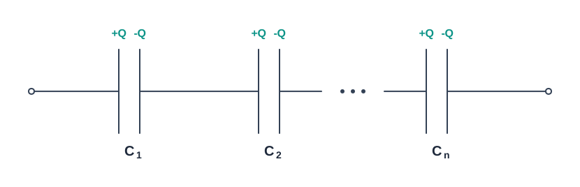
Fig. 2.28 – n capacitors in series.
A useful check: because reciprocals are added, the effective capacitance of a series combination is always smaller than the smallest individual capacitance. Connecting capacitors in series is like stacking their plate separations, which reduces the overall capacitance.
2.14.2 Capacitors in Parallel
Figure 2.29(a) shows two capacitors \(C\_1\) and \(C\_2\) connected in parallel — that is, both wired directly across the same pair of points, so the same potential difference \(V\) is applied across each.
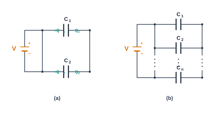
Fig. 2.29 – Capacitors in parallel: (a) two capacitors, (b) n capacitors.
Because the two capacitors generally have different capacitances, the charges they hold need not be equal. Each simply obeys \(Q = CV\) with the common voltage \(V\):
\[Q\_1 = C\_1 V, \\qquad Q\_2 = C\_2 V \\tag{2.61}\]
We now replace the pair by a single equivalent capacitor carrying the total charge:
\[Q = Q\_1 + Q\_2 \\tag{2.62}\]
at the same potential difference \(V\). Therefore:
\[Q = CV = C\_1 V + C\_2 V \\tag{2.63}\]
Cancelling \(V\) gives the rule for two capacitors in parallel:
\[C = C\_1 + C\_2 \\tag{2.64}\]
The same argument extends to any number of capacitors in parallel, as in Fig. 2.29(b). The total charge is the sum of the individual charges:
\[Q = Q\_1 + Q\_2 + \\cdots + Q\_n \\tag{2.65}\]
\[CV = C\_1 V + C\_2 V + \\cdots + C\_n V \\tag{2.66}\]
giving the general parallel formula:
\[C = C\_1 + C\_2 + \\cdots + C\_n \\tag{2.67}\]
Notice the contrast with the series case. In parallel, capacitances simply add, so the effective capacitance is always larger than the largest individual one — connecting capacitors in parallel is like enlarging the total plate area. In series, reciprocals add and the effective capacitance is smaller than the smallest. Keeping these two behaviours straight is essential for solving network problems.
A network of four \(10\\ \\mu\\text{F}\) capacitors is connected to a \(500\\ \\text{V}\) supply, as shown in Fig. 2.30. Determine (a) the equivalent capacitance of the network and (b) the charge on each capacitor. (Note: the charge on a capacitor means the charge on its higher-potential plate, equal and opposite to the charge on its lower-potential plate.)
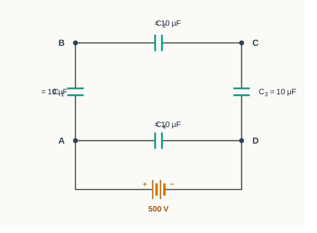
[Caption:] Fig. 2.30 – A network of four capacitors. [/Caption:]
Solution
- In this network, \(C\_1\), \(C\_2\), and \(C\_3\) are connected in series. Their combined capacitance \(C'\) is given by:
\[\\frac{1}{C'} = \\frac{1}{C\_1} + \\frac{1}{C\_2} + \\frac{1}{C\_3}\]
For \(C\_1 = C\_2 = C\_3 = 10\\ \\mu\\text{F}\), this gives \(C' = \\dfrac{10}{3}\\ \\mu\\text{F}\). The network then has \(C'\) and \(C\_4\) connected in parallel, so the equivalent capacitance of the whole network is:
\[C = C' + C\_4 = \\left(\\frac{10}{3} + 10\\right)\\mu\\text{F} = 13.3\\ \\mu\\text{F}\]
- From the figure, the charge on each of \(C\_1\), \(C\_2\), and \(C\_3\) is the same (they are in series); call it \(Q\). Let the charge on \(C\_4\) be \(Q'\). Since the potential difference across AB is \(Q/C\_1\), across BC is \(Q/C\_2\), and across CD is \(Q/C\_3\), their sum equals the supply voltage:
\[\\frac{Q}{C\_1} + \\frac{Q}{C\_2} + \\frac{Q}{C\_3} = 500\\ \\text{V}\]
Also, \(Q'/C\_4 = 500\\ \\text{V}\). Substituting the given capacitances:
\[Q = 500\\ \\text{V} \\times \\frac{10}{3}\\ \\mu\\text{F} = 1.7\\times10^{-3}\\ \\text{C}\]
\[Q' = 500\\ \\text{V} \\times 10\\ \\mu\\text{F} = 5.0\\times10^{-3}\\ \\text{C}\]
2.15 Energy Stored in a Capacitor
A charged capacitor does not just hold charge — it holds energy. That energy was put in while charging the capacitor, and it can be released later. We now calculate exactly how much energy a capacitor stores.
A capacitor is a pair of conductors with charges \(Q\) and \(-Q\). Imagine building this up from scratch: start with two uncharged conductors 1 and 2, and transfer positive charge, bit by bit, from conductor 2 to conductor 1. At the end, conductor 1 has charge \(Q\) and, by charge conservation, conductor 2 has charge \(-Q\), as in Fig. 2.31.
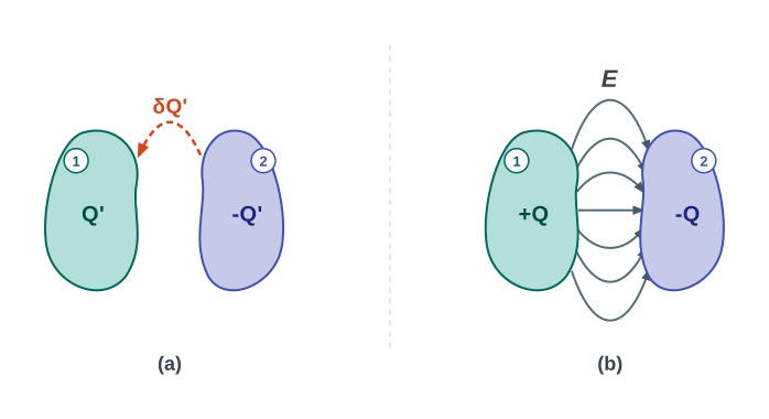
Fig. 2.31 – Charging a capacitor and storing energy in its field.
Adding up the work
Transferring positive charge from conductor 2 to conductor 1 requires work by an external agency, because at every stage conductor 1 is at a higher potential than conductor 2, so the incoming positive charge is pushed uphill in potential.
To find the total work, first look at one small step. Suppose at some intermediate stage the conductors carry charges \(Q'\) and \(-Q'\). The potential difference between them is then \(V' = Q'/C\), where \(C\) is the capacitance. Now transfer a tiny extra charge \(\\delta Q'\) from conductor 2 to conductor 1. The work done in this step, which raises the charge from \(Q'\) to \(Q' + \\delta Q'\), is:
\[\\delta W = V'\\delta Q' = \\frac{Q'}{C}\\delta Q' \\tag{2.68}\]
The total work is the sum of all these little steps as the charge grows from \(0\) to \(Q\), which is an integral:
\[W = \\int\_0^Q \\frac{Q'}{C}\\delta Q' = \\frac{1}{C}\\frac{Q'^2}{2}\\bigg|\_0^Q = \\frac{Q^2}{2C}\]
Using \(Q = CV\), this same result can be written in three equivalent forms:
\[W = \\frac{Q^2}{2C} = \\frac{1}{2}CV^2 = \\frac{1}{2}QV \\tag{2.69}\]
Since the electrostatic force is conservative, this work is stored as the potential energy of the charged capacitor. And because the force is conservative, the result is independent of how the capacitor was charged. When the capacitor later discharges, this stored energy is released.
Energy stored in the field
It is illuminating to view this stored energy as residing in the electric field between the plates, rather than “on” the plates. To see this, take a parallel plate capacitor with plate area \(A\) and separation \(d\). Its stored energy is:
\[\\frac{1}{2}\\frac{Q^2}{C} = \\frac{(A\\sigma)^2}{2}\\times\\frac{d}{\\varepsilon\_0 A} \\tag{2.70}\]
where we used \(Q = A\\sigma\) and \(C = \\varepsilon\_0 A/d\). The surface charge density is related to the field between the plates by:
\[E = \\frac{\\sigma}{\\varepsilon\_0} \\tag{2.71}\]
Substituting Eq. (2.71) into Eq. (2.70), the energy stored takes the compact form:
\[U = \\frac{1}{2}\\varepsilon\_0 E^2 \\times Ad \\tag{2.72}\]
Now \(Ad\) is precisely the volume of the region between the plates — the region where the electric field exists. If we define the energy density as the energy stored per unit volume, Eq. (2.72) shows it to be:
\[u = \\frac{1}{2}\\varepsilon\_0 E^2 \\tag{2.73}\]
Although we derived Eq. (2.73) for the special case of a parallel plate capacitor, the result is in fact completely general: wherever an electric field \(E\) exists, it carries energy of density \(\\frac{1}{2}\\varepsilon\_0 E^2\), regardless of the charge configuration that produced it. This is a powerful idea — energy can be thought of as spread throughout the field itself.
(a) A \(900\\ \\text{pF}\) capacitor is charged by a \(100\\ \\text{V}\) battery [Fig. 2.32(a)]. How much electrostatic energy is stored by the capacitor?
(b) The capacitor is then disconnected from the battery and connected to another (uncharged) \(900\\ \\text{pF}\) capacitor [Fig. 2.32(b)]. What is the electrostatic energy stored by the system now?
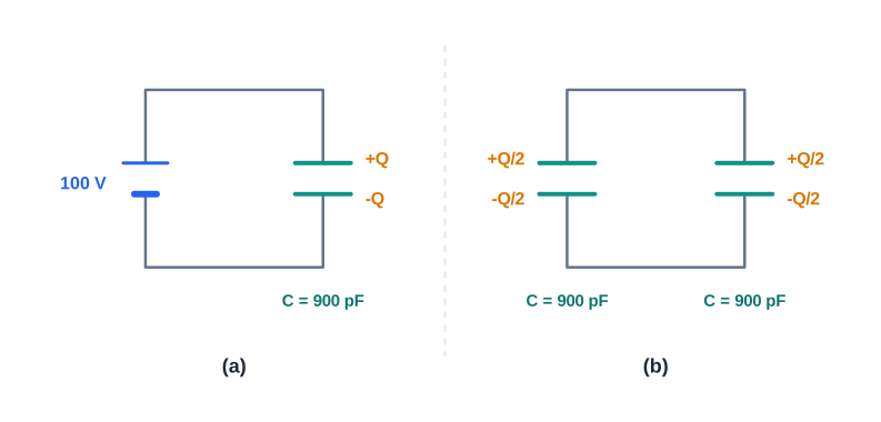
[Caption:] Fig. 2.32 – Sharing charge between two identical capacitors. [/Caption:]
Solution
- The charge on the capacitor is:
\[Q = CV = 900\\times10^{-12}\\ \\text{F}\\times100\\ \\text{V} = 9\\times10^{-8}\\ \\text{C}\]
The energy stored is:
\[= \\frac{1}{2}CV^2 = \\frac{1}{2}QV = \\frac{1}{2}\\times9\\times10^{-8}\\ \\text{C}\\times100\\ \\text{V} = 4.5\\times10^{-6}\\ \\text{J}\]
- In the final steady state, the two capacitors have their positive plates at the same potential and their negative plates at the same potential. Let the common potential difference be \(V'\). The charge on each capacitor is then \(Q' = CV'\). By charge conservation, the original charge is shared equally, so \(Q' = Q/2\), which implies \(V' = V/2\). The total energy of the system is:
\[= 2\\times\\frac{1}{2}Q'V' = \\frac{1}{4}QV = 2.25\\times10^{-6}\\ \\text{J}\]
Thus, in going from (a) to (b), although no charge is lost, the final energy is only half the initial energy. Where has the remaining energy gone? During the brief moment of connection, a transient current flows from the first capacitor to the second, and energy is lost during this time as heat and electromagnetic radiation.
2.16 Summary
- The electrostatic force is a conservative force. The work done by an external force — equal and opposite to the electrostatic force — in bringing a charge \(q\) from a point R to a point P is \(q(V\_P - V\_R)\), which is the difference in the potential energy of the charge \(q\) between the final and initial points.
- The potential at a point is the work done per unit charge (by an external agency) in bringing a charge from infinity to that point. Potential is defined only up to an additive constant, since it is the potential difference between two points that is physically significant. Choosing the potential at infinity to be zero, the potential at a point with position vector \(\\vec{r}\) due to a point charge \(Q\) placed at the origin is: \[V(\\vec{r}) = \\frac{1}{4\\pi\\varepsilon\_0}\\frac{Q}{r}\]
- The electrostatic potential at a point with position vector \(\\vec{r}\) due to a point dipole of dipole moment \(\\vec{p}\) placed at the origin is: \[V(\\vec{r}) = \\frac{1}{4\\pi\\varepsilon\_0}\\frac{\\vec{p}\\cdot\\hat{\\mathbf{r}}}{r^2}\] The result is also true for a real dipole (charges \(-q\) and \(q\) separated by \(2a\)) when \(r \\gg a\).
- For a charge configuration \(q\_1, q\_2, \\ldots, q\_n\) with position vectors \(\\vec{r}*1, \\vec{r}2, \\ldots, \\vec{r}n\), the potential at a point P is given by the superposition principle: \[V = \\frac{1}{4\\pi\\varepsilon\_0}\\left(\\frac{q\_1}{r{1P}} + \\frac{q\_2}{r{2P}} + \\cdots + \\frac{q\_n}{r*{nP}}\\right)\] where \(r\_{1P}\) is the distance between \(q\_1\) and P, and so on.
- An equipotential surface is a surface over which the potential has a constant value. For a point charge, concentric spheres centred on the charge are equipotential surfaces. The electric field \(\\vec{E}\) at a point is perpendicular to the equipotential surface through that point, and points in the direction of the steepest decrease of potential.
- The potential energy stored in a system of charges is the work done (by an external agency) in assembling the charges at their locations. The potential energy of two charges \(q\_1, q\_2\) at \(\\vec{r}*1, \\vec{r}2\) is: \[U = \\frac{1}{4\\pi\\varepsilon\_0}\\frac{q\_1 q\_2}{r{12}}\] where \(r*{12}\) is the distance between \(q\_1\) and \(q\_2\).
- The potential energy of a charge \(q\) in an external potential \(V(\\vec{r})\) is \(qV(\\vec{r})\). The potential energy of a dipole of moment \(\\vec{p}\) in a uniform electric field \(\\vec{E}\) is \(-\\vec{p}\\cdot\\vec{E}\).
- The electrostatic field \(\\vec{E}\) is zero in the interior of a conductor. Just outside the surface of a charged conductor, \(\\vec{E}\) is normal to the surface, given by: \[\\vec{E} = \\frac{\\sigma}{\\varepsilon\_0}\\hat{\\mathbf{n}}\] where \(\\hat{\\mathbf{n}}\) is the unit vector along the outward normal to the surface and \(\\sigma\) is the surface charge density. Charges given to a conductor reside only at its surface. The potential is constant within and on the surface of a conductor. In a cavity within a conductor (with no charges inside the cavity), the electric field is zero.
- A capacitor is a system of two conductors separated by an insulator. Its capacitance is defined by \(C = Q/V\), where \(Q\) and \(-Q\) are the charges on the two conductors and \(V\) is the potential difference between them. \(C\) is determined purely geometrically — by the shapes, sizes, and relative positions of the two conductors. The unit of capacitance is the farad, with \(1\\ \\text{F} = 1\\ \\text{C V}^{-1}\). For a parallel plate capacitor (with vacuum between the plates): \[C = \\varepsilon\_0\\frac{A}{d}\] where \(A\) is the area of each plate and \(d\) the separation between them.
- If the medium between the plates of a capacitor is filled with an insulating substance (a dielectric), the field of the charged plates induces a net dipole moment in the dielectric. This effect, called polarisation, gives rise to a field in the opposite direction. The net field inside the dielectric — and hence the potential difference between the plates — is thereby reduced. Consequently, the capacitance \(C\) increases from its vacuum value \(C\_0\): \[C = KC\_0\] where \(K\) is the dielectric constant of the insulating substance.
- For capacitors in series, the total capacitance \(C\) is given by: \[\\frac{1}{C} = \\frac{1}{C\_1} + \\frac{1}{C\_2} + \\frac{1}{C\_3} + \\cdots\] For capacitors in parallel, the total capacitance \(C\) is: \[C = C\_1 + C\_2 + C\_3 + \\cdots\] where \(C\_1, C\_2, C\_3, \\ldots\) are the individual capacitances.
- The energy \(U\) stored in a capacitor of capacitance \(C\), with charge \(Q\) and voltage \(V\), is: \[U = \\frac{1}{2}QV = \\frac{1}{2}CV^2 = \\frac{1}{2}\\frac{Q^2}{C}\] The electric energy density (energy per unit volume) in a region with electric field is \(\\dfrac{1}{2}\\varepsilon\_0 E^2\).
Table of physical quantities
| Physical quantity | Symbol | Dimensions | Unit | Remark |
|---|---|---|---|---|
| Potential | \(\\phi\) or \(V\) | \(\[\\text{M}^1\\text{L}^2\\text{T}^{-3}\\text{A}^{-1}]\) | V | Potential difference is physically significant |
| Capacitance | \(C\) | \(\[\\text{M}^{-1}\\text{L}^{-2}\\text{T}^{4}\\text{A}^{2}]\) | F | |
| Polarisation | \(\\vec{P}\) | \(\[\\text{L}^{-2}\\text{AT}]\) | C m⁻² | Dipole moment per unit volume |
| Dielectric constant | \(K\) | Dimensionless | — |
2.17 Points to Ponder
- Electrostatics deals with forces between charges at rest. But if there is a force on a charge, how can it stay at rest? The resolution is that when we speak of electrostatic force between charges, each charge is understood to be held at rest by some other, unspecified force that opposes the net Coulomb force on it.
- A capacitor is built so as to confine the electric field lines within a small region of space. Because of this, even when the field between the plates is quite strong, the potential difference between the two conductors can be small.
- The electric field is discontinuous across the surface of a spherical charged shell: it is zero inside and \(\\dfrac{\\sigma}{\\varepsilon\_0}\\hat{\\mathbf{n}}\) just outside. The electric potential, however, is continuous across the surface, equal to \(\\dfrac{q}{4\\pi\\varepsilon\_0 R}\) at the surface.
- The torque \(\\vec{p}\\times\\vec{E}\) on a dipole tends to make it oscillate about the field direction \(\\vec{E}\). Only if there is a dissipative (energy-losing) mechanism do these oscillations get damped, so that the dipole eventually settles down aligned with \(\\vec{E}\).
- The potential due to a charge \(q\) at its own location is not defined — it is infinite.
- In the expression \(qV(\\vec{r})\) for the potential energy of a charge \(q\), the quantity \(V(\\vec{r})\) is the potential due to external charges, and not the potential due to \(q\) itself. As noted in point 5, this expression would be ill-defined if \(V(\\vec{r})\) were to include the potential due to the charge \(q\) itself.
- A cavity inside a conductor is shielded from outside electrical influences. It is worth noting that electrostatic shielding does not work the other way round: if you place charges inside the cavity, the exterior of the conductor is not shielded from the fields of those inside charges.
2.18 NCERT Questions
- Two charges \(5\\times10^{-8}\\ \\text{C}\) and \(-3\\times10^{-8}\\ \\text{C}\) are located \(16\\ \\text{cm}\) apart. At what point(s) on the line joining the two charges is the electric potential zero? Take the potential at infinity to be zero.
- A regular hexagon of side \(10\\ \\text{cm}\) has a charge \(5\\ \\mu\\text{C}\) at each of its vertices. Calculate the potential at the centre of the hexagon.
- Two charges \(2\\ \\mu\\text{C}\) and \(-2\\ \\mu\\text{C}\) are placed at points A and B, \(6\\ \\text{cm}\) apart.
- Identify an equipotential surface of the system.
- What is the direction of the electric field at every point on this surface?
- A spherical conductor of radius \(12\\ \\text{cm}\) has a charge of \(1.6\\times10^{-7}\\ \\text{C}\) distributed uniformly on its surface. What is the electric field
- inside the sphere,
- just outside the sphere,
- at a point \(18\\ \\text{cm}\) from the centre of the sphere?
- A parallel plate capacitor with air between the plates has a capacitance of \(8\\ \\text{pF}\) (\(1\\ \\text{pF} = 10^{-12}\\ \\text{F}\)). What will be the capacitance if the distance between the plates is reduced by half, and the space between them is filled with a substance of dielectric constant \(6\)?
- Three capacitors each of capacitance \(9\\ \\text{pF}\) are connected in series.
- What is the total capacitance of the combination?
- What is the potential difference across each capacitor if the combination is connected to a \(120\\ \\text{V}\) supply?
- Three capacitors of capacitances \(2\\ \\text{pF}\), \(3\\ \\text{pF}\), and \(4\\ \\text{pF}\) are connected in parallel.
- What is the total capacitance of the combination?
- Determine the charge on each capacitor if the combination is connected to a \(100\\ \\text{V}\) supply.
- In a parallel plate capacitor with air between the plates, each plate has an area of \(6\\times10^{-3}\\ \\text{m}^2\) and the distance between the plates is \(3\\ \\text{mm}\). Calculate the capacitance of the capacitor. If this capacitor is connected to a \(100\\ \\text{V}\) supply, what is the charge on each plate of the capacitor?
- Explain what would happen if, in the capacitor given in Question 8, a \(3\\ \\text{mm}\) thick mica sheet (of dielectric constant \(6\)) were inserted between the plates,
- while the voltage supply remained connected,
- after the supply was disconnected.
- A \(12\\ \\text{pF}\) capacitor is connected to a \(50\\ \\text{V}\) battery. How much electrostatic energy is stored in the capacitor?
- A \(600\\ \\text{pF}\) capacitor is charged by a \(200\\ \\text{V}\) supply. It is then disconnected from the supply and connected to another uncharged \(600\\ \\text{pF}\) capacitor. How much electrostatic energy is lost in the process?
2.19 Check Your Concepts
- Electric potential is a scalar quantity, whereas the electric field is a vector. Explain how this difference makes the calculation of the potential due to a system of many charges simpler than the calculation of the field.
- The potential due to a single point charge falls off as \(1/r\), but the potential due to a dipole falls off as \(1/r^2\). Explain physically why the dipole’s potential decreases more rapidly with distance.
- State whether the following is true and justify it: “In the static situation, the electric field inside a conductor is zero, and therefore the entire conductor — interior and surface — is at one constant potential.” Explain the reasoning that links the two statements.
- A test charge is moved from one point to another along an equipotential surface, and then along a path that crosses several equipotential surfaces. In which case is work done, and why? Relate your answer to the angle between the electric field and the equipotential surface.
- Explain why the effective capacitance of capacitors joined in series is always smaller than the smallest of them, while that of capacitors joined in parallel is always larger than the largest.
- An isolated parallel plate capacitor is charged and then disconnected from the battery. A dielectric slab is now inserted, completely filling the gap. State and explain what happens to (i) the charge, (ii) the capacitance, (iii) the potential difference, and (iv) the energy stored.
- A dipole is placed in a uniform external electric field. Explain why it experiences a torque but no net force, and identify the orientations of stable and unstable equilibrium in terms of its potential energy \(U = -\\vec{p}\\cdot\\vec{E}\).
- Why is the electric field just outside the surface of a charged conductor equal to \(\\sigma/\\varepsilon\_0\), whereas the field due to an isolated infinite charged sheet is only \(\\sigma/2\\varepsilon\_0\)? Account for the factor of two.
2.20 Practice with Numericals
- Calculate the electric potential at a point \(3\\ \\text{cm}\) away from an isolated point charge of \(2\\times10^{-9}\\ \\text{C}\). (Take \(\\dfrac{1}{4\\pi\\varepsilon\_0} = 9\\times10^{9}\\ \\text{N m}^2,\\text{C}^{-2}\).)
- A short electric dipole of dipole moment \(4\\times10^{-30}\\ \\text{C m}\) is placed in vacuum. Find the electric potential at a point \(2\\ \\text{nm}\) from its centre, lying on the axis of the dipole. (Take \(\\dfrac{1}{4\\pi\\varepsilon\_0} = 9\\times10^{9}\\ \\text{N m}^2,\\text{C}^{-2}\).)
- An external agent carries a charge of \(+3\\ \\mu\\text{C}\), without acceleration, from a point at potential \(40\\ \\text{V}\) to a point at potential \(160\\ \\text{V}\). Calculate the work done.
- Three point charges \(+1\\ \\mu\\text{C}\), \(+2\\ \\mu\\text{C}\), and \(-3\\ \\mu\\text{C}\) are placed at the corners of an equilateral triangle of side \(10\\ \\text{cm}\). Find the total electrostatic potential energy of the system. (Take \(\\dfrac{1}{4\\pi\\varepsilon\_0} = 9\\times10^{9}\\ \\text{N m}^2,\\text{C}^{-2}\).)
- In a certain region the electric field is uniform. The potential falls steadily by \(150\\ \\text{V}\) over a distance of \(5\\ \\text{cm}\) measured along the field. Find the magnitude of the electric field.
- A parallel plate capacitor has plates each of area \(200\\ \\text{cm}^2\) separated by \(1\\ \\text{mm}\). The gap between the plates is completely filled with a dielectric of dielectric constant \(5\). Calculate the capacitance. (Take \(\\varepsilon\_0 = 8.85\\times10^{-12}\\ \\text{C}^2,\\text{N}^{-1},\\text{m}^{-2}\).)
- Two capacitors of \(4\\ \\mu\\text{F}\) and \(12\\ \\mu\\text{F}\) are first connected in series, and then the series combination is connected in parallel with a third capacitor of \(6\\ \\mu\\text{F}\). Find the equivalent capacitance of the whole arrangement.
- A \(50\\ \\mu\\text{F}\) capacitor is charged to a potential difference of \(200\\ \\text{V}\). Calculate (i) the charge stored, (ii) the energy stored in the capacitor.