Chapter 4: Moving Charges and Magnetism
In the summer of 1820, the Danish physicist Hans Christian Oersted was giving a lecture demonstration to his students in Copenhagen. A wire carrying current lay on the table, and a small magnetic compass happened to be placed near it. As Oersted switched the current on, something odd caught his eye: the compass needle twitched and swung away from its usual north-south direction. At first, this seemed like a minor disturbance, easy to dismiss. But Oersted did not dismiss it. He repeated the experiment, moved the compass closer and farther, reversed the direction of the current, and sprinkled iron filings around the wire to map out what was happening in the space around it. Each time, the pattern was consistent and unmistakable: electricity, all on its own, was creating a magnetic effect in the surrounding space.
For centuries, electricity and magnetism had been studied as two separate, unrelated subjects. Oersted’s simple classroom accident shattered that separation and opened the door to one of the great unifications in physics.
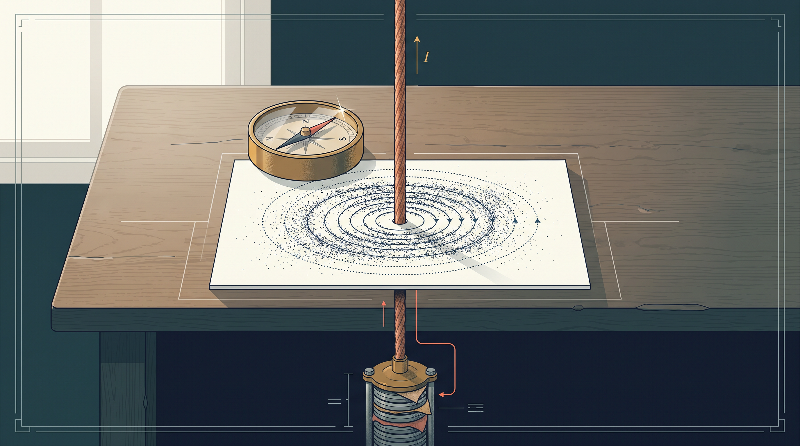
Fig. 4.0 – Oersted’s compass demonstration.
This chapter will help you answer all of these questions.
4.1 Introduction
Electricity and magnetism have each been known to humankind for more than 2000 years. Ancient civilisations knew that rubbing certain materials produced electric effects, and that certain stones (natural magnets) could attract iron. For most of this long history, however, these two effects were treated as completely separate branches of science, with no known connection between them.
That view changed dramatically about 200 years ago, in 1820. During a lecture demonstration, the Danish physicist Hans Christian Oersted noticed something unexpected: a compass needle, placed near a wire, twitched and turned whenever current flowed through that wire. This simple, almost accidental observation turned out to be one of the most important discoveries in the history of physics, because it showed for the first time that electricity and magnetism are not independent phenomena at all — they are deeply connected.
Oersted did not stop at the first observation. He investigated the effect carefully and found a clear pattern. When a straight wire carries a current, a compass needle placed near it lines up tangentially — that is, along the edge — of an imaginary circle. This circle has the wire passing through its centre, and its plane is perpendicular to the wire, as shown in Fig. 4.1(a).
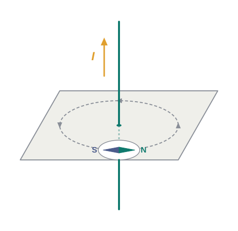
Fig. 4.1(a) – Compass needle deflected by a current.
This effect is easiest to see when the current in the wire is large and the compass needle is placed close to the wire. Under these conditions, the magnetic effect of the current dominates over the Earth’s own (much weaker) magnetic field, so the Earth’s field can be safely ignored while observing the deflection.
Oersted also discovered that reversing the direction of current flow reverses the direction in which the needle points, as shown in Fig. 4.1(b). This tells us that the magnetic effect has a definite direction associated with the current — it is not a simple, direction-less push.
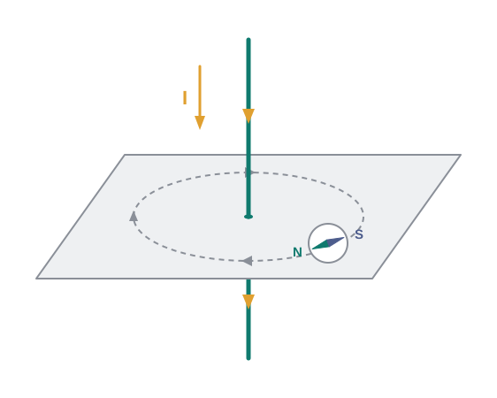
Fig. 4.1(b) – Deflection reverses with current direction.
Two more features complete the picture. First, the deflection of the needle becomes larger if the current is increased, or if the needle is brought closer to the wire. Second, if iron filings are sprinkled on a flat surface around the wire (with the wire passing through perpendicular to that surface), the filings arrange themselves in a striking pattern: concentric circles, all centred on the wire, as shown in Fig. 4.1(c).
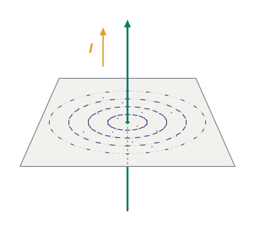
Fig. 4.1(c) – Magnetic field lines traced by iron filings.
Putting all these observations together, Oersted arrived at a conclusion that would reshape physics.
This single sentence is the seed from which the entire subject of electromagnetism grew. Before Oersted, “electric” effects and “magnetic” effects were studied by different scientists using different instruments and different ideas. After Oersted, physicists began to search for a deeper, unified description that could explain both effects using the same underlying principles.
That search moved quickly. By 1864, the Scottish physicist James Clerk Maxwell had unified the laws of electricity and magnetism into a single, elegant mathematical framework. As a striking consequence of this unification, Maxwell realised that light itself is an electromagnetic wave — a travelling disturbance of electric and magnetic fields.
The 20th century then saw remarkable scientific and technological progress, built directly on this improved understanding of electromagnetism. This progress made possible the invention of devices that could produce, amplify, transmit, and detect electromagnetic waves — technologies that now underpin radio, television, mobile communication, and much more.
This chapter builds on that foundation. We shall see how a magnetic field exerts forces on moving charged particles, such as electrons and protons, and on current-carrying wires. We shall also learn, in more detail than Oersted could have known in 1820, exactly how currents produce magnetic fields. Finally, we shall study how currents and voltages in a circuit can be measured using a device called a galvanometer, which works because of the very effect Oersted first noticed.
Before going further, it is useful to fix a convention that will be used throughout this chapter and the next. A current or a magnetic field that emerges out of the plane of the page is represented by a dot (\(\\odot\)). A current or a magnetic field that goes into the plane of the page is represented by a cross (\(\\otimes\)). You can think of the dot as the tip of an arrow pointing towards you, and the cross as the tail feathers of an arrow moving away from you. Figures 4.1(a) and 4.1(b) above correspond to these two situations, respectively.
4.2 Magnetic Force
4.2.1 Sources and fields
Before we introduce the idea of a magnetic field, it helps to recall what you already know about the electric field from Chapter 1. There, the interaction between two charges was understood as a two-step process. First, a charge \(Q\), acting as the source, produces an electric field \(\\vec{E}\) at every point in the surrounding space. This field is given by
\[\\vec{E} = \\frac{Q, \\hat{r}}{4\\pi\\varepsilon\_0, r^2} \\tag{4.1}\]
Here, \(\\hat{r}\) is the unit vector pointing along the direction of \(\\vec{r}\) (the position vector from the source charge to the point where the field is being calculated), \(\\varepsilon\_0\) is the permittivity of free space, and \(r\) is the distance from \(Q\) to that point. Being a vector field, \(\\vec{E}\) has both a magnitude and a direction defined at every point in space.
In the second step, any other charge \(q\) placed in this field experiences a force \(\\vec{F}\), given by
\[\\vec{F} = q\\vec{E} = \\frac{qQ, \\hat{r}}{4\\pi\\varepsilon\_0, r^2} \\tag{4.2}\]
As emphasised in Chapter 1, the field \(\\vec{E}\) is not merely a bookkeeping device to calculate forces — it has genuine physical existence. It can carry energy and momentum from one place to another, and it is not established instantaneously; a change in the source takes a finite time to propagate outward through the field. This idea of a field as a real, physical entity was strongly championed by Michael Faraday, and it was later given precise mathematical form by Maxwell when he unified electricity and magnetism.
An electric field can, in general, depend on time as well as on position. In this chapter, however, we will restrict our attention to situations where the fields do not change with time, which considerably simplifies the discussion.
When more than one charge is present, the resultant field at any point is simply the vector sum of the fields due to each individual charge. You already met this idea in Chapter 1 as the principle of superposition. Once the total field at a point is known, the force on any test charge placed there follows directly from Eq. (4.2).
Just as static (stationary) charges produce an electric field, moving charges — that is, currents — produce, in addition, a magnetic field, denoted \(\\vec{B}(\\vec{r})\). This is again a vector field: it has a definite magnitude and direction at every point in space, and in general it may also depend on time. The magnetic field shares an important property with the electric field: it too obeys the principle of superposition.
4.2.2 Magnetic Field, Lorentz Force
Consider a point charge \(q\), moving with velocity \(\\vec{v}\), located at position \(\\vec{r}\) at some instant of time \(t\). Suppose this charge is present in a region where both an electric field \(\\vec{E}(\\vec{r})\) and a magnetic field \(\\vec{B}(\\vec{r})\) exist simultaneously. The total force experienced by the charge due to both fields together can be written as
\[\\vec{F} = q\\left\[\\vec{E}(\\vec{r}) + \\vec{v} \\times \\vec{B}(\\vec{r})\\right] \\equiv \\vec{F}*{\\text{electric}} + \\vec{F}*{\\text{magnetic}} \\tag{4.3}\]
This total force is called the Lorentz force, named after the Dutch physicist H.A. Lorentz, who first wrote it down based on extensive experimental work carried out earlier by Ampere and others.
You have already studied the electric part of this force, \(q\\vec{E}\), in detail in earlier chapters. Let us now focus on the magnetic part, \(q(\\vec{v} \\times \\vec{B})\), and examine its key features one by one.
(i) It depends on \(q\), \(\\vec{v}\), and \(\\vec{B}\). The magnetic force depends jointly on the charge of the particle, its velocity, and the magnetic field it moves through. An important consequence is that the force on a negative charge is exactly opposite in direction to the force on a positive charge moving in the same way through the same field.
(ii) It involves a vector (cross) product. The term \(\\vec{v} \\times \\vec{B}\) is a vector product of the velocity and the magnetic field. Recall from your study of vectors that the cross product of two vectors is zero whenever those vectors are parallel or anti-parallel to each other. This has a direct physical meaning here: the magnetic force vanishes whenever the charged particle moves exactly along the direction of the magnetic field (or exactly opposite to it). When the force is non-zero, it acts in a sideways direction — perpendicular to both the velocity and the magnetic field at once. The exact direction is given by the right-hand rule (or equivalently, the screw rule) for vector products, illustrated in Fig. 4.2.
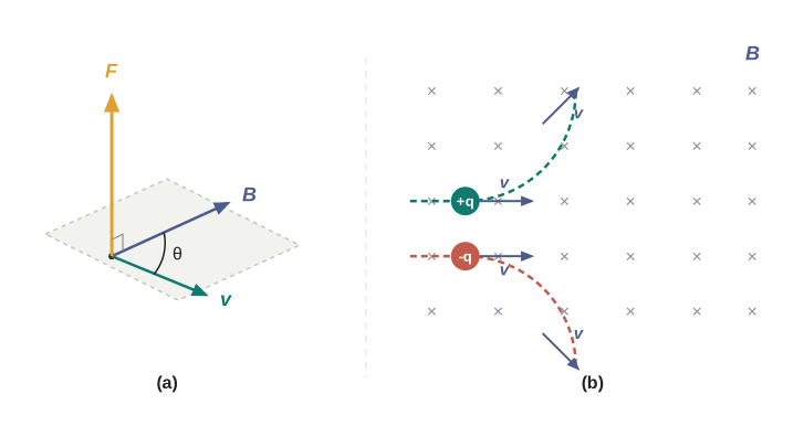
Fig. 4.2 – Magnetic force on a moving charge: (a) right-hand rule and (b) opposite deflections.
(iii) A stationary charge feels no magnetic force. Since the magnetic force depends on \(\\vec{v}\), if the charge is not moving at all (so \(|\\vec{v}| = 0\)), there is simply no magnetic force on it. Only a moving charge experiences a magnetic force — this is one of the most fundamental distinctions between electric and magnetic forces.
Defining the unit of magnetic field. The expression for the magnetic force also gives us a natural way to define the magnitude of the magnetic field itself. If we take \(q\), \(F\), and \(v\) all equal to one (in SI units) in the force equation
\[\\vec{F} = q(\\vec{v} \\times \\vec{B}) = qvB\\sin\\theta, \\hat{n}\]
(where \(\\theta\) is the angle between \(\\vec{v}\) and \(\\vec{B}\), as shown in Fig. 4.2(a)), we arrive at a working definition: the magnitude of the magnetic field \(B\) is 1 SI unit when a unit charge (1 C), moving perpendicular to \(\\vec{B}\) with a speed of 1 m/s, experiences a force of exactly one newton.
Working out the dimensions, we get \(\[B] = \[F/qv]\), and the corresponding SI unit works out to be newton-second per (coulomb-metre). This unit is given the special name tesla (T), after the engineer and inventor Nikola Tesla (1856–1943). The tesla turns out to be a rather large unit for many everyday situations, so a smaller, non-SI unit called the gauss is also commonly used, where 1 gauss \(= 10^{-4}\) tesla. For comparison, the Earth’s own magnetic field at its surface is only about \(3.6 \\times 10^{-5}\) T — a small fraction of a single tesla.
4.2.3 Magnetic force on a current-carrying conductor
The idea of a magnetic force on a single moving charge can be extended quite naturally to a current-carrying conductor, since a current is, after all, simply a large number of moving charges travelling together.
Consider a straight rod of uniform cross-sectional area \(A\) and length \(l\), carrying mobile charge carriers — think of these as the free electrons in a typical conductor, as discussed in Chapter 3. Let the number density of these mobile carriers (the number of carriers per unit volume) be \(n\). Then the total number of mobile charge carriers contained in the entire rod is \(nlA\).
For a steady current \(I\) flowing through this rod, we may treat each mobile carrier as moving with an average drift velocity \(\\vec{v}\_d\) (recall this idea of drift velocity from Chapter 3). If the rod sits in an external magnetic field \(\\vec{B}\), then the magnetic force on all these carriers together is
\[\\vec{F} = (nlA),q,\\vec{v}\_d \\times \\vec{B}\]
where \(q\) is the charge on a single carrier. Now, recall that the product \(nq\\vec{v}\_d\) is exactly the current density \(\\vec{j}\), and the magnitude \(|(nq\\vec{v}\_d)|,A\) is simply the current \(I\) (see Chapter 3 for a fuller discussion of current and current density). Using this, we can rewrite the force as
\[\\vec{F} = \\left\[(nq\\vec{v}\_d),lA\\right]\\times\\vec{B} = \\left\[\\vec{j}Al\\right]\\times\\vec{B} = I\\vec{l}\\times\\vec{B} \\tag{4.4}\]
Here, \(\\vec{l}\) is a vector whose magnitude equals \(l\), the length of the rod, and whose direction is identical to the direction of current flow \(I\). It is worth pausing on one subtlety here: the current \(I\) itself is not a vector quantity — only the length vector \(\\vec{l}\), whose direction we choose to align with the current, is a vector. In going from \(\\vec{j}Al\) to \(I\\vec{l}\), we have essentially transferred the “vector-ness” from the current density \(\\vec{j}\) onto the length \(\\vec{l}\).
Equation (4.4) holds for a straight rod carrying current in a uniform field. It is important to be clear about what \(\\vec{B}\) means here: it is the external magnetic field in which the rod is placed — not the magnetic field that the rod’s own current produces. These are two entirely different fields, and it is easy to confuse them if you are not careful.
What if the wire is not straight, but bent into some arbitrary shape? In that case, we can still find the total force by treating the wire as a large collection of tiny straight segments, each of length \(d\\vec{l}\_j\), calculating the force on each tiny segment, and then summing over all of them:
\[\\vec{F} = \\sum\_j I, d\\vec{l}\_j \\times \\vec{B}\]
In most practical cases, this summation over infinitesimally small segments is converted into an integral, which can then be evaluated using the tools of calculus.
A straight wire of mass 200 g and length 1.5 m carries a current of 2 A. It is suspended in mid-air, held up entirely by a uniform horizontal magnetic field \(\\vec{B}\) (Fig. 4.3). What is the magnitude of this magnetic field?
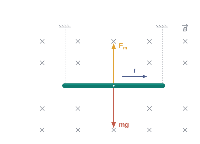
[Caption:] Fig. 4.3 – Equilibrium of a suspended current-carrying wire. [/Caption:]
From Eq. (4.4), the magnetic force on the wire has an upward magnitude \(IlB\) (using the fact that the wire, current, and field are mutually perpendicular here, so \(\\sin\\theta = 1\)). Since the wire is suspended — that is, in equilibrium — this upward magnetic force must exactly balance the downward force of gravity on the wire:
\[mg = IlB\]
\[B = \\frac{mg}{Il} = \\frac{0.2 \\times 9.8}{2 \\times 1.5} = 0.65\\ \\text{T}\]
It is worth noting that it would have been enough to be given just \(m/l\), the mass per unit length of the wire, rather than the mass and length separately. Also notice that the Earth’s magnetic field, roughly \(4 \\times 10^{-5}\) T, is more than four orders of magnitude smaller than the 0.65 T field found here, which is why it has been safely neglected in this calculation.
Suppose the magnetic field points along the positive \(y\)-axis, and a charged particle moves along the positive \(x\)-axis (Fig. 4.4). In which direction does the Lorentz force act on (a) an electron (a negative charge), and (b) a proton (a positive charge)?
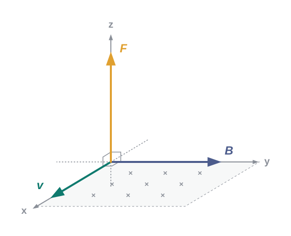
[Caption:] Fig. 4.4 – Directions of velocity, magnetic field, and Lorentz force. [/Caption:]
The velocity \(\\vec{v}\) of the particle points along the \(x\)-axis, while the field \(\\vec{B}\) points along the \(y\)-axis. Using the right-hand (screw) rule for the cross product, \(\\vec{v}\\times\\vec{B}\) points along the \(z\)-axis. Since the force on a positive charge is \(q(\\vec{v}\\times\\vec{B})\) and the force on a negative charge is opposite to this:
For the electron (negative charge), the force acts along the \(-z\) axis.
For the proton (positive charge), the force acts along the \(+z\) axis.
This example is a direct illustration of feature (i) discussed above: for identical velocity and field directions, oppositely charged particles feel oppositely directed magnetic forces.
4.3 Motion in a Magnetic Field
We now look more closely at how a charged particle moves once it is inside a magnetic field. To understand this properly, it helps to first recall an idea from mechanics (Class XI): a force does work on a particle only if that force has some component along — or opposite to — the direction in which the particle is moving. If the force is always exactly perpendicular to the motion, it does no work at all.
This is precisely the situation for the magnetic force. Since the magnetic force on a moving charge, \(q(\\vec{v}\\times\\vec{B})\), is always perpendicular to the particle’s velocity \(\\vec{v}\), it can never do any work on the particle. As a direct consequence, the magnetic force can never change the speed (that is, the magnitude of the velocity) of a charged particle — although it can and does change the direction of the particle’s momentum, bending its path.
This behaviour is quite different from that of an electric field. The electric force on a charge, \(q\\vec{E}\), can have a component parallel (or anti-parallel) to the particle’s velocity, and so it can transfer energy to the particle, speeding it up or slowing it down, in addition to changing its momentum.
Case 1: velocity perpendicular to the field. Let us now consider a charged particle moving through a uniform magnetic field, and first take the simplest case where the velocity \(\\vec{v}\) is exactly perpendicular to \(\\vec{B}\). Here, the perpendicular magnetic force \(q\\vec{v}\\times\\vec{B}\) plays the role of a centripetal force — a force that is always directed towards a fixed centre, keeping the particle moving in a circle. Because \(\\vec{v}\) and \(\\vec{B}\) are perpendicular to each other throughout, the particle traces out a perfect circle, as shown in Fig. 4.5.
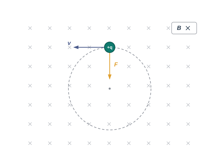
Fig. 4.5 – Circular motion of a charge in a perpendicular uniform magnetic field.
Case 2: velocity has a component along the field. Now suppose the velocity has some component directed along \(\\vec{B}\) as well. This component along the field direction is completely unaffected by the magnetic field (since a magnetic field cannot exert a force on motion parallel to itself, as we saw in Section 4.2). Meanwhile, the component of velocity perpendicular to \(\\vec{B}\) still produces circular motion exactly as before. Putting these two motions together — uniform circular motion in the plane perpendicular to \(\\vec{B}\), combined with uniform straight-line motion along \(\\vec{B}\) — produces a spiralling path called helical motion, illustrated in Fig. 4.6.
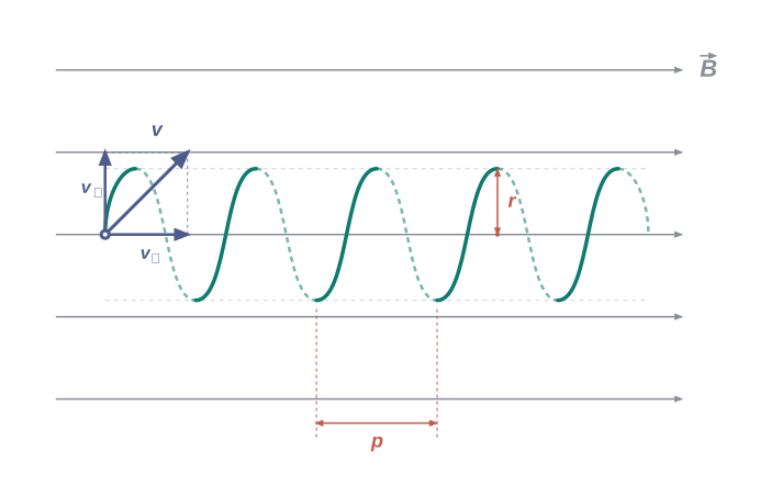
Fig. 4.6 – Helical path of a charged particle in a uniform magnetic field.
Finding the radius of the circular path. You have already learnt, in earlier classes, that if a particle moves in a circle of radius \(r\), a force of magnitude \(mv^2/r\) must act on it, directed towards the centre of the circle — this is called the centripetal force. When the velocity \(v\) is perpendicular to the magnetic field \(B\), the magnetic force itself supplies this centripetal force, and has magnitude \(qvB\). Equating the two expressions for the required centripetal force:
\[\\frac{mv^2}{r} = qvB\]
which, on simplifying, gives the radius of the circular path:
\[r = \\frac{mv}{qB} \\tag{4.5}\]
This result tells us something intuitive: the larger the particle’s momentum \(mv\), the larger the radius of the circle it traces — a particle with more momentum resists being bent into a tight curve, so it sweeps out a bigger circle.
If \(\\omega\) is the angular frequency of this circular motion, then the usual relation between linear speed and angular frequency, \(v = \\omega r\), lets us rewrite Eq. (4.5) as
\[\\omega = 2\\pi\\nu = \\frac{qB}{m} \\tag{4.6(a)}\]
Here, \(\\nu\) (the Greek letter nu) is the frequency of rotation — the number of complete circles the particle traces per second.
A remarkable feature of Eq. [4.6(a)] is that the frequency \(\\nu\) does not depend on the particle’s velocity or its kinetic energy at all — it depends only on the charge \(q\), the field \(B\), and the mass \(m\). In other words, whether the particle is moving fast or slow, it takes exactly the same time to complete one revolution, provided \(q\), \(B\), and \(m\) stay the same.
The time taken for the particle to complete one full revolution is called the period, \(T = 2\\pi/\\omega \\equiv 1/\\nu\).
If the particle’s velocity has a component parallel to the magnetic field, denoted \(v\_{\\parallel}\), this component (as discussed above) makes the particle drift steadily along the direction of the field while it simultaneously circles around, producing the helical path shown in Fig. 4.6. The distance the particle moves along the magnetic field direction during one complete revolution is called the pitch, \(p\), of the helix. Using Eq. [4.6(a)], the pitch works out to be
\[p = v\_{\\parallel} T = \\frac{2\\pi m v\_{\\parallel}}{qB} \\tag{4.6(b)}\]
The radius of the circular part of this helical motion is simply called the radius of the helix, and is still given by Eq. (4.5), using only the perpendicular component of velocity.
4.4 Magnetic Field due to a Current Element, Biot-Savart Law
All the magnetic fields we encounter in nature arise either from currents (that is, from moving charges) or from the intrinsic magnetic moments carried by individual particles. In this section, we focus on the first of these: how exactly does a current produce a magnetic field at some point in space? The precise relationship between a current and the field it creates is given by the Biot-Savart law.
Fig. 4.7 shows a finite conductor \(XY\) carrying a steady current \(I\). Imagine breaking this conductor up into infinitesimally small pieces, and consider one such tiny element, of length \(d\\vec{l}\). We want to find the magnetic field \(d\\vec{B}\) that this one small element produces at some point P, located at a distance \(r\) from it. Let \(\\theta\) be the angle between the direction of the current element \(d\\vec{l}\) and the displacement vector \(\\vec{r}\) that points from the element to P.
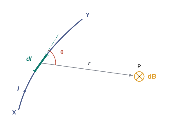
Fig. 4.7 – Magnetic field produced by a current element.
According to the Biot-Savart law, the magnitude of this small field \(d\\vec{B}\) depends on three things: it is directly proportional to the current \(I\), directly proportional to the length of the element \(|d\\vec{l}|\), and inversely proportional to the square of the distance \(r\) from the element to the point P. Its direction is perpendicular to the plane that contains both \(d\\vec{l}\) and \(\\vec{r}\). Putting all of this together in vector notation,
\[d\\vec{B} \\propto \\frac{I,d\\vec{l}\\times \\vec{r}}{r^3} = \\frac{\\mu\_0}{4\\pi}, \\frac{I,d\\vec{l}\\times \\vec{r}}{r^3} \\tag{4.7(a)}\]
where \(\\mu\_0/4\\pi\) is simply the constant of proportionality that makes the units work out correctly in SI units. This expression holds when the current element sits in vacuum (or, to an excellent approximation, in air).
Taking the magnitude of both sides of Eq. [4.7(a)], and using the standard property of the cross product (that \(|\\vec{A}\\times\\vec{B}| = AB\\sin\\theta\)), we get the scalar version of the Biot-Savart law:
\[|d\\vec{B}| = \\frac{\\mu\_0}{4\\pi}, \\frac{I,dl\\sin\\theta}{r^2} \\tag{4.7(b)}\]
Equation [4.7(a)] is the fundamental relation for magnetic fields produced by currents — much as Coulomb’s law was the fundamental relation for electric fields produced by charges. The proportionality constant \(\\mu\_0/4\\pi\) has an exact, fixed value in SI units:
\[\\frac{\\mu\_0}{4\\pi} = 10^{-7}\\ \\text{T m/A} \\tag{4.7(c)}\]
The constant \(\\mu\_0\) itself is called the permeability of free space (or of vacuum).
To find the total magnetic field at point P due to the entire conductor (not just one small element), we must add up — that is, integrate — this vector expression over the whole length of the conductor.
Comparing the Biot-Savart law with Coulomb’s law. It is instructive to compare this new law for the magnetic field with the electrostatic Coulomb’s law you already know, since the two share some features but differ sharply in others.
Both laws are long range: both fall off as the inverse square of the distance from the source to the point of interest, and the principle of superposition applies to both fields. In this connection, it is worth noting that the magnetic field is linear in its source \(I,d\\vec{l}\), in exactly the same way that the electrostatic field is linear in its source, the electric charge.
The electrostatic field is produced by a scalar source — the electric charge, which has no direction of its own. The magnetic field, by contrast, is produced by a vector source, \(I,d\\vec{l}\), which does have a direction (the direction of current flow).
The electrostatic field points along the displacement vector joining the source charge to the field point. The magnetic field, however, is perpendicular to the plane containing the displacement vector \(\\vec{r}\) and the current element \(I,d\\vec{l}\) — a completely different geometric relationship.
There is an angular dependence in the Biot-Savart law that has no counterpart in the electrostatic case. Looking again at Fig. 4.7, notice that at any point lying exactly along the direction of \(d\\vec{l}\) itself (the dashed line in the figure), the magnetic field is zero. Along this line, \(\\theta = 0\), so \(\\sin\\theta = 0\), and from Eq. [4.7(a)], \(|d\\vec{B}| = 0\).
There is also an interesting and important relationship connecting three fundamental constants: \(\\varepsilon\_0\), the permittivity of free space; \(\\mu\_0\), the permeability of free space; and \(c\), the speed of light in vacuum:
\[\\varepsilon\_0\\mu\_0 = (4\\pi\\varepsilon\_0)\\frac{\\mu\_0}{4\\pi} = \\frac{1}{9\\times10^9}\\left(10^{-7}\\right) = \\frac{1}{(3\\times10^8)^2} = \\frac{1}{c^2}\]
This deep connection between electric and magnetic constants and the speed of light will be explored further in Chapter 8, on electromagnetic waves. Since the speed of light in vacuum is a fixed, unchanging constant, the product \(\\mu\_0\\varepsilon\_0\) must also be fixed in magnitude. This means that once we choose a value for either \(\\varepsilon\_0\) or \(\\mu\_0\), the value of the other is automatically fixed. By convention, in SI units, \(\\mu\_0\) is fixed to be exactly \(4\\pi\\times10^{-7}\) in magnitude.
An element \(\\Delta\\vec{l} = \\Delta x,\\hat{i}\) is placed at the origin and carries a large current \(I = 10\) A (Fig. 4.8). What is the magnetic field it produces on the \(y\)-axis, at a distance of 0.5 m, given \(\\Delta x = 1\) cm?
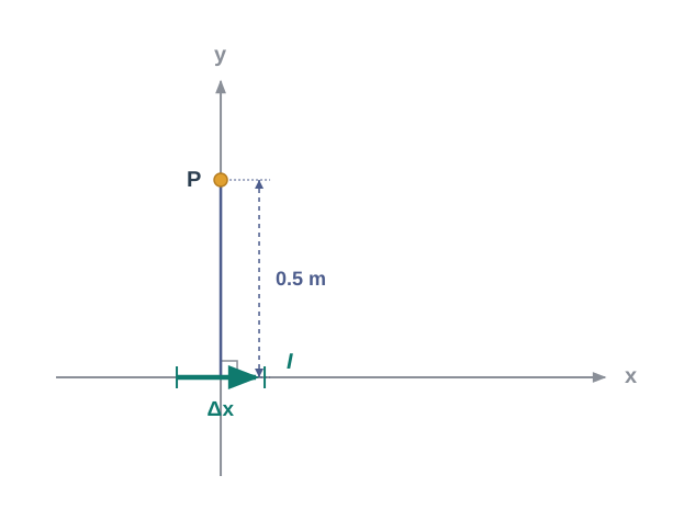
[Caption:] Fig. 4.8 – Magnetic field of a current element at the origin. [/Caption:]
Using Eq. (4.7), \(|d\\vec{B}| = \\dfrac{\\mu\_0}{4\\pi},\\dfrac{I,dl\\sin\\theta}{r^2}\)
Here, \(dl = \\Delta x = 10^{-2}\) m, \(I = 10\) A, \(r = 0.5\) m \(= y\), and \(\\mu\_0/4\\pi = 10^{-7}\\ \\text{T m/A}\). Since the element lies along the \(x\)-axis and the point P lies along the \(y\)-axis, \(\\theta = 90°\), so \(\\sin\\theta = 1\).
\[|d\\vec{B}| = \\frac{10^{-7}\\times 10\\times 10^{-2}}{25\\times 10^{-2}} = 4\\times 10^{-8}\\ \\text{T}\]
To find the direction, we compute the vector product directly:
\[d\\vec{l}\\times\\vec{r} = \\Delta x,\\hat{i}\\times y,\\hat{j} = y,\\Delta x,(\\hat{i}\\times\\hat{j}) = y,\\Delta x,\\hat{k}\]
so the field points in the \(+z\)-direction. This uses the standard cyclic property of the unit vectors: \(\\hat{i}\\times\\hat{j} = \\hat{k}\); \(\\hat{j}\\times\\hat{k} = \\hat{i}\); \(\\hat{k}\\times\\hat{i} = \\hat{j}\).
Notice that the field produced by this single tiny element is very small in magnitude — a reminder that in most real problems, we must add up the contributions of many such elements along an entire conductor to get a field of any appreciable size. That is exactly the calculation we take up in the next section, where we use the Biot-Savart law to find the magnetic field of a full circular current loop.
4.5 Magnetic Field on the Axis of a Circular Current Loop
In this section, we use the Biot-Savart law to work out the magnetic field produced by a circular loop of current, at points lying along its axis. As with the earlier example of a single current element, the calculation involves summing up the effect of many tiny current elements (\(I,d\\vec{l}\)) that together make up the loop. We shall assume the current \(I\) is steady, and that the calculation is carried out in free space (vacuum).
Fig. 4.9 shows a circular loop of radius \(R\), carrying a steady current \(I\), placed in the \(y\)-\(z\) plane with its centre at the origin O. The \(x\)-axis is the axis of this loop. We want to find the magnetic field at a point P on this axis, where \(x\) is the distance of P from the centre O.
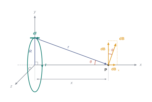
Fig. 4.9 – Magnetic field on the axis of a circular current loop.
Consider one small conducting element \(d\\vec{l}\) of the loop, as shown in Fig. 4.9. By the Biot-Savart law [Eq. 4.7(a)], the magnitude of the field \(dB\) due to this element is
\[dB = \\frac{\\mu\_0}{4\\pi},\\frac{I,|d\\vec{l}\\times\\vec{r}|}{r^3} \\tag{4.8}\]
Now, from the geometry of Fig. 4.9, \(r^2 = x^2 + R^2\). There is also a useful geometric simplification here: every element of the loop is perpendicular to the displacement vector running from that element to the axial point P. (The element \(d\\vec{l}\) in Fig. 4.9 lies in the \(y\)-\(z\) plane, while the displacement vector \(\\vec{r}\) from \(d\\vec{l}\) to the axial point P lies in the \(x\)-\(y\) plane, so the two are indeed always perpendicular.) Since \(d\\vec{l}\) and \(\\vec{r}\) are perpendicular, \(|d\\vec{l}\\times\\vec{r}| = r,dl\). This lets us simplify Eq. (4.8) to
\[dB = \\frac{\\mu\_0}{4\\pi},\\frac{I,dl}{(x^2+R^2)} \\tag{4.9}\]
The direction of \(d\\vec{B}\), as shown in Fig. 4.9, is perpendicular to the plane formed by \(d\\vec{l}\) and \(\\vec{r}\). It has one component along the axis, \(dB\_x\), and one component perpendicular to the axis, \(dB\_{\\perp}\).
Here is the key simplifying idea: when we add up the contributions from all the elements around the loop, the perpendicular components \(dB\_{\\perp}\) cancel out completely, leaving a null (zero) result. This happens because for every element \(d\\vec{l}\), there is a diametrically opposite element on the loop whose \(dB\_{\\perp}\) contribution exactly cancels it (see Fig. 4.9). As a result, only the axial component \(dB\_x\) survives after summing over the whole loop.
To find the net axial contribution, we integrate \(dB\_x = dB\\cos\\theta\) around the loop, where, from the geometry of Fig. 4.9,
\[\\cos\\theta = \\frac{R}{(x^2+R^2)^{1/2}} \\tag{4.10}\]
Combining Eqs. (4.9) and (4.10),
\[dB\_x = \\frac{\\mu\_0 I,dl}{4\\pi},\\frac{R}{(x^2+R^2)^{3/2}}\]
Summing the elements \(dl\) around the entire loop simply gives the total circumference, \(2\\pi R\). Thus, the net magnetic field at P due to the whole circular loop is
\[\\vec{B} = B\_x\\hat{i} = \\frac{\\mu\_0 I R^2}{2(x^2+R^2)^{3/2}},\\hat{i} \\tag{4.11}\]
As a useful special case, we can find the field right at the centre of the loop by setting \(x = 0\) in Eq. (4.11):
\[\\vec{B}\_0 = \\frac{\\mu\_0 I}{2R},\\hat{i} \\tag{4.12}\]
The magnetic field lines produced by a circular current loop form closed loops, as shown in Fig. 4.10. The direction of this field is given by yet another version of the right-hand thumb rule:
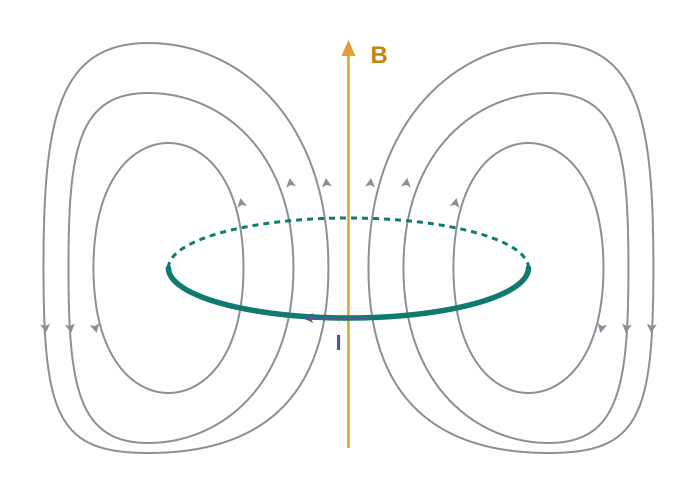
Fig. 4.10 – Magnetic field lines of a circular current loop.
Notice, from Fig. 4.10, that the upper face of the loop (the face the field lines emerge from) behaves rather like the north pole of a bar magnet, while the lower face (where the field lines return) behaves like the south pole. This resemblance between a current loop and a magnet is not a coincidence — we shall return to this important idea in Section 4.9.
A straight wire carrying a current of 12 A is bent into a semi-circular arc of radius 2.0 cm, as shown in Fig. 4.11(a). Consider the magnetic field \(\\vec{B}\) at the centre of the arc. (a) What is the contribution of the two straight segments to this field? (b) In what ways does the contribution of the semicircular part differ from — and resemble — that of a full circular loop? (c) Would the answer change if the wire were instead bent into a semicircular arc curving the opposite way, as in Fig. 4.11(b)?
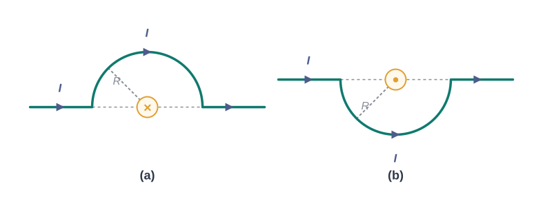
[Caption:] Fig. 4.11 – Semicircular arcs: (a) curving upward and (b) curving downward. [/Caption:]
For each element of the straight segments, \(d\\vec{l}\) and \(\\vec{r}\) point in exactly the same direction (both along the wire, towards the centre of the arc). Since the cross product of two parallel vectors is zero, \(d\\vec{l}\\times\\vec{r} = 0\) for every element of the straight parts. The straight segments therefore make no contribution at all to \(|\\vec{B}|\) at the centre.
For every element of the semicircular arc, the vector product \(d\\vec{l}\\times\\vec{r}\) points in the same direction — into the plane of the page — so all these contributions add up constructively in magnitude, just as they would for a full circular loop. The direction of \(\\vec{B}\) is given by the right-hand rule stated above, but since only half the circle’s elements are present, the magnitude works out to exactly half that of a full circular loop of the same radius. Using Eq. (4.12) with half the contribution, \(B = 1.9\\times10^{-4}\) T, directed normal to the plane of the page and going into it.
If the wire were bent the opposite way, as in Fig. 4.11(b), the magnitude of \(\\vec{B}\) would remain exactly the same as in part (b), but its direction would now be reversed, coming out of the plane of the page instead.
4.6 Ampere’s Circuital Law
The Biot-Savart law, powerful as it is, can also be expressed in an alternative and often more convenient form, known as Ampere’s circuital law. To understand this law, imagine an open surface bounded by some closed curve, or loop (Fig. 4.12). Current is allowed to pass through this surface. We think of the boundary of this surface as being built up from a large number of tiny line segments.
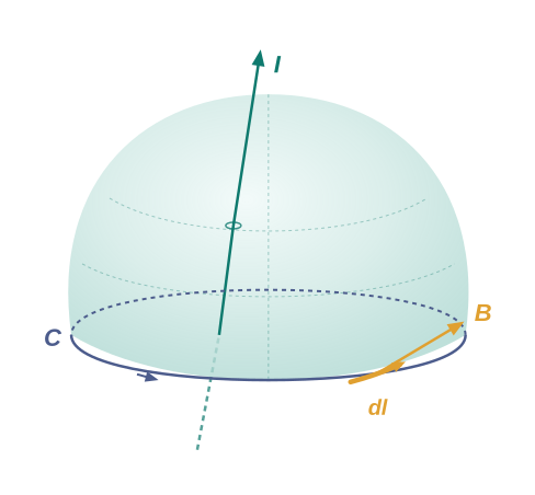
Fig. 4.12 – Ampere’s circuital law: surface bounded by loop C.
Consider one such small boundary element, of length \(dl\). At this element, take the tangential component of the magnetic field, \(B\_t\) — that is, the component of \(\\vec{B}\) pointing along the direction of the boundary itself at that point — and multiply it by the length \(dl\) of that element. (Note that \(B\_t,dl = \\vec{B}\\cdot d\\vec{l}\).) Now imagine doing this for every element around the entire boundary, and adding up all these products together.
As we take the limit where the length of each element shrinks towards zero and the number of elements grows correspondingly larger, this sum becomes a closed-loop integral. Ampere’s law states that this integral is always equal to \(\\mu\_0\) times the total current passing through the surface:
\[\\oint \\vec{B}\\cdot d\\vec{l} = \\mu\_0 I \\tag{4.13(a)}\]
where \(I\) is the total current threading through the surface, and the integral is taken all the way around the closed boundary loop \(C\) of that surface.
This relation carries with it a sign convention, fixed by the right-hand rule. If you curl the fingers of your right hand in the sense that the boundary is traversed while computing the loop integral \(\\oint\\vec{B}\\cdot d\\vec{l}\), your thumb points in the direction that is taken as the positive direction for the current \(I\).
A simplified, practical version. For many practical applications, a much simpler version of Eq. [4.13(a)] turns out to be sufficient. In these cases, it is possible to choose a loop — called an Amperian loop — such that, at every point along it, one of the following holds:
\(\\vec{B}\) is tangential to the loop and has the same non-zero, constant value \(B\) everywhere on it, or
\(\\vec{B}\) is normal (perpendicular) to the loop at every point, or
\(\\vec{B}\) is zero everywhere along that part of the loop.
If we let \(L\) denote the length of the part of the loop where \(\\vec{B}\) is tangential (case (i)), and let \(I\_e\) be the current enclosed by the loop, then Eq. (4.13) simplifies neatly to
\[BL = \\mu\_0 I\_e \\tag{4.13(b)}\]
Applying the law to a long straight wire. When a system has the right kind of symmetry — such as an infinitely long, straight current-carrying wire, shown in Fig. 4.13 — Ampere’s law provides an easy way to work out the magnetic field, in much the same way that Gauss’s law simplifies calculations of the electric field for symmetric charge distributions. This is demonstrated in Example 4.7 below.
For the infinite straight wire, we choose the Amperian loop to be a circle, since the magnetic field is tangential to the circumference of such a circle everywhere along it (by symmetry, the field cannot prefer one direction over another around the wire). Applying Eq. [4.13(b)], the left-hand side becomes \(B\\cdot 2\\pi r\). We therefore find that the magnetic field at a perpendicular distance \(r\) from the wire, outside it, is tangential to the circle and has magnitude
\[B\\times 2\\pi r = \\mu\_0 I,\\qquad B = \\frac{\\mu\_0 I}{2\\pi r} \\tag{4.14}\]
This result for the infinite wire is worth pausing over, since it reveals several interesting features:
(i) Cylindrical symmetry. The field has the same magnitude at every point on a circle of radius \(r\) centred on the wire. In other words, the field — which could, in principle, depend on all three spatial coordinates — actually depends on only one: the perpendicular distance \(r\) from the wire. This simplification, whenever it occurs, is a direct signature of an underlying symmetry in the physical situation.
(ii) Closed field lines. The field direction at every point on such a circle is tangential to it. This means the lines of constant magnetic field magnitude form closed concentric circles — exactly matching the pattern that the iron filings traced out in Oersted’s original experiment (recall Fig. 4.1(c) in Section 4.1). These closed loops of magnetic field are quite unlike electrostatic field lines, which begin at positive charges and end at negative charges, never forming closed loops on their own. The formula for the field of a straight wire, derived here from first principles, thus provides a solid theoretical explanation for exactly what Oersted observed experimentally in 1820.
(iii) The field stays finite everywhere except exactly on the wire. Even though the wire itself is (idealised as) infinitely long, the field it produces at any non-zero distance from it is not infinite. The field only threatens to blow up as we approach arbitrarily close to the wire itself. Away from the wire, the field simply falls off in direct proportion to the current and in inverse proportion to the distance.
(iv) The right-hand rule for a long wire. There is a simple rule for finding the direction of the field due to a long, straight wire: grasp the wire in your right hand, with your extended thumb pointing along the direction of current flow. Your curled fingers then indicate the direction of the magnetic field circling the wire.
How does Ampere’s law relate to the Biot-Savart law? Ampere’s circuital law is not, in any deep sense, a new or independent law separate from the Biot-Savart law — the two describe exactly the same underlying physics, and Ampere’s law can, in fact, be mathematically derived starting from the Biot-Savart law. The relationship between them closely parallels the relationship between Gauss’s law and Coulomb’s law in electrostatics: both Ampere’s law and Gauss’s law relate some physical quantity measured on the periphery, or boundary, of a region (the magnetic field or the electric field, respectively) to another physical quantity located in the interior of that region (the enclosed current, or the enclosed charge). It is also important to remember that Ampere’s circuital law, in the form given here, holds specifically for steady currents — ones that do not fluctuate with time.
Fig. 4.13 shows a long straight wire with a circular cross-section of radius \(a\), carrying a steady current \(I\) that is spread uniformly across this entire cross-section. Calculate the magnetic field in the two regions: (a) outside the wire, where \(r > a\), and (b) inside the wire, where \(r < a\).
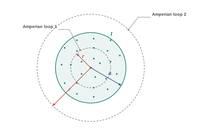
[Caption:] Fig. 4.13 – Amperian loops for a straight wire of radius a. [/Caption:]
(a) Outside the wire (\(r > a\)). Consider an Amperian loop, labelled loop 2, which is a circle of radius \(r\) concentric with the wire’s cross-section, but lying entirely outside the wire. For this loop:
\[L = 2\\pi r,\\qquad I\_e = \\text{current enclosed by the loop} = I\]
(the entire current \(I\) lies within this loop, since \(r > a\)). This gives us the familiar result for a long straight wire:
\[B(2\\pi r) = \\mu\_0 I\]
\[B = \\frac{\\mu\_0 I}{2\\pi r} \\tag{4.15(a)}\]
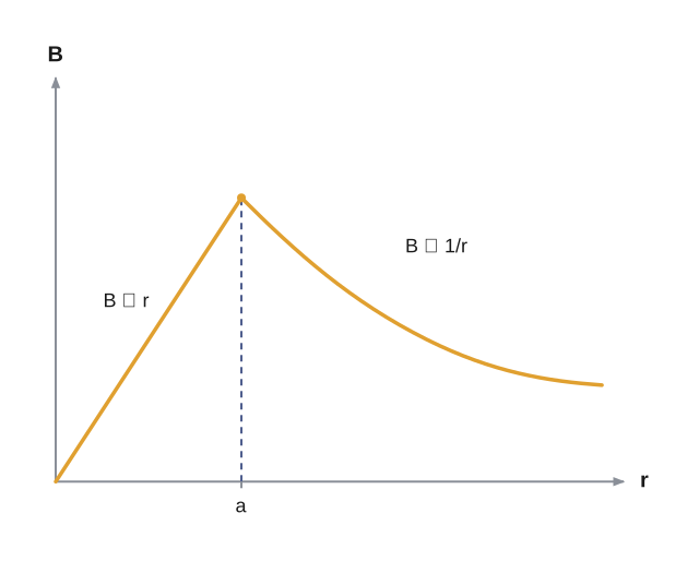
\[B \\propto \\frac{1}{r}\\qquad (r > a)\]
(b) Inside the wire (\(r < a\)). Now the current enclosed by the Amperian loop is not the full current \(I\), but only the fraction of it that flows through the smaller circle of radius \(r\). Since the current is spread uniformly across the cross-section, the enclosed current is proportional to the enclosed area:
\[I\_e = I\\left(\\frac{\\pi r^2}{\\pi a^2}\\right) = \\frac{I r^2}{a^2}\]
Applying Ampere’s law with this enclosed current,
\[B(2\\pi r) = \\mu\_0,\\frac{I r^2}{a^2}\]
\[B = \\left(\\frac{\\mu\_0 I}{2\\pi a^2}\\right) r \\tag{4.15(b)}\]
\[B\\propto r\\qquad (r < a)\]
Fig. 4.14 shows a plot of the magnitude of \(B\) against the distance \(r\) from the centre of the wire — rising linearly inside the wire, reaching a maximum right at the surface (\(r = a\)), and then falling off as \(1/r\) outside the wire. The direction of the field at any point is tangential to the appropriate circular loop (1 or 2), and is given by the right-hand rule described earlier.
[Caption:] Fig. 4.14 – Variation of magnetic field with distance from the wire’s centre. [/Caption:]
This example possesses exactly the kind of symmetry needed for Ampere’s law to be applied easily and directly.
It should be emphasised that although Ampere’s circuital law holds true for any closed loop whatsoever, it does not always make it easy to calculate the magnetic field — that only happens when the chosen loop matches the symmetry of the current distribution well. For example, in the case of the circular current loop discussed in Section 4.5, Ampere’s law cannot conveniently be used to derive the simple expression \(B = \\mu\_0 I/2R\) [Eq. (4.12)] for the field at the centre of the loop, because no simple Amperian loop matches that geometry’s symmetry. Nonetheless, there exists a wide range of situations with high symmetry where the law can be applied very conveniently — and we shall use exactly this approach in the next section to work out the magnetic field of a solenoid.
4.7 The Solenoid
We now turn to a very useful and widely used magnetic device: the solenoid. Here, we restrict our discussion to a long solenoid, meaning one whose length is large compared to its radius. A solenoid consists of a long wire wound in the shape of a helix, with neighbouring turns spaced closely together. Because the turns are so closely spaced, each individual turn can be treated, to a good approximation, as a simple circular loop of current. The overall magnetic field produced by the solenoid is then just the vector sum of the fields due to every one of these turns. In practice, the wire used for winding is enamelled (coated with a thin insulating layer), so that neighbouring turns do not electrically short-circuit each other.
Fig. 4.15 shows the magnetic field lines for a finite (not infinitely long) solenoid. A section of this solenoid is shown enlarged, for clarity, in Fig. 4.15(a), while Fig. 4.15(b) shows the field of the entire finite solenoid.
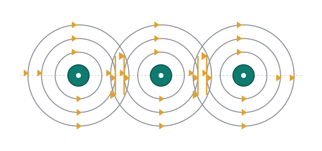
Fig. 4.15(a) – Cancellation of magnetic field between adjacent solenoid turns.
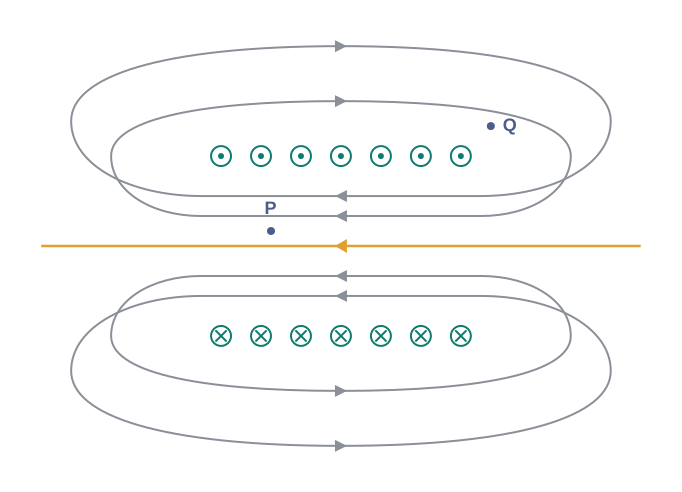
Fig. 4.15(b) – Magnetic field pattern of a finite solenoid.
Looking at Fig. 4.15(a), it becomes clear from the individual circular field loops around each turn that the field between two neighbouring turns essentially cancels out. Meanwhile, Fig. 4.15(b) shows that at the interior mid-point, labelled P, the field is uniform, strong, and directed along the axis of the solenoid. By contrast, at the exterior mid-point, labelled Q, the field is weak — and, notably, it still points along the solenoid’s axis, with no component perpendicular or normal to that axis.
As the solenoid is made longer and longer, this pattern becomes even cleaner, and the solenoid begins to resemble a long cylindrical metal sheet carrying current around its surface, as idealised in Fig. 4.16. In this ideal, very-long-solenoid limit, we make two simplifying assumptions: the field outside the solenoid is taken to be exactly zero, and the field everywhere inside becomes uniform and parallel to the axis.
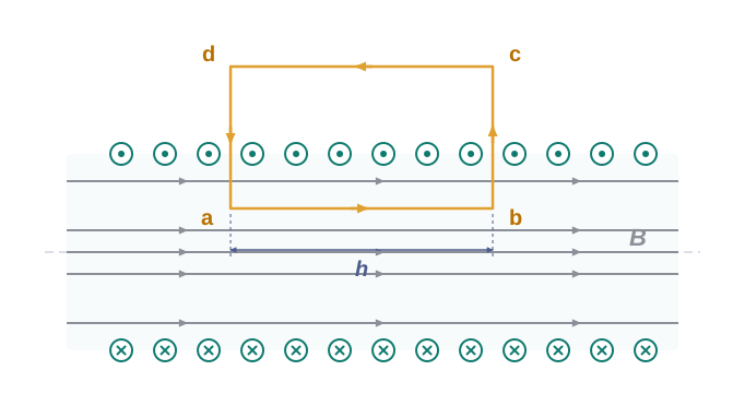
Fig. 4.16 – Amperian loop for a long ideal solenoid.
Applying Ampere’s law to the solenoid. To calculate the interior field, consider a rectangular Amperian loop \(abcd\), as drawn in Fig. 4.16, with side \(ab\) lying along the solenoid’s axis inside it, and side \(cd\) lying entirely outside the solenoid. Along \(cd\), the field is zero, as argued above. Along the two transverse sides, \(bc\) and \(ad\), the field component along the direction of travel is zero (since the field inside is axial, and these sides run perpendicular to the axis), so these two sides make no contribution to the loop integral either. That leaves only the side \(ab\), along which we call the field \(B\). So the only length of the Amperian loop that matters is \(L = h\), the length of side \(ab\).
Let \(n\) be the number of turns per unit length of the solenoid. Then the total number of turns enclosed within a length \(h\) of the loop is \(nh\). Since each of these turns carries current \(I\), the total enclosed current is \(I\_e = I(nh)\). Applying Ampere’s circuital law [Eq. 4.13(b)]:
\[BL = \\mu\_0 I\_e,\\qquad Bh = \\mu\_0 I(nh)\]
\[B = \\mu\_0 n I \\tag{4.16}\]
The direction of this field is given by the same right-hand rule used for a single circular loop (Section 4.5): curl your fingers along the direction the current flows in the turns, and your thumb points along the direction of the axial field.
The solenoid is, in fact, one of the most common and practical ways to obtain a uniform magnetic field in the laboratory or in engineering applications. In the next chapter, we shall see that an even larger field can be obtained from the same solenoid, and the same current, simply by inserting a soft iron core into its centre.
4.8 Force between Two Parallel Currents, the Ampere
By now we have learnt two important facts. First, a current-carrying conductor produces a magnetic field in the space around it, in accordance with the Biot-Savart law. Second, an external magnetic field exerts a force on a current-carrying conductor placed in it, as a direct consequence of the Lorentz force. Putting these two facts together leads to a natural expectation: if we place two current-carrying conductors near each other, then each one sits in the magnetic field produced by the other, so each should exert a magnetic force on the other.
This is exactly what happens, and it is a phenomenon that Ampere studied in great detail. In the period 1820–25, Ampere carefully investigated the nature of this magnetic force between conductors — how it depends on the magnitude of the currents, on the shape and size of the conductors, and on the distances separating them. In this section, we take the simplest possible case, two long parallel current-carrying conductors, which will help us appreciate the essence of Ampere’s painstaking experimental work.
Setting up the problem. Fig. 4.17 shows two long parallel conductors, labelled \(a\) and \(b\), separated by a distance \(d\), carrying currents \(I\_a\) and \(I\_b\) respectively, both flowing in the same direction (parallel currents).
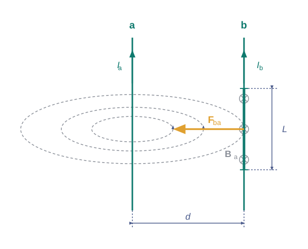
Fig. 4.17 – Magnetic force between two parallel current-carrying conductors.
The conductor \(a\) produces a magnetic field at every point along the conductor \(b\). Because \(a\) is a long straight wire, this field has the same magnitude \(B\_a\) everywhere along \(b\). Using the right-hand rule, the direction of this field (when the conductors are laid out horizontally) points downwards along \(b\). From Eq. [4.15(a)] — or equivalently from Ampere’s circuital law — its magnitude is
\[B\_a = \\frac{\\mu\_0 I\_a}{2\\pi d}\]
Here \(\\mu\_0\) is the permeability of free space, \(I\_a\) is the current in conductor \(a\), and \(d\) is the perpendicular distance between the two conductors.
Force on conductor b. The conductor \(b\), carrying current \(I\_b\), now sits in this field \(B\_a\) and therefore experiences a sideways force. Working out the direction (which you should verify for yourself using the right-hand rule) shows that this force points towards conductor \(a\). We label this force \(\\vec{F}\_{ba}\) — the force on a segment of length \(L\) of conductor \(b\) due to conductor \(a\). Its magnitude follows from Eq. (4.4), \(F = I l B\), with the current and field perpendicular:
\[F\_{ba} = I\_b L B\_a = \\frac{\\mu\_0 I\_a I\_b}{2\\pi d},L \\tag{4.17}\]
Force on conductor a, and Newton’s third law. By exactly the same reasoning, we could instead work out the force on conductor \(a\) due to the field produced by conductor \(b\). Following identical steps, we would find a force \(\\vec{F}*{ab}\) on a segment of length \(L\) of conductor \(a\), equal in magnitude to \(F*{ba}\), but this time directed towards conductor \(b\). Thus
\[\\vec{F}*{ba} = -\\vec{F}*{ab} \\tag{4.18}\]
Notice that this result is fully consistent with Newton’s third law: the two conductors push on each other with equal and opposite forces. In other words, at least for the case of parallel conductors carrying steady currents, we have shown that the Biot-Savart law and the Lorentz force together yield results in agreement with Newton’s third law.
Attraction and repulsion. In the case just analysed, both currents flowed in the same direction, and we found that the forces pull the two conductors towards each other — that is, parallel currents attract. A similar analysis (which you can carry out yourself) shows that if the two currents flow in opposite directions, the forces push the conductors apart. This gives us a compact and important rule:
It is worth pausing to notice how this rule differs from the corresponding rule in electrostatics. There, like (same-sign) charges repel each other. Here, like (parallel) currents attract each other — the opposite behaviour. This contrast is a striking reminder that magnetic interactions between currents follow their own distinct rules, and cannot simply be guessed by analogy with static charges.
Force per unit length. Let \(f\_{ba}\) denote the magnitude of the force \(\\vec{F}\_{ba}\) per unit length of the conductor. Dividing Eq. (4.17) by the length \(L\),
\[f\_{ba} = \\frac{\\mu\_0 I\_a I\_b}{2\\pi d} \\tag{4.19}\]
This deceptively simple expression is of fundamental importance, because it is used to define the ampere (A) — one of the seven SI base units.
Defining the ampere. By choosing specific standard values in Eq. (4.19), we arrive at the formal definition of the ampere.
This definition of the ampere was adopted in 1946. It is a theoretical definition — an idealisation involving infinitely long, infinitely thin wires. In actual practice, one must eliminate the effect of the Earth’s magnetic field and replace the very long straight wires by multiturn coils of suitable geometry. An instrument called the current balance is used to measure this small mechanical force in the laboratory.
Defining the coulomb. Once the ampere is defined, the SI unit of electric charge — the coulomb — can be defined in terms of it.
4.9 Torque on Current Loop, Magnetic Dipole
4.9.1 Torque on a rectangular current loop in a uniform magnetic field
We now show an important result: a rectangular loop carrying a steady current \(I\), when placed in a uniform magnetic field, experiences a torque — a turning effect — even though it experiences no net translational force. (Recall that a torque is the rotational equivalent of a force: it is what causes an object to rotate rather than simply move from place to place.) This behaviour is closely analogous to that of an electric dipole placed in a uniform electric field, which you studied in Section 1.11.
Case 1: field in the plane of the loop. Let us begin with the simple case where the uniform magnetic field \(\\vec{B}\) lies in the plane of the loop, as illustrated in Fig. 4.18(a).
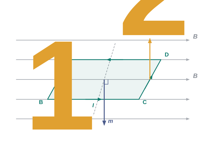
Fig. 4.18(a) – Rectangular loop in a magnetic field lying in its plane.
In this arrangement, the field exerts no force on the two arms AD and BC of the loop. However, the field is perpendicular to arm AB, and exerts a force \(\\vec{F}\_1\) on it, directed into the plane of the loop. Using Eq. (4.4), its magnitude is
\[F\_1 = I b B\]
where \(b\) is the length of arm AB. Similarly, the field exerts a force \(\\vec{F}\_2\) on the opposite arm CD, directed out of the plane of the paper, with the same magnitude:
\[F\_2 = I b B = F\_1\]
Since \(\\vec{F}\_1\) and \(\\vec{F}\_2\) are equal in magnitude but opposite in direction, the net force on the loop is zero. But these two forces do not act along the same line — they form what is called a couple, and a couple produces a torque. Fig. 4.18(b) shows a view of the loop looking from the AD end, and makes clear that this torque tends to rotate the loop anticlockwise.
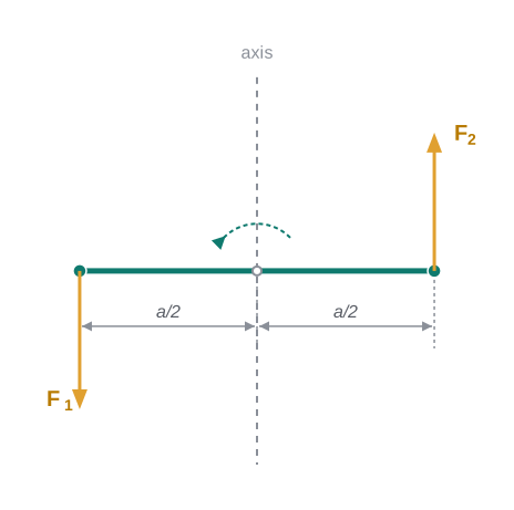
Fig. 4.18(b) – End-on view showing the torque-producing couple.
The magnitude of this torque is found by adding the moments of the two forces about the central axis. Each force acts at a perpendicular distance \(a/2\) from the axis (where \(a\) is the length of the other pair of arms):
\[\\tau = F\_1\\frac{a}{2} + F\_2\\frac{a}{2} = IbB\\frac{a}{2} + IbB\\frac{a}{2} = I(ab)B = IAB \\tag{4.20}\]
where \(A = ab\) is the area of the rectangular loop.
Case 2: field at an angle to the loop. Now consider the more general case, where the plane of the loop is not aligned with the magnetic field, but the normal to the loop makes an angle \(\\theta\) with the field. (The previous case corresponds to \(\\theta = \\pi/2\), since then the loop’s plane contains the field.) This general situation is shown in Fig. 4.19.
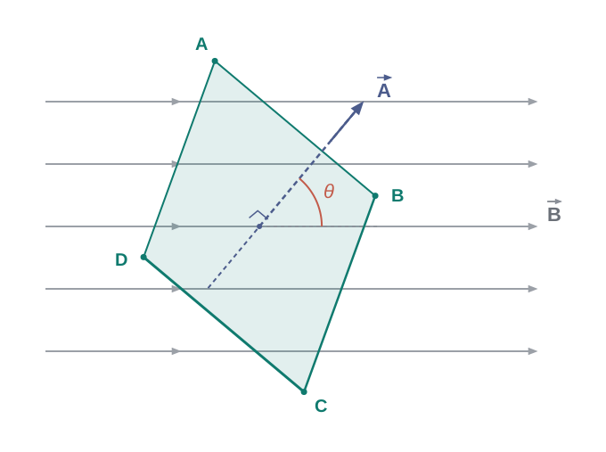
Fig. 4.19(a) – Area vector of loop making an angle θ with the field.
In this configuration, the forces on arms BC and DA are equal, opposite, and act along the same line (the axis of the coil, connecting the midpoints of BC and DA). Being collinear, they cancel completely, producing neither net force nor torque. The forces on arms AB and CD, however, are again \(\\vec{F}\_1\) and \(\\vec{F}\_2\), equal and opposite in magnitude,
\[F\_1 = F\_2 = I b B\]
but this time they are not collinear, so once again they form a couple. The resulting torque, however, is now smaller than in the previous case. This is because the perpendicular distance between the lines of action of the two forces has decreased as the loop rotated away from the field-in-plane orientation. Fig. 4.19(b) shows this couple viewed from the AD end.
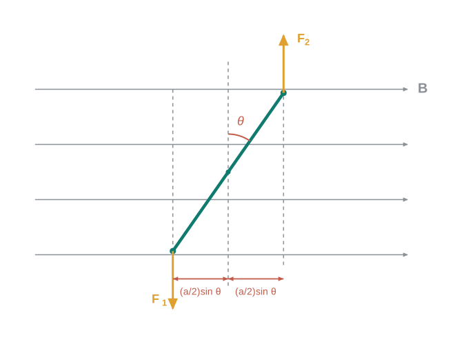
Fig. 4.19(b) – Top view showing the reduced moment arm.
The magnitude of the torque on the loop in this general case is
\[\\tau = F\_1\\frac{a}{2}\\sin\\theta + F\_2\\frac{a}{2}\\sin\\theta = I,ab,B\\sin\\theta = IAB\\sin\\theta \\tag{4.21}\]
As \(\\theta\\to 0\) — that is, as the normal to the loop lines up with the field — the perpendicular distance between the two forces of the couple also approaches zero. This makes the two forces collinear, so both the net force and the net torque become zero.
Introducing the magnetic moment. Both Eqs. (4.20) and (4.21) can be written far more compactly using a vector cross product, by introducing a new quantity called the magnetic moment of the current loop. We define it as
\[\\vec{m} = I\\vec{A} \\tag{4.22}\]
where the direction of the area vector \(\\vec{A}\) is fixed by the right-hand thumb rule (in Fig. 4.18, it is directed into the plane of the paper). With this definition, since the angle between \(\\vec{m}\) and \(\\vec{B}\) is \(\\theta\), both Eqs. (4.20) and (4.21) combine into a single elegant expression:
\[\\vec{\\tau} = \\vec{m}\\times\\vec{B} \\tag{4.23}\]
This is directly analogous to the electrostatic case you met in Chapter 1, where an electric dipole of dipole moment \(\\vec{p}\_e\) in an electric field \(\\vec{E}\) experiences a torque \(\\vec{\\tau} = \\vec{p}\_e\\times\\vec{E}\). From Eq. (4.22), we can read off the dimensions of the magnetic moment as \(\[A]\[L^2]\), giving the unit A m\(^2\), as stated.
Equilibrium of the loop. From Eq. (4.23), the torque \(\\vec{\\tau}\) vanishes whenever \(\\vec{m}\) is either parallel or antiparallel to the magnetic field \(\\vec{B}\). Both of these represent states of equilibrium, since there is no torque to rotate the coil (this reasoning applies to any object carrying a magnetic moment \(\\vec{m}\), not just current loops).
However, the two equilibria differ in character. When \(\\vec{m}\) and \(\\vec{B}\) are parallel, the equilibrium is stable: any small rotation of the coil produces a restoring torque that brings it back to its original position. When they are antiparallel, the equilibrium is unstable: any small rotation produces a torque that grows larger and pushes the coil further away from that position. This same tendency — for a magnetic moment to align itself with an external field — is exactly why a small magnet, or any magnetic dipole, spontaneously turns to point along an external magnetic field.
Loops with many turns. If the loop has \(N\) closely wound turns instead of a single turn, the expression for torque, Eq. (4.23), still holds, but with the magnetic moment now given by
\[\\vec{m} = NI\\vec{A} \\tag{4.24}\]
4.9.2 Circular current loop as a magnetic dipole
In this section, we take up the most elementary magnetic element of all: the current loop itself. We shall show that at large distances, the magnetic field produced by a circular current loop is very similar in form to the electric field of an electric dipole — which is why a current loop is regarded as a magnetic dipole.
Recall from Section 4.5 that the magnetic field on the axis of a circular loop of radius \(R\), carrying a steady current \(I\), has magnitude [Eq. (4.11)]
\[B = \\frac{\\mu\_0 I R^2}{2(x^2+R^2)^{3/2}}\]
directed along the axis (with direction given by the right-hand thumb rule, Fig. 4.10), where \(x\) is the distance along the axis from the centre of the loop.
Now consider points very far from the loop, where \(x \\gg R\). In this regime, the \(R^2\) term in the denominator becomes negligible compared with \(x^2\), and can be dropped. This simplifies the field to
\[B = \\frac{\\mu\_0 I R^2}{2x^3}\]
Recalling that the area of the loop is \(A = \\pi R^2\), so that \(R^2 = A/\\pi\), we can rewrite this as
\[B = \\frac{\\mu\_0 I A}{2\\pi x^3}\]
As before, we define the magnetic moment of the loop to have magnitude \(m = IA\), so \(\\vec{m} = I\\vec{A}\). In terms of the magnetic moment,
\[B \\simeq \\frac{\\mu\_0 m}{2\\pi x^3} = \\frac{\\mu\_0}{4\\pi},\\frac{2m}{x^3} \\tag{4.25(a)}\]
The expression in Eq. [4.25(a)] is strikingly similar to the one you obtained in Chapter 1 for the electric field of an electric dipole along its axis. The correspondence becomes explicit if we make the substitution \(\\mu\_0 \\to 1/\\varepsilon\_0\), along with \(\\vec{m}\\to\\vec{p}\_e\) (magnetic moment replaced by electric dipole moment) and \(\\vec{B}\\to\\vec{E}\) (magnetic field replaced by electric field). Then Eq. [4.25(a)] becomes
\[\\vec{E} = \\frac{2\\vec{p}\_e}{4\\pi\\varepsilon\_0 x^3}\]
which is precisely the field of an electric dipole at a point on its axis, as derived in Chapter 1, Section 1.9 [Eq. (1.20)].
This analogy can be pushed even further. In Chapter 1, you found that the electric field on the perpendicular bisector of an electric dipole is given by [Eq. (1.21)]
\[E \\simeq \\frac{p\_e}{4\\pi\\varepsilon\_0 x^3}\]
where \(x\) is the distance from the dipole. If we again replace \(\\vec{p}\\to\\vec{m}\) and \(\\mu\_0\\to 1/\\varepsilon\_0\) in this expression, we obtain the result for \(\\vec{B}\) at a point in the plane of the loop, at a distance \(x\) from the centre (for \(x \\gg R\)):
\[\\vec{B} = \\frac{\\mu\_0}{4\\pi},\\frac{\\vec{m}}{x^3},;\\qquad x \\gg R \\tag{4.25(b)}\]
The results given by Eqs. [4.25(a)] and [4.25(b)] become exact in the limit of a point magnetic dipole.
The results obtained above turn out to apply not just to a circular loop, but to any planar current loop whatsoever: a planar current loop is equivalent to a magnetic dipole of dipole moment \(\\vec{m} = I\\vec{A}\), which is the magnetic analogue of the electric dipole moment \(\\vec{p}\).
There is, however, one deep and fundamental difference between the two kinds of dipole. An electric dipole is built up from two more elementary units — the positive and negative charges (the electric “monopoles”). In magnetism, by contrast, the magnetic dipole (or current loop) is itself the most elementary magnetic element. The magnetic equivalent of an isolated electric charge — an isolated magnetic pole, or magnetic monopole — has never been observed to exist.
We have now shown two things about a current loop: (i) it produces a magnetic field and behaves like a magnetic dipole at large distances (see Fig. 4.10), and (ii) it experiences a torque when placed in an external field, just like a magnetic needle would. Together, these facts led Ampere to make a bold suggestion: that all magnetism might ultimately be due to circulating electric currents. This idea turns out to be partly true, and no magnetic monopoles have ever been found. However, the story is not quite complete: elementary particles such as the electron and the proton also carry an intrinsic magnetic moment — a magnetic moment built into the particle itself — which cannot be accounted for by any picture of circulating currents.
4.10 The Moving Coil Galvanometer
Currents and voltages in electric circuits were discussed at length in Chapter 3. But a practical question was left unanswered there: how do we actually measure them? How can we confidently claim that the current in a circuit is 1.5 A, or that the voltage drop across a resistor is 1.2 V? Fig. 4.20 shows a very useful instrument built for exactly this purpose — the moving coil galvanometer (MCG) — whose working principle can be understood directly from the discussion of torque on a current loop in Section 4.9.
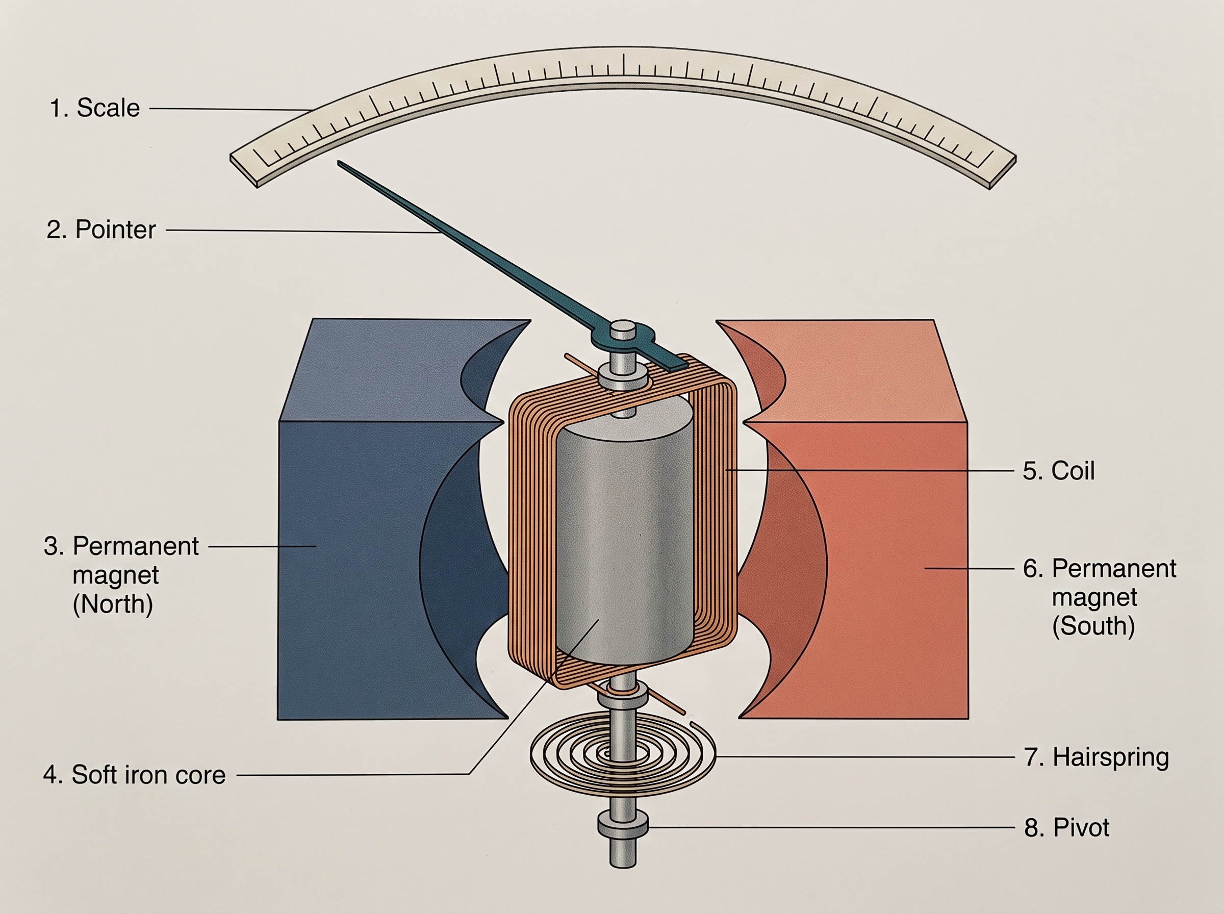
Fig. 4.20 – The moving coil galvanometer.
Construction and working. The galvanometer consists of a coil with many turns, mounted so that it is free to rotate about a fixed axis, sitting in a uniform radial magnetic field (Fig. 4.20). A cylindrical soft iron core is placed inside the coil; this core serves two purposes at once — it makes the magnetic field radial in shape, and it also increases the strength of the field. When a current flows through the coil, the magnetic field exerts a torque on it, which (from Eq. 4.20) has magnitude
\[\\tau = NIAB\]
where the symbols have their usual meanings (\(N\) = number of turns, \(I\) = current, \(A\) = area of the coil, \(B\) = magnetic field). Notice that here we have taken \(\\sin\\theta = 1\) in the torque expression — this is possible precisely because the field is designed to be radial. In a radial field, the plane of the coil always contains the field direction no matter how far the coil has rotated, so the angle between the field and the coil’s normal is always 90°, keeping \(\\sin\\theta = 1\) at all deflections. This is a clever design feature: it makes the torque independent of the coil’s angular position, which in turn makes the instrument’s scale evenly spaced (linear).
Reaching equilibrium. The magnetic torque \(NIAB\) tends to rotate the coil. A spring \(S\_p\) opposes this rotation, providing a counter (restoring) torque \(k\\phi\) that balances the magnetic torque. The coil rotates until these two torques are equal, settling at a steady angular deflection \(\\phi\). At this equilibrium:
\[k\\phi = NIAB\]
where \(k\) is the torsional constant of the spring — the restoring torque produced per unit angle of twist. The deflection \(\\phi\) is read off on the scale by a pointer attached to the spring. Rearranging,
\[\\phi = \\left(\\frac{NAB}{k}\\right)I \\tag{4.26}\]
The quantity in brackets, \(NAB/k\), is a constant for any given galvanometer. This means the deflection \(\\phi\) is directly proportional to the current \(I\) — which is exactly what makes the galvanometer useful as a measuring instrument.
Using the galvanometer as a detector. The galvanometer can be used in several ways. In its simplest role, it acts as a detector — a device to check whether any current is flowing in a circuit at all. You have already come across this usage in the Wheatstone bridge arrangement in Chapter 3. In this role, the pointer’s neutral (zero-current) position is set in the middle of the scale rather than at the left end shown in Fig. 4.20, so that depending on the direction of current flow, the pointer can deflect either to the right or to the left.
Why a galvanometer cannot directly serve as an ammeter. An ammeter is an instrument for measuring the actual value of the current in a circuit. A galvanometer, as it stands, cannot serve this purpose directly, for two reasons. First, it is a very sensitive device — it gives a full-scale deflection for currents as small as the order of microamperes (\(\\mu\)A), so ordinary circuit currents would swing the pointer far off the scale. Second, to measure a current, the instrument must be connected in series with the circuit; but since a galvanometer has a relatively large resistance, inserting it in series would significantly change the very current it is meant to measure.
Converting a galvanometer into an ammeter. To overcome these difficulties, a small resistance \(r\_s\), called a shunt resistance, is connected in parallel with the galvanometer coil. Most of the current then passes through the low-resistance shunt, and only a small, known fraction passes through the galvanometer itself. The combined resistance of this parallel arrangement is
\[\\frac{R\_G, r\_s}{R\_G + r\_s} \\simeq r\_s \\qquad \\text{if}\\quad R\_G \\gg r\_s\]
Fig. 4.21 – Conversion of a galvanometer into an ammeter.
If \(r\_s\) is very small in relation to the resistance of the rest of the circuit \(R\_c\), then the effect of inserting the measuring instrument on the circuit’s current is also small and negligible. This arrangement is shown schematically in Fig. 4.21. The scale of such an ammeter is calibrated and graduated so that the current value can be read off directly and with ease.
A convenient way for a manufacturer to increase this sensitivity is simply to increase the number of turns \(N\) in the coil. In practice, one chooses a galvanometer whose sensitivity suits the particular experiment at hand.
Converting a galvanometer into a voltmeter. The galvanometer can also be adapted to serve as a voltmeter, measuring the voltage across a chosen section of a circuit. For this, it must be connected in parallel with that section. Crucially, a voltmeter must draw only a very small current, otherwise the act of measuring would itself disturb the original circuit significantly. (We usually like to keep this disturbance below one per cent.) To ensure this, a large resistance \(R\) is connected in series with the galvanometer. This arrangement is shown in Fig. 4.22. Note that the total resistance of the voltmeter is now
\[R\_G + R \\simeq R \\qquad (\\text{large})\]
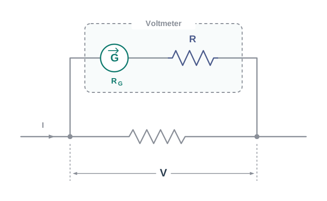
Fig. 4.22 – Conversion of a galvanometer into a voltmeter.
The scale of this voltmeter is calibrated to read off voltage directly. We define the voltage sensitivity as the deflection per unit voltage. From Eq. (4.26),
\[\\frac{\\phi}{V} = \\left(\\frac{NAB}{k}\\right)\\frac{I}{V} = \\left(\\frac{NAB}{k}\\right)\\frac{1}{R} \\tag{4.28}\]
A subtle but important point. It might seem that increasing the current sensitivity should automatically increase the voltage sensitivity too — but this is not necessarily so. To see why, take Eq. (4.27) for the current sensitivity. Suppose we double the number of turns, \(N\\to 2N\). Then
\[\\frac{\\phi}{I}\\to 2\\frac{\\phi}{I}\]
so the current sensitivity indeed doubles. However, doubling the number of turns also roughly doubles the resistance of the galvanometer coil, since resistance is proportional to the length of wire used, so \(R\\to 2R\). Looking now at Eq. (4.28) for the voltage sensitivity, with both \(N\\to 2N\) and \(R\\to 2R\):
\[\\frac{\\phi}{V}\\to\\frac{\\phi}{V}\]
the voltage sensitivity remains unchanged. So, in general, the modification needed to convert a galvanometer into a good ammeter is different from what is needed to convert it into a good voltmeter — a genuinely useful insight for anyone designing or choosing measuring instruments.
In the circuit of Fig. 4.23, the current is to be measured. What is the value of the current if the ammeter shown is (a) a galvanometer with resistance \(R\_G = 60.00\\ \\Omega\); (b) the galvanometer of (a) converted into an ammeter by a shunt resistance \(r\_s = 0.02\\ \\Omega\); (c) an ideal ammeter with zero resistance?
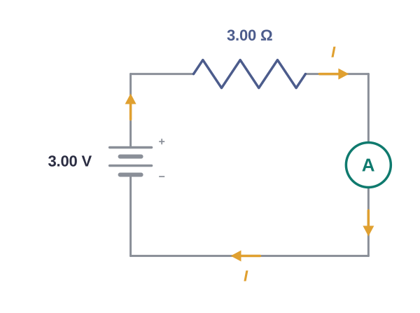
[Caption:] Fig. 4.23 – Circuit for measuring current. [/Caption:]
(a) With the galvanometer in the circuit, the total resistance is \(R\_G + 3 = 63\\ \\Omega\). Hence
\[I = 3/63 = 0.048\\ \\text{A}\]
(b) The resistance of the galvanometer converted into an ammeter (galvanometer in parallel with the shunt) is
\[\\frac{R\_G, r\_s}{R\_G + r\_s} = \\frac{60\\ \\Omega\\times0.02\\ \\Omega}{(60+0.02),\\Omega}\\simeq 0.02\\ \\Omega\]
The total resistance in the circuit is then \(0.02\\ \\Omega + 3\\ \\Omega = 3.02\\ \\Omega\). Hence
\[I = 3/3.02 = 0.99\\ \\text{A}\]
(c) For an ideal ammeter with zero resistance, the total resistance is just the \(3\\ \\Omega\) resistor, so
\[I = 3/3 = 1.00\\ \\text{A}\]
Notice how dramatically the answers differ: the bare galvanometer (a) badly disturbs the circuit and reads only 0.048 A, whereas the properly shunted ammeter (b) reads 0.99 A — very close to the ideal 1.00 A of case (c). This is a concrete demonstration of why the shunt resistance is essential for accurate current measurement.
4.11 Summary
- The total force on a charge \(q\) moving with velocity \(\\vec{v}\) in the presence of both a magnetic field \(\\vec{B}\) and an electric field \(\\vec{E}\) is called the Lorentz force. It is given by \[\\vec{F} = q(\\vec{v}\\times\\vec{B} + \\vec{E})\] The magnetic part of this force, \(q(\\vec{v}\\times\\vec{B})\), is always perpendicular (“normal”) to \(\\vec{v}\), so the work done by it is zero — it changes the direction of motion but never the speed.
- A straight conductor of length \(l\) carrying a steady current \(I\), placed in a uniform external magnetic field \(\\vec{B}\), experiences a force \[\\vec{F} = I\\vec{l}\\times\\vec{B}\] where \(|\\vec{l}| = l\), and the direction of \(\\vec{l}\) is the direction in which the current flows.
- In a uniform magnetic field \(\\vec{B}\), a charge \(q\) moving perpendicular to the field travels in a circular orbit lying in a plane normal to \(\\vec{B}\). The frequency of this uniform circular motion, called the cyclotron frequency, is \[\\nu\_c = \\frac{qB}{2\\pi m}\] Remarkably, this frequency does not depend on the particle’s speed or on the radius of its orbit. This fact is exploited in the cyclotron, a machine used to accelerate charged particles to high energies.
- The Biot-Savart law states that the magnetic field \(d\\vec{B}\) produced by a current element \(d\\vec{l}\), carrying a steady current \(I\), at a point P situated a distance \(r\) from the element, is \[d\\vec{B} = \\frac{\\mu\_0}{4\\pi},I,\\frac{d\\vec{l}\\times\\vec{r}}{r^3}\] To find the total field at P, this vector expression must be integrated over the entire length of the conductor.
- The magnitude of the magnetic field due to a circular coil of radius \(R\) carrying current \(I\), at an axial distance \(x\) from the centre, is \[B = \\frac{\\mu\_0 I R^2}{2(x^2+R^2)^{3/2}}\] At the centre of the coil (\(x = 0\)), this reduces to \[B = \\frac{\\mu\_0 I}{2R}\]
- Ampere’s Circuital Law: For an open surface S bounded by a closed loop C, the law states that \[\\oint\_C \\vec{B}\\cdot d\\vec{l} = \\mu\_0 I\] where \(I\) is the total current passing through the surface S, and its sign is fixed by the right-hand rule. A simplified form is often useful: if \(\\vec{B}\) is directed along the tangent at every point of a closed curve of length \(L\), and is constant in magnitude along it, then \[BL = \\mu\_0 I\_e\] where \(I\_e\) is the net current enclosed by the closed curve.
- The magnitude of the magnetic field at a perpendicular distance \(R\) from a long, straight wire carrying a current \(I\) is \[B = \\frac{\\mu\_0 I}{2\\pi R}\] The field lines form circles concentric with the wire.
- The magnitude of the field \(B\) inside a long solenoid carrying a current \(I\) is \[B = \\mu\_0 n I\] where \(n\) is the number of turns per unit length.
- Parallel currents attract each other, and anti-parallel currents repel each other. (This is the opposite of the electrostatic rule for charges, where like charges repel.)
- A planar loop carrying a current \(I\), with \(N\) closely wound turns and an area \(A\), possesses a magnetic moment \[\\vec{m} = NI\\vec{A}\] The direction of \(\\vec{m}\) is given by the right-hand thumb rule: curl the palm of your right hand along the loop with the fingers pointing in the direction of the current, and the outstretched thumb gives the direction of \(\\vec{m}\) (and of \(\\vec{A}\)). When this loop is placed in a uniform magnetic field \(\\vec{B}\), the net force on it is \[\\vec{F} = 0\] and the torque on it is \[\\vec{\\tau} = \\vec{m}\\times\\vec{B}\] In a moving coil galvanometer, this torque is balanced by a counter-torque from a spring, giving \[k\\phi = NIAB\] where \(\\phi\) is the equilibrium deflection and \(k\) is the torsion constant of the spring.
- A moving coil galvanometer can be converted into an ammeter by connecting a shunt resistance \(r\_s\) of small value in parallel with it. It can be converted into a voltmeter by connecting a resistance of large value in series with it.
Table of Key Physical Quantities
| Physical Quantity | Symbol | Nature | Dimensions | SI Unit | Remarks |
|---|---|---|---|---|---|
| Permeability of free space | \(\\mu\_0\) | Scalar | \(\[\\text{MLT}^{-2}\\text{A}^{-2}]\) | T m A\(^{-1}\) | \(4\\pi\\times10^{-7}\) T m A\(^{-1}\) |
| Magnetic Field | \(\\vec{B}\) | Vector | \(\[\\text{M T}^{-2}\\text{A}^{-1}]\) | T (tesla) | |
| Magnetic Moment | \(\\vec{m}\) | Vector | \(\[\\text{L}^2\\text{A}]\) | A m\(^2\) or J/T | |
| Torsion Constant | \(k\) | Scalar | \(\[\\text{M L}^2\\text{T}^{-2}]\) | N m rad\(^{-1}\) | Appears in MCG |
4.12 Points to Ponder
- Electrostatic field lines always begin at a positive charge and end at a negative charge (or fade away at infinity). Magnetic field lines behave very differently: they always form closed loops, with no beginning and no end. This reflects a deep fact — there are no isolated magnetic “charges” (monopoles) for field lines to start from or terminate on.
- Everything discussed in this chapter applies specifically to steady currents — currents that do not change with time. A word of caution about Newton’s third law: when currents do vary with time, Newton’s third law holds true only if we also account for the momentum carried by the electromagnetic field itself, not just the momentum of the charges and conductors.
- Recall the expression for the Lorentz force, \[\\vec{F} = q(\\vec{v}\\times\\vec{B} + \\vec{E})\] This velocity-dependent force has occupied the attention of some of the greatest thinkers in physics, because it hides a subtle puzzle. Suppose you switch to a reference frame moving instantaneously with velocity \(\\vec{v}\) — the same velocity as the charge. In that frame, the charge is momentarily at rest, so the magnetic part of the force (\(q\\vec{v}\\times\\vec{B}\)) vanishes entirely. Yet the charge must still behave the same way physically. The motion is then explained by saying that, in this new frame, an appropriate electric field appears that accounts for the effect. We shall not go into the details of this mechanism here. But the resolution of this apparent paradox carries a profound message: electricity and magnetism are not separate phenomena but two aspects of a single, linked phenomenon — electromagnetism — and the Lorentz force does not single out any universally preferred frame of reference in nature.
- Ampere’s Circuital Law is not an independent law, separate from the Biot-Savart law. It can, in fact, be derived from the Biot-Savart law. The relationship between the two is closely parallel to the relationship between Gauss’s law and Coulomb’s law in electrostatics — in each pair, one law relates a field on a boundary to the source enclosed within, while the other gives the field directly from each element of the source.
4.13 NCERT Questions
- A circular coil of wire consisting of 100 turns, each of radius 8.0 cm, carries a current of 0.40 A. What is the magnitude of the magnetic field \(\\vec{B}\) at the centre of the coil?
- A long straight wire carries a current of 35 A. What is the magnitude of the field \(\\vec{B}\) at a point 20 cm from the wire?
- A long straight wire in the horizontal plane carries a current of 50 A in the north to south direction. Give the magnitude and direction of \(\\vec{B}\) at a point 2.5 m east of the wire.
- A horizontal overhead power line carries a current of 90 A in the east to west direction. What is the magnitude and direction of the magnetic field due to the current, 1.5 m below the line?
- What is the magnitude of the magnetic force per unit length on a wire carrying a current of 8 A and making an angle of 30° with the direction of a uniform magnetic field of 0.15 T?
- A 3.0 cm wire carrying a current of 10 A is placed inside a solenoid perpendicular to its axis. The magnetic field inside the solenoid is given to be 0.27 T. What is the magnetic force on the wire?
- Two long and parallel straight wires A and B, carrying currents of 8.0 A and 5.0 A in the same direction, are separated by a distance of 4.0 cm. Estimate the force on a 10 cm section of wire A.
- A closely wound solenoid 80 cm long has 5 layers of windings of 400 turns each. The diameter of the solenoid is 1.8 cm. If the current carried is 8.0 A, estimate the magnitude of \(\\vec{B}\) inside the solenoid near its centre.
- A square coil of side 10 cm consists of 20 turns and carries a current of 12 A. The coil is suspended vertically and the normal to the plane of the coil makes an angle of 30° with the direction of a uniform horizontal magnetic field of magnitude 0.80 T. What is the magnitude of torque experienced by the coil?
- Two moving coil meters, \(M\_1\) and \(M\_2\), have the following particulars: \(R\_1 = 10\\ \\Omega\), \(N\_1 = 30\), \(A\_1 = 3.6\\times10^{-3}\\ \\text{m}^2\), \(B\_1 = 0.25\) T; \(R\_2 = 14\\ \\Omega\), \(N\_2 = 42\), \(A\_2 = 1.8\\times10^{-3}\\ \\text{m}^2\), \(B\_2 = 0.50\) T. (The spring constants are identical for the two meters.) Determine the ratio of (a) the current sensitivity and (b) the voltage sensitivity of \(M\_2\) and \(M\_1\).
- In a chamber, a uniform magnetic field of 6.5 G (1 G \(= 10^{-4}\) T) is maintained. An electron is shot into the field with a speed of \(4.8\\times10^6\\ \\text{m s}^{-1}\) normal to the field. Explain why the path of the electron is a circle. Determine the radius of the circular orbit. (\(e = 1.5\\times10^{-19}\) C, \(m\_e = 9.1\\times10^{-31}\) kg.)
- In Question 11, obtain the frequency of revolution of the electron in its circular orbit. Does the answer depend on the speed of the electron? Explain.
- A circular coil of 30 turns and radius 8.0 cm, carrying a current of 6.0 A, is suspended vertically in a uniform horizontal magnetic field of magnitude 1.0 T. The field lines make an angle of 60° with the normal of the coil. Calculate the magnitude of the counter torque that must be applied to prevent the coil from turning.
- Would your answer change if the circular coil in (a) were replaced by a planar coil of some irregular shape that encloses the same area? (All other particulars are also unaltered.)
4.14 Check Your Concepts
- A charged particle enters a uniform magnetic field and moves through it without any change in its speed. Explain why the magnetic field does no work on the particle, even though it clearly changes the particle’s direction of motion.
- Why does a stationary charge placed in a magnetic field experience no force, whereas the same charge moving through the field may experience a large force? What does this tell us about the fundamental nature of the magnetic force?
- A student claims that Eq. \(\\vec{F} = I\\vec{l}\\times\\vec{B}\) can be used to calculate the force a straight current-carrying wire exerts on itself due to its own magnetic field. Explain why this reasoning is incorrect.
- Two identical charged particles, differing only in mass, enter the same uniform magnetic field with the same speed, perpendicular to the field. Explain which one traces the larger circular path, and why. Which physical quantity determines the radius of the path?
- In the Biot-Savart law, the magnetic field due to a current element is zero at points lying directly along the direction of the element itself. Explain, using the mathematical form of the law, why this happens. How does this contrast with the electrostatic field of a point charge?
- Ampere’s circuital law holds for any closed loop, yet it cannot always be used to easily calculate the magnetic field. Explain what special condition a chosen loop must satisfy for the law to give the field conveniently, and give one example from this chapter where it works and one where it does not.
- The magnetic field inside a long solenoid, \(B = \\mu\_0 n I\), does not depend on the solenoid’s radius. Explain physically why the radius does not appear in this expression, and state the condition under which this formula is valid.
- “Parallel currents attract, and antiparallel currents repel.” Explain how this rule is the opposite of the corresponding rule for static electric charges. What does this comparison reveal about the difference between electric and magnetic interactions?
- A current-carrying loop placed in a uniform magnetic field experiences a torque but no net force. Explain, in terms of the forces on its individual arms, why the net force vanishes while the torque does not. Under what orientation does the torque itself become zero?
- Explain why the magnetic field inside a moving coil galvanometer is deliberately made radial rather than uniform. What advantage does this design give to the instrument’s scale?
- Increasing the number of turns in a galvanometer coil increases its current sensitivity but leaves its voltage sensitivity unchanged. Explain this apparent contradiction. What is being cancelled out?
- A bar magnet is repeatedly cut into smaller and smaller pieces. Explain, using the concept of a magnetic dipole and the non-existence of magnetic monopoles, why you can never obtain an isolated north or south pole this way.
4.15 Practice with Numericals
- A proton (charge \(1.6\\times10^{-19}\) C, mass \(1.67\\times10^{-27}\) kg) moves with a speed of \(2.0\\times10^6\\ \\text{m s}^{-1}\) perpendicular to a uniform magnetic field of 0.30 T. Calculate (a) the magnetic force acting on it, and (b) the radius of its circular path.
- A straight horizontal conducting rod of length 0.45 m and mass 60 g carries a current in a uniform magnetic field. What must the magnitude and direction of the current be, so that the magnetic force on the rod exactly balances its weight, given that the horizontal magnetic field is 0.15 T perpendicular to the rod? (Take \(g = 9.8\\ \\text{m s}^{-2}\).)
- A circular coil of 200 turns and radius 5.0 cm carries a current of 2.5 A. Calculate the magnitude of the magnetic field at the centre of the coil.
- A long straight wire carries a current of 12 A. At what perpendicular distance from the wire is the magnitude of the magnetic field equal to \(4.0\\times10^{-5}\) T?
- Two long, straight, parallel wires are separated by 6.0 cm and carry currents of 10 A and 15 A in the same direction. Calculate the force per unit length between them, and state whether it is attractive or repulsive.
- A solenoid 40 cm long is wound with 1200 turns and carries a current of 3.0 A. Calculate the magnitude of the magnetic field near its centre, assuming it behaves as a long solenoid.
- An electron moves in a circular orbit of radius 2.0 cm in a uniform magnetic field of \(5.0\\times10^{-3}\) T. Calculate (a) the speed of the electron, and (b) its frequency of revolution. (Take \(e = 1.6\\times10^{-19}\) C, \(m\_e = 9.1\\times10^{-31}\) kg.)
- A rectangular coil of 50 turns and area \(8.0\\times10^{-3}\\ \\text{m}^2\) carries a current of 1.5 A. It is placed in a uniform magnetic field of 0.40 T with the plane of the coil parallel to the field. Calculate (a) the magnetic moment of the coil, and (b) the torque acting on it.
- A wire carrying a current of 6.0 A is bent into a semicircular arc of radius 3.0 cm. Calculate the magnitude of the magnetic field at the centre of the arc due to the semicircular portion alone.
- A long straight wire of circular cross-section of radius 4.0 mm carries a steady current of 20 A, distributed uniformly across its cross-section. Calculate the magnitude of the magnetic field at (a) a point 2.0 mm from the axis (inside the wire), and (b) a point 8.0 mm from the axis (outside the wire).
- A galvanometer has a resistance of \(40\\ \\Omega\) and shows full-scale deflection for a current of \(5\\ \\text{mA}\). Calculate the value of the shunt resistance required to convert it into an ammeter reading up to \(5\\ \\text{A}\) at full-scale deflection.
- A charged particle carrying a charge of \(3.2\\times10^{-19}\) C moves with a velocity of \(1.5\\times10^5\\ \\text{m s}^{-1}\) at an angle of 30° to a uniform magnetic field of 0.50 T. Calculate the magnitude of the magnetic force acting on the particle.