Chapter 6: Electromagnetic Induction
In the summer of 1831, Michael Faraday, working in his laboratory at the Royal Institution in London, performed an experiment that would change the world. He connected a simple coil of wire to a galvanometer — a device that detects electric current — and pushed a bar magnet towards the coil. The galvanometer needle flicked. When he pulled the magnet away, the needle flicked in the opposite direction. When the magnet sat still, nothing happened at all.
There was no battery anywhere in the circuit. Yet a current was flowing — created, somehow, by nothing more than the motion of a magnet. Around the same time, across the Atlantic in the USA, Joseph Henry independently observed the same remarkable effect.
When Faraday later demonstrated his discovery publicly, someone reportedly asked him, “What is the use of it?” His reply has become famous: “What is the use of a new-born baby?” That “baby” grew up to power our entire civilisation. Every electric generator in every power station today — whether run by falling water, steam, or nuclear fuel — works on the principle Faraday and Henry uncovered: a changing magnetic field can create an electric current. This chapter tells the story of that principle, called electromagnetic induction, and the precise laws that govern it.
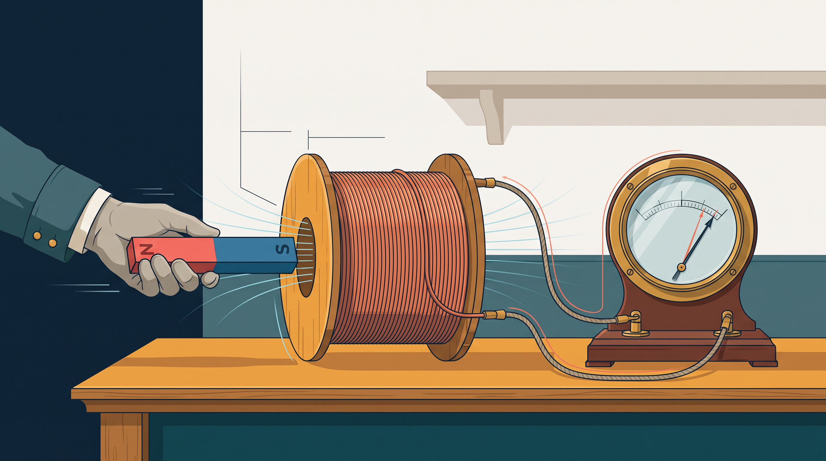
Fig. 6.0 – Faraday’s induction experiment.
By the end of this chapter, you will be able to answer every one of these questions.
6.1 Introduction
For a very long time, people believed that electricity and magnetism were two completely separate things. Electricity was about charges, sparks, and currents. Magnetism was about lodestones and compass needles. Nobody suspected that the two were deeply connected.
This picture changed in the early decades of the nineteenth century. Experiments on electric currents carried out by scientists such as Oersted and Ampere established a striking fact: electricity and magnetism are inter-related. Specifically, they found that moving electric charges produce magnetic fields.
This discovery naturally raises a reverse question. If moving charges (a current) can produce a magnetic field, can the opposite also happen? Can a moving magnet produce an electric current? Does nature permit such a two-way relationship between electricity and magnetism?
The answer is a resounding yes. As you read in the opening story of this chapter, the experiments of Michael Faraday in England and Joseph Henry in the USA, conducted around 1830, settled the matter conclusively. They demonstrated that electric currents were induced in closed coils whenever those coils were subjected to changing magnetic fields.
Notice the key word here: changing. A magnet simply lying near a coil does nothing. It is only when the magnetic field through the coil changes — for example, because the magnet is moving — that a current appears. This single idea is the heart of the entire chapter.
The phenomenon in which an electric current is generated by varying magnetic fields is called electromagnetic induction. The word “induction” is used because the current is not supplied by any battery; it is induced (brought into existence) in the coil by the changing magnetic field. The current produced this way is called an induced current.
Why this discovery matters
Electromagnetic induction is not merely of theoretical or academic interest; it is of enormous practical utility. Imagine a world without electricity — no electric lights, no trains, no telephones, and no personal computers. Almost none of modern life would exist.
The pioneering experiments of Faraday and Henry led directly to the development of the modern-day generator, which converts mechanical energy into electrical energy, and the transformer, which allows electrical energy to be transmitted efficiently across hundreds of kilometres. We will study the generator in detail in Section 6.8 of this chapter.
Today’s civilisation owes its progress, to a great extent, to the discovery of electromagnetic induction. In this chapter, we will study the phenomena associated with changing magnetic fields step by step — first the experiments, then the laws that summarise them, and finally the applications built on those laws.
In board and competitive examinations, this chapter is a favourite source of questions that test whether you can identify what is changing in a given situation — the magnetic field, the area of the loop, or the orientation of the loop. Keep this question in mind throughout: “What is changing here?” It will guide you through every problem on electromagnetic induction.
6.2 The Experiments of Faraday and Henry
Our understanding of electromagnetic induction is built on a long series of careful experiments carried out by Faraday and Henry. Rather than jumping straight to a formula, it is worth walking through some of these experiments, because they show exactly how the induced current behaves and what it depends on. We shall describe three of them.
Before we begin, one small note about vocabulary. Whenever the words “coil” or “loop” are used, we assume they are made of conducting material (usually copper wire) and that the wire is coated with a thin layer of insulating material, so that the current flows along the length of the wire and does not short across neighbouring turns.
Experiment 6.1 — A magnet and a coil
In the first experiment, a coil \(C_1\) is connected to a galvanometer \(G\), as shown in Fig. 6.1. A galvanometer is a sensitive instrument that detects the presence and direction of a small electric current: its pointer deflects one way for current in one direction, and the other way for current in the reverse direction. Importantly, there is no battery in this circuit.
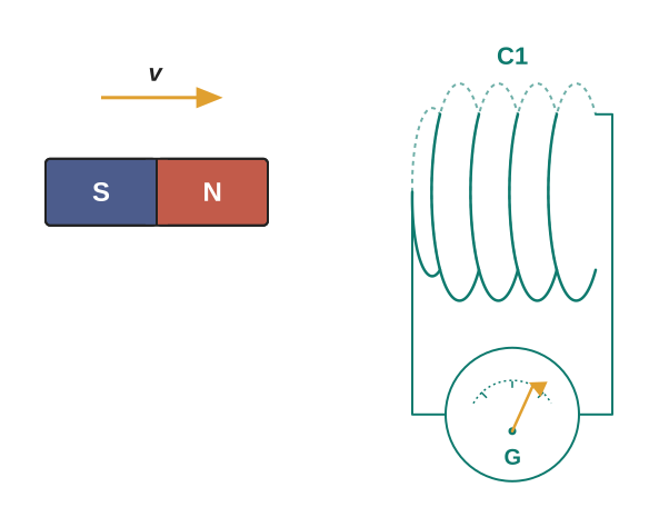
Fig. 6.1 – Current induced by a moving magnet.
When the North-pole of a bar magnet is pushed towards the coil, the galvanometer pointer deflects. This deflection tells us that an electric current has been induced in the coil, even though no battery is present. Crucially, the deflection lasts only as long as the magnet is actually in motion.
The moment the magnet is held stationary — even if it is right next to the coil — the galvanometer shows no deflection at all. This confirms the central idea from Section 6.1: it is the change, not the mere presence of the magnet, that matters.
When the magnet is then pulled away from the coil, the galvanometer deflects in the opposite direction. This tells us the induced current has reversed its direction. So, pushing the magnet in and pulling it out drive the current in opposite senses.
Several more observations sharpen the picture. When the South-pole of the bar magnet (instead of the North-pole) is moved towards or away from the coil, the deflections are opposite to those observed with the North-pole for the same movements. So the polarity of the magnet also decides the direction of the induced current.
The speed of motion matters too. The deflection — and therefore the induced current — is found to be larger when the magnet is pushed towards or pulled away from the coil faster. A quick movement produces a bigger current than a slow one. This hints that the induced effect depends on how rapidly the magnetic situation is changing, an idea we will make precise in Section 6.4.
Finally, a beautiful symmetry appears. If the bar magnet is instead held fixed and the coil \(C_1\) is moved towards or away from the magnet, exactly the same effects are observed. Whether the magnet moves or the coil moves makes no difference to the result.
Experiment 6.2 — Two coils
In the second experiment, the bar magnet is replaced by a second coil \(C_2\) that is connected to a battery, as shown in Fig. 6.2. A steady current flows through \(C_2\) because of the battery, and this steady current produces a steady magnetic field around \(C_2\). In effect, \(C_2\) now behaves like a magnet.
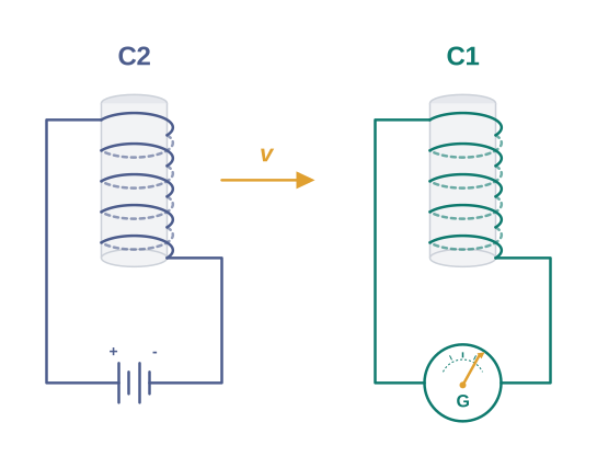
Fig. 6.2 – Current induced by a moving coil.
As coil \(C_2\) is moved towards coil \(C_1\), the galvanometer shows a deflection, indicating that a current is induced in \(C_1\). When \(C_2\) is moved away from \(C_1\), the galvanometer deflects again, but this time in the opposite direction.
Just as before, the deflection lasts only as long as coil \(C_2\) is in motion. And once again, if \(C_2\) is held fixed and \(C_1\) is moved instead, the same effects are seen. The conclusion mirrors Experiment 6.1: it is the relative motion between the two coils that induces the current.
Experiment 6.3 — No motion required
The first two experiments both involved physical movement — of a magnet and a coil, or of two coils. This might tempt us to conclude that motion is essential. Through a third experiment, Faraday showed that this is not true. Relative motion is not an absolute requirement.
Figure 6.3 shows the setup. Two coils \(C_1\) and \(C_2\) are held completely stationary. Coil \(C_1\) is connected to a galvanometer \(G\), while coil \(C_2\) is connected to a battery through a tapping key \(K\) — a simple switch that closes the circuit when pressed and opens it when released.
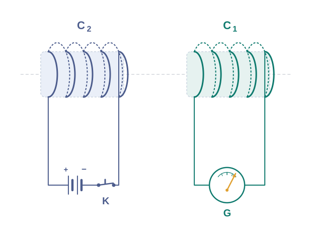
Fig. 6.3 – Current induced by changing a stationary circuit.
The results are revealing. When the tapping key \(K\) is pressed, the galvanometer shows a momentary deflection, and the pointer then returns to zero immediately. If the key is held pressed continuously, there is no deflection at all — a steady current in \(C_2\) produces no induced current in \(C_1\). When the key is released, a momentary deflection is observed once again, but in the opposite direction.
Think about what is happening here. Nothing is moving. Yet at the instant the key is pressed, the current in \(C_2\) (and hence its magnetic field) jumps from zero up to a steady value — a change. At the instant the key is released, the current falls back to zero — again a change. During the in-between period, when the key is held down, the current is steady and unchanging, so no current is induced. The common thread is once more that a changing magnetic field is what induces the current, whether that change is caused by motion or by switching a current on and off.
It is also observed that the deflection increases dramatically when an iron rod is inserted into the coils along their axis. Iron greatly strengthens the magnetic field passing from one coil to the other, so the change in field is much larger, and the induced current is correspondingly bigger. This is why the cores of real transformers and inductors are made of iron.
Taken together, these three experiments point unmistakably to one conclusion, which Faraday captured in a precise mathematical law. But before we can state that law (Section 6.4), we must first make the idea of “magnetic field passing through a coil” quantitative. That measure is called magnetic flux, and it is the subject of the next section.
6.3 Magnetic Flux
Faraday’s great insight was to find a single, simple mathematical relation that could explain all the experiments described in Section 6.2. But before we can state his law, we need a precise way to measure “how much magnetic field passes through a coil.” That measure is called magnetic flux, written \(\Phi_B\).
The idea of magnetic flux is defined in exactly the same way as electric flux was defined in Chapter 1. If you recall, electric flux measured how much electric field passed through a surface. Magnetic flux does the same thing for a magnetic field: it measures how much of the magnetic field “threads through” a given surface.
Flux through a flat surface in a uniform field
Consider a flat plane of area \(A\) placed in a uniform magnetic field \(\mathbf{B}\), as shown in Fig. 6.4. The magnetic flux through this plane is written as
\[\Phi_B = \mathbf{B} \cdot \mathbf{A} = BA \cos\theta \tag{6.1}\]
Here \(B\) is the magnitude of the magnetic field (SI unit: tesla, T), \(A\) is the area of the surface (SI unit: square metre, m²), and \(\theta\) is the angle between the field vector \(\mathbf{B}\) and the area vector \(\mathbf{A}\).
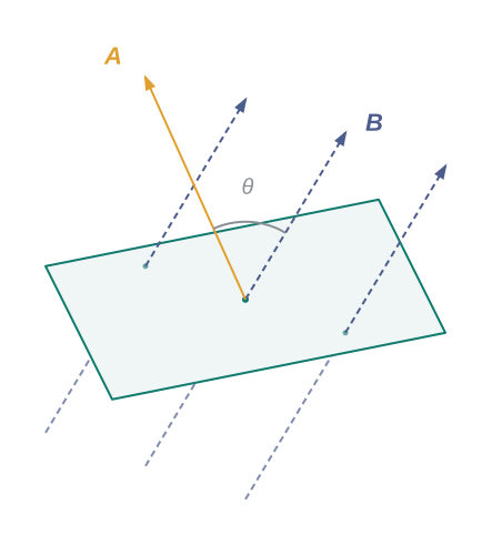
Fig. 6.4 – Magnetic flux through a flat plane.
You may wonder why an area — which sounds like a flat, direction-less quantity — is written as a vector \(\mathbf{A}\). This idea was introduced earlier in Chapter 1. The trick is to represent a surface by a vector whose magnitude equals the area and whose direction points perpendicular (normal) to the surface. This lets us capture not just how big the surface is, but also how it is tilted relative to the field.
The dot product \(\mathbf{B} \cdot \mathbf{A}\) automatically brings in the factor \(\cos\theta\). Let us understand physically why this factor makes sense.
So the flux is greatest when the coil faces the field directly and drops to zero when the coil is turned sideways to the field. This angular dependence will become very important later — in the AC generator (Section 6.8), it is precisely the changing angle \(\theta\) of a rotating coil that produces the induced emf.
Equation (6.1) applies to a flat surface in a uniform field. But it can be extended to curved surfaces and to non-uniform fields as well.
Flux through a curved surface in a non-uniform field
Suppose the magnetic field has different magnitudes and directions at different parts of a surface, as shown in Fig. 6.5. We can no longer use a single value of \(B\) and a single angle \(\theta\) for the whole surface.
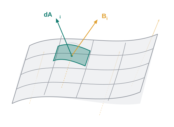
Fig. 6.5 – Magnetic flux through a curved surface.
The way around this is a standard technique in physics: break the surface into a large number of tiny area elements \(d\mathbf{A}_i\). Each element is so small that the field \(\mathbf{B}_i\) over it can be treated as uniform. We compute the flux through each small element as \(\mathbf{B}_i \cdot d\mathbf{A}_i\), and then add up the contributions from all the elements:
\[\Phi_B = \mathbf{B}_1 \cdot d\mathbf{A}_1 + \mathbf{B}_2 \cdot d\mathbf{A}_2 + \cdots = \sum_{\text{all}} \mathbf{B}_i \cdot d\mathbf{A}_i \tag{6.2}\]
Here the label “all” stands for summation over all the area elements \(d\mathbf{A}_i\) that make up the surface, and \(\mathbf{B}_i\) is the magnetic field at the area element \(d\mathbf{A}_i\).
Unit and nature of magnetic flux
The SI unit of magnetic flux is the weber, abbreviated Wb. Since flux is (magnetic field) × (area), it can equivalently be written in terms of tesla and metre: one weber equals one tesla metre squared (T m²). Both are the same unit.
\[1 \text{ Wb} = 1 \text{ T m}^2\]
Finally, an important point about the nature of this quantity: magnetic flux is a scalar quantity. Even though it is built from the two vectors \(\mathbf{B}\) and \(\mathbf{A}\), the dot product between them produces a single number (with a sign), not a direction. So flux has magnitude and sign but no direction of its own.
With the notion of magnetic flux now in hand, we are finally ready to state the law that ties all of Faraday’s experiments together. That is the task of the next section.
6.4 Faraday’s Law of Induction
We now have everything we need to state the law that summarises all of Faraday’s experiments in one clean sentence. From his experimental observations, Faraday arrived at a central conclusion: an emf is induced in a coil whenever the magnetic flux through the coil changes with time.
The term “emf” stands for electromotive force. Despite its name, it is not a force at all — it is the “electrical push” (measured in volts) that drives charges around a circuit. In Faraday’s experiments, it is this induced emf that sets up the induced current we saw deflecting the galvanometer.
Let us first check that this single idea explains all three experiments of Section 6.2.
Re-examining the experiments through flux
In Experiment 6.1, moving a magnet towards or away from coil \(C_1\) changes the magnetic field through the coil, and therefore changes the flux through it. In Experiment 6.2, moving a current-carrying coil \(C_2\) towards or away from \(C_1\) does the same thing. In both cases, it is the change in magnetic flux through \(C_1\) that induces the emf, and this emf drives the current through the galvanometer.
Experiment 6.3 needs a little more thought, because nothing moves there. Here is the explanation. When the tapping key \(K\) is pressed, the current in coil \(C_2\) (and hence its magnetic field) rises from zero to a maximum value in a very short time. Consequently, the magnetic flux through the neighbouring coil \(C_1\) also increases. It is this change in flux through \(C_1\) that produces an induced emf in \(C_1\).
When the key is held pressed, the current in \(C_2\) is constant, so the field is constant, so the flux through \(C_1\) does not change. With no change in flux, the induced emf and current in \(C_1\) drop to zero — exactly as observed.
When the key is released, the current in \(C_2\) and its magnetic field decrease from the maximum value back to zero in a short time. This produces a decrease in the flux through \(C_1\), and hence again induces a current in \(C_1\) — but now in the opposite direction, because the flux is now falling rather than rising.
As a practical caution, note that sensitive electrical instruments placed near an electromagnet can actually be damaged by the induced emfs (and the resulting currents) produced at the instant the electromagnet is switched on or off, because of the sudden change in flux at those moments.
The common point in all these observations is unmistakable: it is the time rate of change of magnetic flux through a circuit that induces an emf in it. Faraday stated this as a formal law.
Statement of Faraday’s law
Mathematically, the induced emf is given by
\[\varepsilon = -\frac{d\Phi_B}{dt} \tag{6.3}\]
Here \(\varepsilon\) is the induced emf (SI unit: volt, V), \(\Phi_B\) is the magnetic flux through the circuit (SI unit: weber, Wb), and \(\dfrac{d\Phi_B}{dt}\) is the rate at which that flux is changing with time (unit: Wb s⁻¹, which is the same as volts).
Notice how neatly this equation captures the earlier observations. A faster movement of the magnet makes \(\dfrac{d\Phi_B}{dt}\) larger, so the induced emf — and hence the deflection — is larger, just as seen in Experiment 6.1. A stationary magnet gives \(\dfrac{d\Phi_B}{dt} = 0\), so there is no emf at all.
The negative sign in Eq. (6.3) is not just decoration. It indicates the direction of the induced emf \(\varepsilon\), and hence the direction of the induced current in a closed loop. This direction rule is important enough to deserve its own treatment, which is why the whole of the next section (Lenz’s law) is devoted to explaining what the negative sign means.
Faraday’s law for a coil of many turns
Most practical coils are not a single loop but are closely wound with many turns of wire. Suppose a coil has \(N\) turns, all wound so closely together that the same flux \(\Phi_B\) links every single turn.
Each turn then experiences the same rate of change of flux, and each turn contributes its own induced emf. Because the turns are joined in series, these emfs simply add up. The total induced emf is therefore \(N\) times the emf of a single turn:
\[\varepsilon = -N\frac{d\Phi_B}{dt} \tag{6.4}\]
Here \(N\) is the number of turns in the coil, and \(\Phi_B\) is the flux linked with each single turn.
This gives us a simple, practical way to boost the induced emf: the induced emf can be increased by increasing the number of turns \(N\) of a closed coil. This is why real coils used in generators and transformers contain hundreds or thousands of turns.
The three ways to change the flux
Equations (6.1) and (6.2) reveal something powerful. Since the flux depends on \(B\), \(A\), and \(\theta\) through \(\Phi_B = BA\cos\theta\), we can change the flux — and hence induce an emf — by changing any one or more of these three quantities.
First, we can change the magnetic field \(\mathbf{B}\). This is exactly what happens in Experiments 6.1 and 6.2, where moving a magnet or a current-carrying coil alters the field through \(C_1\).
Second, we can change the area \(A\) of the coil, for example by shrinking or stretching the loop while it sits in a magnetic field. This changes how much field the loop encloses, and so changes the flux.
Third, we can change the angle \(\theta\) by rotating the coil in the magnetic field, so that the orientation of the coil relative to the field keeps changing. As we will see in Section 6.8, this is exactly how an AC generator works.
In every one of these cases, an emf is induced in the coil. Keeping this three-way classification in mind is extremely useful for solving problems: whenever you face an induction question, first ask which of \(B\), \(A\), or \(\theta\) is changing.
6.5 Lenz’s Law and Conservation of Energy
In Section 6.4 we met Faraday’s law, and we noticed a mysterious negative sign in the equation \(\varepsilon = -\dfrac{d\Phi_B}{dt}\). That sign tells us the direction of the induced emf and current, but it does not, by itself, make the direction obvious. We now unpack what it means, using a wonderfully simple rule discovered shortly after Faraday’s work.
Statement of Lenz’s law
The key word is “opposes.” Nature reacts against the change. If the flux through a coil is increasing, the induced current flows in a direction that tries to decrease it. If the flux is decreasing, the induced current flows in a direction that tries to maintain it. The induced current is always the “resistance” that the circuit puts up against whatever is changing its flux. The negative sign in Eq. (6.3) is simply the mathematical expression of this opposition.
Understanding Lenz’s law through Experiment 6.1
Let us apply the rule to the familiar setup of Experiment 6.1, shown earlier in Fig. 6.1, where the North-pole of a bar magnet is being pushed towards a closed coil.
As the North-pole moves towards the coil, the magnetic flux through the coil increases. By Lenz’s law, the induced current must flow in a direction that opposes this increase. This is possible only if the current in the coil flows in a counter-clockwise direction, as seen by an observer standing on the side of the magnet.
Why counter-clockwise? Because a counter-clockwise current, viewed from the magnet’s side, creates a magnetic moment whose North polarity faces the approaching North-pole of the magnet. Two North-poles facing each other repel. So the coil pushes back against the incoming magnet, opposing its motion — and it is precisely this opposition that resists the increase in flux.
Now consider the reverse. If the North-pole of the magnet is being withdrawn from the coil, the magnetic flux through the coil decreases. To counter this decrease, the induced current now flows in the clockwise direction, so that the coil’s South-pole faces the receding North-pole of the magnet. A North-pole and a South-pole attract, so the coil now pulls on the departing magnet — again opposing the motion, and this time opposing the decrease in flux.
In both cases, the induced current opposes the change, exactly as Lenz’s law demands. Notice that the coil never “helps” the magnet; it always fights whatever the magnet is trying to do.
Lenz’s law for an open circuit
What happens if we use an open circuit instead of a closed loop in the above example? Since the circuit is broken, no continuous current can flow. But an emf is still induced across the open ends of the circuit — the “push” is present even if the charges cannot complete a loop.
The direction (polarity) of this induced emf can still be found using Lenz’s law. Figures 6.6(a) and (b) provide an easier way to picture the direction of the induced currents in such situations.
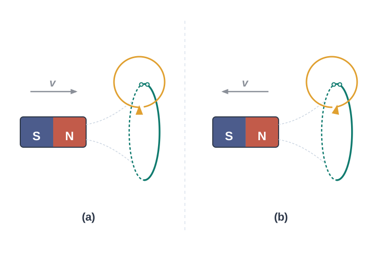
Fig. 6.6 – Direction of induced current and Lenz’s law.
The curved arrows drawn in the figure indicate the directions of the induced currents that would flow if the circuit were closed, and thus tell us the polarity of the induced emf across the open ends.
Lenz’s law as a consequence of energy conservation
Lenz’s law is not just a convenient recipe for finding directions — it is a direct consequence of the law of conservation of energy. A little reflection shows why the induced current must oppose the change, and could not possibly do the reverse.
Suppose, for the sake of argument, that the induced current were in the opposite direction to the one shown in Fig. 6.6(a). Then the South-pole due to the induced current would face the approaching North-pole of the magnet. These opposite poles would attract, so the magnet would be pulled towards the coil with an ever-increasing acceleration.
Follow this to its conclusion. A single gentle push would set the magnet moving, and from then on the attraction would keep speeding it up. Its velocity and kinetic energy would go on increasing without any energy being supplied from outside. If this could happen, one could build a perpetual-motion machine — a device that produces energy from nothing. This clearly violates the law of conservation of energy, and so it cannot happen. The induced current is therefore forced to oppose, not assist, the motion.
Where does the energy go?
Now consider the correct case, shown in Fig. 6.6(a). Here the bar magnet experiences a repulsive force due to the induced current, so a person must do work to push the magnet against this repulsion.
That work does not vanish. The energy spent by the person is converted, through the induced current, into heat inside the coil. This heating, caused by the resistance of the coil, is called Joule heating. In short, the mechanical energy you put in to move the magnet reappears as electrical energy in the current and finally as heat in the wire — energy is conserved at every step.
This energy accounting is the deep reason electromagnetic induction can power our world: a generator does not create energy, it converts the mechanical energy of a spinning turbine into electrical energy, exactly as a person’s pushing work is converted here.
Figure 6.7 shows planar loops of different shapes moving out of, or into, a region of a magnetic field which is directed normal to the plane of the loop and away from the reader. Determine the direction of the induced current in each loop using Lenz’s law.
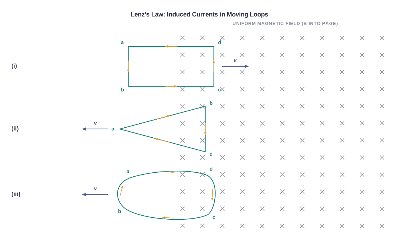
[Caption:] Fig. 6.7 – Induced currents in loops moving through a magnetic field. [/Caption:]
Solution
The field points into the page (away from the reader), shown by the crosses. In each case we ask: is the flux into the page increasing or decreasing, and which way must the induced current flow to oppose that?
The magnetic flux through the rectangular loop \(abcd\) increases, because the loop is moving into the region of magnetic field and enclosing more of it. To oppose this increase, the induced current must set up a field out of the page inside the loop, which requires it to flow along the path \(bcdab\).
Due to the outward motion, the magnetic flux through the triangular loop \(abc\) decreases, since less of the field is enclosed. To oppose this decrease, the induced current flows along \(bacb\), so as to maintain the flux.
As the magnetic flux decreases due to the motion of the irregular-shaped loop \(abcd\) out of the field region, the induced current flows along \(cdabc\), again opposing the change in flux.
Note that there is no induced current as long as the loops are completely inside or completely outside the region of the magnetic field. In those situations the enclosed flux is not changing, so nothing is induced. A current appears only while a loop is crossing the boundary of the field region.
(a) A closed loop is held stationary in the magnetic field between the north and south poles of two permanent magnets held fixed. Can we hope to generate a current in the loop by using very strong magnets?
(b) A closed loop moves normal to the constant electric field between the plates of a large capacitor. Is a current induced in the loop (i) when it is wholly inside the region between the capacitor plates, and (ii) when it is partially outside the plates of the capacitor? The electric field is normal to the plane of the loop.
(c) A rectangular loop and a circular loop are moving out of a uniform magnetic field region (Fig. 6.8) to a field-free region with a constant velocity \(\mathbf{v}\). In which loop do you expect the induced emf to be constant during the passage out of the field region? The field is normal to the loops.
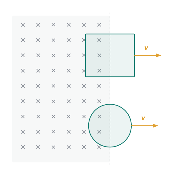
[Caption:] Fig. 6.8 – Rectangular and circular loops leaving a magnetic field. [/Caption:]
(d) Predict the polarity of the capacitor in the situation described by Fig. 6.9.
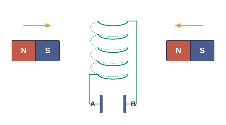
[Caption:] Fig. 6.9 – Magnets approaching a coil-capacitor circuit. [/Caption:]
Solution
No. However strong the magnet may be, a current can be induced only by changing the magnetic flux through the loop. Here the loop is stationary and the field is steady, so the flux does not change, and no current is generated. Strength of the magnet is irrelevant.
No current is induced in either case. Electromagnetic induction responds only to a change in magnetic flux. A current cannot be induced by changing the electric flux, so neither position of the loop produces a current.
The induced emf is expected to be constant only in the case of the rectangular loop. As the rectangular loop leaves the field, the length of its boundary crossing the field edge stays the same, so the rate of change of area (and hence flux) is constant. For the circular loop, the rate of change of area of the loop during its passage out of the field region is not constant — the width of the circle at the boundary keeps changing — hence the induced emf will vary accordingly.
The polarity of plate ‘A’ will be positive with respect to plate ‘B’ in the capacitor.
6.6 Motional Electromotive Force
So far, most of our examples have produced an induced emf by changing the magnetic field. But recall from Section 6.4 that flux can also be changed by changing the area of a circuit. In this section we explore that route, and in doing so we discover a second, complementary way of understanding induction — one based directly on the force felt by moving charges. This will also answer the question of where the emf across a moving rod comes from.
Induced emf from a changing area
Let us consider a straight conductor moving in a uniform and time-independent magnetic field. Figure 6.10 shows a rectangular conductor \(PQRS\) in which the arm \(PQ\) is free to slide. The rod \(PQ\) is moved towards the left with a constant velocity \(\mathbf{v}\), as shown. We assume there is no loss of energy due to friction.
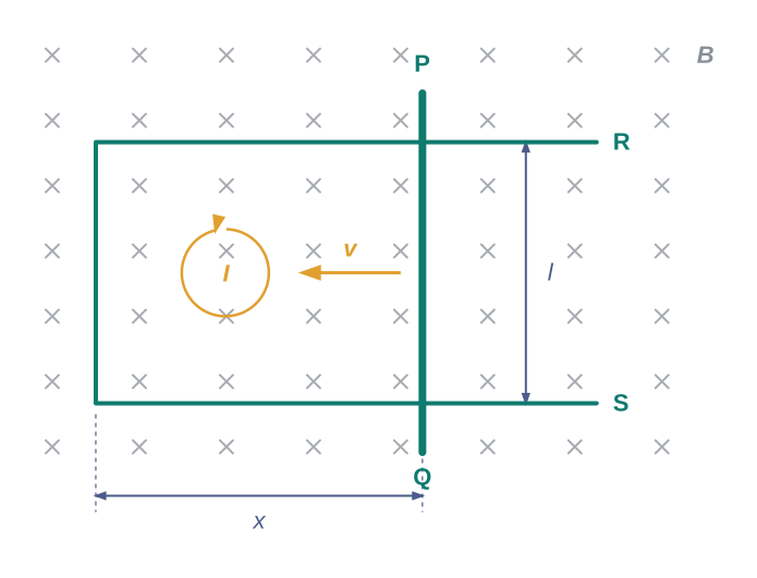
Fig. 6.10 – Motional emf in a sliding rod.
The four arms \(PQRS\) together form a closed circuit, enclosing an area that changes as \(PQ\) slides. The whole arrangement is placed in a uniform magnetic field \(\mathbf{B}\) perpendicular to the plane of the system. Let the length \(RQ = x\) and \(RS = l\). Then the area enclosed is \(lx\), and the magnetic flux \(\Phi_B\) through the loop \(PQRS\) is
\[\Phi_B = Blx\]
Here \(B\) is the magnetic field magnitude, \(l\) is the fixed length of the sliding rod, and \(x\) is the distance that changes as the rod moves.
Since \(x\) is changing with time, the flux \(\Phi_B\) is changing too, and by Faraday’s law this changing flux induces an emf. Differentiating with respect to time:
\[\varepsilon = -\frac{d\Phi_B}{dt} = -\frac{d}{dt}(Blx) = -Bl\frac{dx}{dt} = Blv \tag{6.5}\]
In the last step we used \(\dfrac{dx}{dt} = -v\), where \(v\) is the speed of the conductor \(PQ\) (the sign is negative because \(x\) decreases as the rod moves left, reducing the area). The two negative signs cancel, leaving a positive result.
The induced emf \(Blv\) is called the motional emf, because it is produced by the motion of the conductor rather than by any change in the magnetic field itself.
Here \(\varepsilon\) is the emf in volts, \(B\) is the field in tesla, \(l\) is the length of the rod in metres, and \(v\) is its speed in metres per second. This result shows that we can produce an induced emf simply by moving a conductor — that is, by changing the magnetic flux enclosed by the circuit — without ever varying the magnetic field.
The same result from the Lorentz force
There is a second, more physical way to arrive at the motional emf of Eq. (6.5), one that does not mention flux at all. It uses the Lorentz force acting on the free charge carriers inside the moving conductor \(PQ\). This second view is important because it reveals where the emf actually comes from at the level of individual charges.
Recall from the earlier chapter on magnetism that a charge \(q\) moving with velocity \(\mathbf{v}\) in a magnetic field \(\mathbf{B}\) experiences a magnetic force. Consider any arbitrary charge \(q\) inside the conductor \(PQ\). When the rod moves with speed \(v\), this charge is carried along with speed \(v\) through the magnetic field \(\mathbf{B}\).
The magnetic (Lorentz) force on this charge has magnitude \(qvB\), and its direction is along the rod, towards the end \(Q\). Every free charge in the rod feels the same force, in the same direction, regardless of where it sits along the rod. This force pushes the positive charges towards \(Q\), setting up the emf.
The work done in moving the charge from end \(P\) to end \(Q\), a distance \(l\), is force times distance:
\[W = qvBl\]
Now, emf is defined as the work done per unit charge in driving charge around the circuit. So
\[\varepsilon = \frac{W}{q} = Blv\]
This equation gives the emf induced across the rod \(PQ\), and it is identical to Eq. (6.5) obtained from Faraday’s law. We should be honest that this charge-based argument is not wholly rigorous, but it does help us understand the physical basis of Faraday’s law when a conductor moves in a uniform, time-independent magnetic field. The emf comes from the magnetic force herding the free charges to one end of the rod.
Two views, and the deeper meaning
The two derivations describe two different physical situations that happen to give the same formula. When the conductor moves and the field is steady, the emf can be traced to the magnetic Lorentz force on the moving charges, as we just saw.
But now consider the opposite situation: the conductor is stationary and the magnetic field is changing (as in Experiment 6.3). It is not at all obvious how an emf arises here — yet Faraday verified by numerous experiments that it does. For a stationary conductor, the force on its charges is given by the full Lorentz expression
\[\mathbf{F} = q(\mathbf{E} + \mathbf{v} \times \mathbf{B}) = q\mathbf{E} \tag{6.6}\]
since \(\mathbf{v} = 0\) for the stationary charges, which kills the magnetic term \(q(\mathbf{v} \times \mathbf{B})\). Thus, any force on the charge must come from the electric field term \(\mathbf{E}\) alone.
This forces a remarkable conclusion. To explain the existence of an induced emf in a stationary conductor, we must assume that a time-varying magnetic field generates an electric field. A changing magnetic field creates an electric field that pushes the charges around — this is something genuinely new.
We should add, however, that electric fields produced by static charges have properties different from those produced by time-varying magnetic fields. They are not identical kinds of electric field, even though both exert force \(q\mathbf{E}\) on charges.
Step back and admire the symmetry. In the earlier chapter you learnt that charges in motion (a current) can exert a force or torque on a stationary magnet. Now we find the converse: a bar magnet in motion — or more generally, any changing magnetic field — can exert a force on a stationary charge. This is the fundamental significance of Faraday’s discovery: electricity and magnetism are two aspects of one unified phenomenon. They are truly related.
A metallic rod of 1 m length is rotated with a frequency of 50 rev/s, with one end hinged at the centre and the other end at the circumference of a circular metallic ring of radius 1 m, about an axis passing through the centre and perpendicular to the plane of the ring (Fig. 6.11). A constant and uniform magnetic field of 1 T parallel to the axis is present everywhere. What is the emf between the centre and the metallic ring?
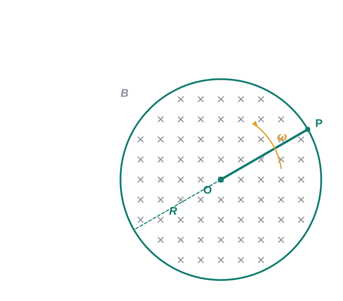
[Caption:] Fig. 6.11 – Motional emf in a rotating rod. [/Caption:]
Solution
Method I. As the rod is rotated, the free electrons in the rod are pushed towards the outer end by the Lorentz force, and get distributed over the ring. This separation of charges produces an emf across the ends of the rod. At a certain value of emf, there is no more flow of electrons and a steady state is reached.
The trick here is that different parts of the rod move at different speeds — a point at distance \(r\) from the centre moves with speed \(v = \omega r\). So we cannot use \(Blv\) with a single \(v\). Instead, using Eq. (6.5), the emf generated across a small length \(dr\) of the rod, as it moves at right angles to the field, is
\[d\varepsilon = Bv\,dr\]
To get the total emf, we add up (integrate) the contributions from all the little pieces from the centre (\(r = 0\)) to the rim (\(r = R\)):
\[\varepsilon = \int d\varepsilon = \int_0^R Bv\,dr = \int_0^R B\omega r\,dr = \frac{B\omega R^2}{2}\]
Note that we used \(v = \omega r\). Substituting the numbers, with \(\omega = 2\pi \times (\text{frequency}) = 2\pi \times 50\):
\[\varepsilon = \frac{1}{2} \times 1.0 \times 2\pi \times 50 \times (1^2) = 157 \text{ V}\]
Method II. We can also calculate the emf using rate of change of area. Imagine a closed loop \(OPQ\) in which point \(O\) and point \(P\) are connected by a resistor \(R\), and \(OQ\) is the rotating rod. The potential difference across the resistor then equals the induced emf, which equals \(B \times\) (rate of change of area of the loop).
If \(\theta\) is the angle between the rod and the reference radius at \(P\) at time \(t\), the area of the sector \(OPQ\) is
\[\pi R^2 \times \frac{\theta}{2\pi} = \frac{1}{2}R^2\theta\]
where \(R\) is the radius of the circle. Hence the induced emf is
\[\varepsilon = B \times \frac{d}{dt}\left[\frac{1}{2}R^2\theta\right] = \frac{1}{2}BR^2\frac{d\theta}{dt} = \frac{B\omega R^2}{2}\]
where we used \(\dfrac{d\theta}{dt} = \omega = 2\pi\nu\). This expression is identical to the one obtained by Method I, and gives the same value of \(\varepsilon\).
6.7 Inductance
We have seen two ways to induce a current in a coil: by changing the magnetic field near it, and by moving a conductor. There is a third, very practical situation that appears again and again in real circuits — the current induced by a changing current. This can happen in two ways: the changing current may be in a neighbouring coil, or it may be in the same coil. Both are governed by a single property called inductance, which is the subject of this section.
An electric current can be induced in a coil by a flux change produced by another coil in its vicinity, or by a flux change produced by the same coil. These two situations are described separately in the next two sub-sections. However, in both cases there is one common starting point: the magnetic flux through a coil is proportional to the current producing it. That is,
\[\Phi_B \propto I\]
This makes physical sense: double the current and you double the magnetic field, and hence double the flux. Further, provided the geometry of the coil does not change with time, this proportionality carries over to the rates of change:
\[\frac{d\Phi_B}{dt} \propto \frac{dI}{dt}\]
Flux linkage
For a closely wound coil of \(N\) turns, the same magnetic flux \(\Phi_B\) links every one of the turns. When the flux \(\Phi_B\) through the coil changes, each turn contributes to the induced emf, so what matters is the total flux threading all the turns together.
To capture this, we define a quantity called flux linkage, equal to \(N\Phi_B\) for a closely wound coil. In terms of flux linkage, the proportionality with current becomes
\[N\Phi_B \propto I\]
The constant of proportionality in this relation is called the inductance.
What inductance depends on
We shall see, in the two sub-sections below, that inductance depends only on the geometry of the coil (its size, shape, and number of turns) and on the intrinsic magnetic properties of the material inside it. It does not depend on the current flowing.
This aspect is closely similar to capacitance, which you met in an earlier chapter. The capacitance of a parallel plate capacitor depends on the plate area and plate separation (its geometry) and on the dielectric constant \(K\) of the medium between the plates (an intrinsic material property). Inductance plays an analogous role for coils.
Inductance is a scalar quantity. It has the dimensions of \([\text{M L}^2 \text{T}^{-2} \text{A}^{-2}]\), obtained by dividing the dimensions of flux by the dimensions of current. The SI unit of inductance is the henry, denoted by H. It is named in honour of Joseph Henry, who discovered electromagnetic induction in the USA independently of Faraday in England.
6.7.1 Mutual inductance
We begin with the case of two coils, where a changing current in one coil induces an emf in the other. Consider Fig. 6.12, which shows two long co-axial solenoids, each of length \(l\) — that is, two long cylindrical coils sharing the same central axis, one nested inside the other.
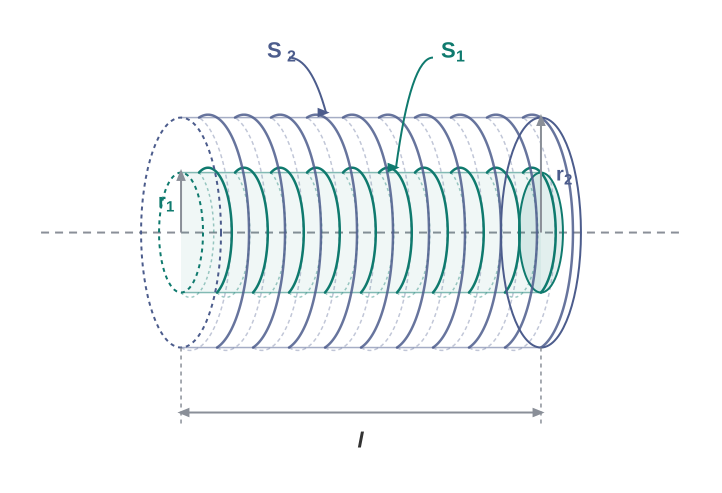
Fig. 6.12 – Two long co-axial solenoids.
Let us set up the notation carefully. We denote the radius of the inner solenoid \(S_1\) by \(r_1\) and its number of turns per unit length by \(n_1\). The corresponding quantities for the outer solenoid \(S_2\) are \(r_2\) and \(n_2\). Let \(N_1\) and \(N_2\) be the total number of turns of coils \(S_1\) and \(S_2\), respectively. (Since turns-per-unit-length times length gives total turns, \(N_1 = n_1 l\) and \(N_2 = n_2 l\).)
Current in the outer solenoid. When a current \(I_2\) is set up through \(S_2\), it in turn sets up a magnetic flux through \(S_1\). Let us denote this flux by \(\Phi_1\). The corresponding flux linkage with solenoid \(S_1\) is written as
\[N_1\Phi_1 = M_{12}I_2 \tag{6.7}\]
Here \(M_{12}\) is called the mutual inductance of solenoid \(S_1\) with respect to solenoid \(S_2\). It is also referred to as the coefficient of mutual induction. The subscript order “\(1\,2\)” reads as “the effect on coil 1 due to coil 2.”
For these simple co-axial solenoids, it is possible to calculate \(M_{12}\) explicitly. The magnetic field inside a long solenoid \(S_2\) carrying current \(I_2\) is \(\mu_0 n_2 I_2\), directed along the axis. Since the inner solenoid \(S_1\) lies entirely within this field, the flux through each turn of \(S_1\) is this field times the cross-sectional area \(\pi r_1^2\) of \(S_1\). The resulting flux linkage with coil \(S_1\) (which has \(n_1 l\) turns) is
\[N_1\Phi_1 = (n_1 l)\left(\pi r_1^2\right)\left(\mu_0 n_2 I_2\right) = \mu_0 n_1 n_2 \pi r_1^2 l\, I_2 \tag{6.8}\]
where \(n_1 l\) is the total number of turns in solenoid \(S_1\). Comparing Eq. (6.8) with Eq. (6.7), we can read off the mutual inductance:
\[M_{12} = \mu_0 n_1 n_2 \pi r_1^2 l \tag{6.9}\]
Notice that we neglected the edge effects and treated the field \(\mu_0 n_2 I_2\) as uniform throughout the length and width of the solenoid \(S_2\). This is a good approximation, kept valid by the solenoid being long, meaning \(l \gg r_2\). (Near the open ends of a real solenoid the field spreads and weakens, but for a long solenoid these ends are a negligible fraction of the whole.)
Current in the inner solenoid — the reverse case. Now we do the reverse: pass a current \(I_1\) through the inner solenoid \(S_1\) and find the flux linkage with the outer coil \(S_2\). This is written as
\[N_2\Phi_2 = M_{21}I_1 \tag{6.10}\]
where \(M_{21}\) is the mutual inductance of solenoid \(S_2\) with respect to solenoid \(S_1\).
The flux due to the current \(I_1\) in \(S_1\) can be assumed to be confined solely inside \(S_1\), since the solenoids are very long and the inner solenoid’s field is negligible outside it. Thus the flux linkage with solenoid \(S_2\) (which has \(n_2 l\) turns) is
\[N_2\Phi_2 = (n_2 l)\left(\pi r_1^2\right)\left(\mu_0 n_1 I_1\right)\]
Note that the relevant area here is still \(\pi r_1^2\), the cross-section of the inner solenoid, because the inner solenoid’s field exists only within its own cross-section. From Eq. (6.10),
\[M_{21} = \mu_0 n_1 n_2 \pi r_1^2 l \tag{6.11}\]
The equality of the two mutual inductances. Comparing Eq. (6.9) and Eq. (6.11), we find the two coefficients are exactly equal:
\[M_{12} = M_{21} = M \text{ (say)} \tag{6.12}\]
We have demonstrated this equality only for long co-axial solenoids, but the relation is far more general and holds for any pair of coils. This generality is more than a curiosity — it is genuinely useful. Suppose the inner solenoid were much shorter than the outer one, and placed well inside it. We could still easily calculate the flux linkage \(N_1\Phi_1\), because the inner solenoid would be sitting in the uniform field of the outer solenoid; so finding \(M_{12}\) would be easy.
However, it would be extremely difficult to calculate the flux linkage with the outer solenoid directly, because the field due to the short inner solenoid would vary across both the length and the cross-section of the outer solenoid. So calculating \(M_{21}\) directly would be very hard. The equality \(M_{12} = M_{21}\) rescues us: we compute the easy one and simply set the hard one equal to it.
Effect of a magnetic medium. We explained the above with air (or vacuum) as the medium within the solenoids. Instead, if a medium of relative permeability \(\mu_r\) had been present, the mutual inductance would be
\[M = \mu_r \mu_0 n_1 n_2 \pi r_1^2 l\]
This is why inserting an iron core (which has a large \(\mu_r\)) so dramatically increases the coupling between coils — exactly the dramatic increase in deflection we saw when an iron rod was inserted in Experiment 6.3.
It is also important to know that the mutual inductance of a pair of coils, solenoids, and so on, depends on their separation as well as their relative orientation. Move the coils apart, or tilt one relative to the other, and \(M\) changes.
Induced emf from mutual inductance. Now let us recollect Experiment 6.3 in Section 6.2. In that experiment, an emf was induced in coil \(C_1\) whenever there was any change in the current through coil \(C_2\). We can now describe this precisely. Let \(\Phi_1\) be the flux through coil \(C_1\) (say of \(N_1\) turns) when the current in coil \(C_2\) is \(I_2\).
Then, from Eq. (6.7), we have
\[N_1\Phi_1 = MI_2\]
For currents varying with time, we differentiate both sides:
\[\frac{d(N_1\Phi_1)}{dt} = \frac{d(MI_2)}{dt}\]
Since the induced emf in coil \(C_1\) is given by Faraday’s law, \(\varepsilon_1 = -\dfrac{d(N_1\Phi_1)}{dt}\), and since \(M\) is a constant, we get
\[\varepsilon_1 = -M\frac{dI_2}{dt}\]
This shows that varying the current in a coil can induce an emf in a neighbouring coil. The magnitude of the induced emf depends on the rate of change of current, \(\dfrac{dI_2}{dt}\), and on the mutual inductance \(M\) of the two coils.
6.7.2 Self-inductance
In the previous sub-section, we considered the flux in one solenoid due to the current in another. It is also possible for an emf to be induced in a single isolated coil, due to a change of flux through that same coil caused by varying the current through it. This phenomenon is called self-induction. In everyday terms, a coil reacts against changes in its own current.
In this case, the flux linkage through a coil of \(N\) turns is proportional to the current through the coil itself, and is expressed as
\[N\Phi_B \propto I\] \[N\Phi_B = LI \tag{6.13}\]
where the constant of proportionality \(L\) is called the self-inductance of the coil. It is also called the coefficient of self-induction of the coil.
When the current is varied, the flux linked with the coil also changes, and by Faraday’s law an emf is induced in the coil. Using Eq. (6.13), the induced emf is
\[\varepsilon = -\frac{d(N\Phi_B)}{dt}\] \[\varepsilon = -L\frac{dI}{dt} \tag{6.14}\]
The negative sign here is Lenz’s law in action. It tells us that the self-induced emf always opposes any change — increase or decrease — of the current in the coil. If you try to increase the current, the coil pushes back to slow the increase; if you try to decrease it, the coil pushes to keep the current going.
Self-inductance of a long solenoid
It is possible to calculate the self-inductance for circuits with simple geometries. Let us calculate the self-inductance of a long solenoid of cross-sectional area \(A\) and length \(l\), having \(n\) turns per unit length.
The magnetic field due to a current \(I\) flowing in the solenoid is \(B = \mu_0 n I\) (again neglecting edge effects, as before). The total flux linked with the solenoid is the flux per turn times the total number of turns \(nl\):
\[N\Phi_B = (nl)(\mu_0 n I)(A) = \mu_0 n^2 A l\, I\]
where \(nl\) is the total number of turns. Thus, using the definition \(L = N\Phi_B / I\) from Eq. (6.13), the self-inductance is
\[L = \frac{N\Phi_B}{I} = \mu_0 n^2 A l \tag{6.15}\]
Notice, as promised, that \(L\) depends only on the geometry — the turns per unit length \(n\), the area \(A\), and the length \(l\) — and not on the current.
If we fill the inside of the solenoid with a material of relative permeability \(\mu_r\) (for example soft iron, which has a high value of relative permeability), then
\[L = \mu_r \mu_0 n^2 A l \tag{6.16}\]
So the self-inductance of the coil depends on its geometry and on the permeability of the medium inside it. An iron core can raise \(L\) by a large factor.
Self-inductance as electrical inertia
The self-induced emf is also called the back emf, because it acts back against any change in the current in a circuit. Physically, the self-inductance plays the role of inertia. It is the electromagnetic analogue of mass in mechanics: just as mass resists changes in the motion of an object, self-inductance resists changes in the current.
Because the coil opposes the build-up of current with a back emf, work must be done against this back emf \(\varepsilon\) to establish the current. This work done is stored as magnetic potential energy in the coil. Let us calculate how much.
For a current \(I\) at an instant in the circuit, the rate of work done against the back emf is
\[\frac{dW}{dt} = |\varepsilon| I\]
If we ignore the resistive losses and consider only the inductive effect, then using Eq. (6.14) (with \(|\varepsilon| = L\,dI/dt\)),
\[\frac{dW}{dt} = L\,I\frac{dI}{dt}\]
The total amount of work done in establishing the current from \(0\) to \(I\) is found by integrating:
\[W = \int dW = \int_0^I L\,I\,dI\]
Thus, the energy required to build up the current \(I\) is
\[W = \frac{1}{2}LI^2 \tag{6.17}\]
This expression is worth pausing on. It reminds us strongly of \(\tfrac{1}{2}mv^2\) for the mechanical kinetic energy of a particle of mass \(m\). Comparing the two, we see that \(L\) is analogous to \(m\): that is, \(L\) is a kind of electrical inertia that opposes the growth and decay of current in the circuit, exactly as mass opposes changes in velocity.
The general case of two coupled coils
Consider the general case of currents flowing simultaneously in two nearby coils. The flux linked with one coil will be the sum of two contributions — one due to its own current, and one due to the current in the other coil, which exist independently and add up.
Equation (6.7) is therefore modified into
\[N_1\Phi_1 = M_{11}I_1 + M_{12}I_2\]
where \(M_{11}\) represents the inductance due to the coil’s own current (a “self” term), and \(M_{12}\) the mutual coupling to the second coil. Therefore, using Faraday’s law,
\[\varepsilon_1 = -M_{11}\frac{dI_1}{dt} - M_{12}\frac{dI_2}{dt}\]
Now, \(M_{11}\) is simply the self-inductance of coil 1, and is conventionally written as \(L_1\). Therefore,
\[\varepsilon_1 = -L_1\frac{dI_1}{dt} - M_{12}\frac{dI_2}{dt}\]
So the emf in coil 1 has two parts: one from the change in its own current (self-inductance) and one from the change in the neighbouring current (mutual inductance). This is the complete description of two magnetically coupled coils.
6.8 AC Generator
We have now built up all the principles of electromagnetic induction. It is time to see them come together in the single most important application of the whole subject — the device that generates almost all the electricity used in the world.
The phenomenon of electromagnetic induction has been technologically exploited in many ways. An exceptionally important application is the generation of alternating currents (AC). The modern AC generator, with a typical output capacity of 100 MW, is a highly evolved machine. In this section we describe the basic principles behind it. The Yugoslav-born inventor Nikola Tesla is credited with the development of this machine.
The principle: changing the flux by rotation
Recall from Section 6.4 that one way to induce an emf in a loop is through a change in the loop’s orientation, or equivalently a change in its effective area facing the field. The AC generator uses exactly this idea.
As a coil rotates in a magnetic field \(\mathbf{B}\), the effective area of the loop — meaning the face perpendicular to the field — is \(A\cos\theta\), where \(\theta\) is the angle between the area vector \(\mathbf{A}\) and the field \(\mathbf{B}\). As the coil turns, \(\theta\) keeps changing, so the effective area keeps changing, so the flux keeps changing, and an emf is continuously induced. This method of producing a flux change is the principle of operation of a simple AC generator.
The basic construction
The basic elements of an AC generator are shown in Fig. 6.13. It consists of a coil mounted on a rotor shaft, with the axis of rotation of the coil perpendicular to the direction of the magnetic field.
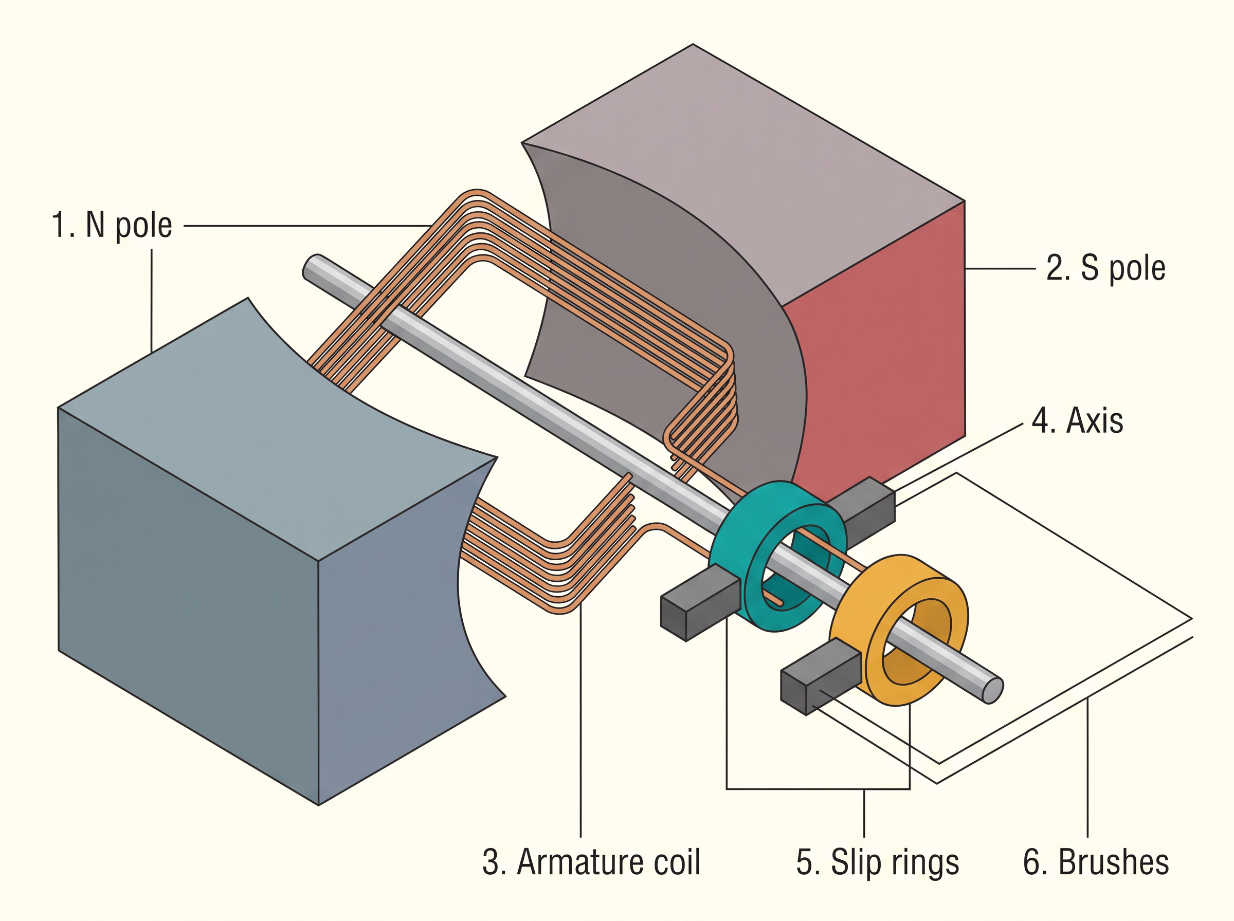
Fig. 6.13 – Basic components of an AC generator.
The coil, called the armature, is mechanically rotated in the uniform magnetic field by some external means — a turbine, an engine, or hand-cranking. As the coil rotates, the magnetic flux through it changes, and so an emf is induced in the coil.
The two ends of the coil cannot simply be soldered to fixed wires, because the coil is spinning. Instead, they are connected to the external circuit by means of slip rings and carbon brushes. The slip rings rotate with the coil, while the stationary carbon brushes press against them and carry the current out to the external circuit. This clever arrangement lets a spinning coil feed a stationary circuit.
Deriving the alternating emf
Let the coil be rotated with a constant angular speed \(\omega\). The angle \(\theta\) between the magnetic field vector \(\mathbf{B}\) and the area vector \(\mathbf{A}\) of the coil at any instant \(t\) is \(\theta = \omega t\) (assuming \(\theta = 0°\) at \(t = 0\)). As a result, the effective area of the coil exposed to the field lines changes with time, and from Eq. (6.1) the flux at any time \(t\) is
\[\Phi_B = BA\cos\theta = BA\cos\omega t\]
From Faraday’s law, the induced emf for the rotating coil of \(N\) turns is then
\[\varepsilon = -N\frac{d\Phi_B}{dt} = -NBA\frac{d}{dt}(\cos\omega t)\]
Differentiating \(\cos\omega t\) gives \(-\omega\sin\omega t\), and the two negative signs cancel. Thus the instantaneous value of the emf is
\[\varepsilon = NBA\,\omega\sin\omega t \tag{6.19}\]
Here \(N\) is the number of turns, \(B\) the field, \(A\) the coil area, \(\omega\) the angular speed, and \(t\) the time.
The quantity \(NBA\omega\) is the maximum value of the emf, which occurs when \(\sin\omega t = \pm 1\). If we denote \(NBA\omega\) by the symbol \(\varepsilon_0\), then
\[\varepsilon = \varepsilon_0 \sin\omega t \tag{6.20}\]
Why it is called alternating
Since the value of the sine function varies between \(+1\) and \(-1\), the sign — that is, the polarity — of the emf changes periodically with time. Note from Fig. 6.14 that the emf has its extreme value when \(\theta = 90°\) or \(\theta = 270°\), because the change of flux is greatest at these points.
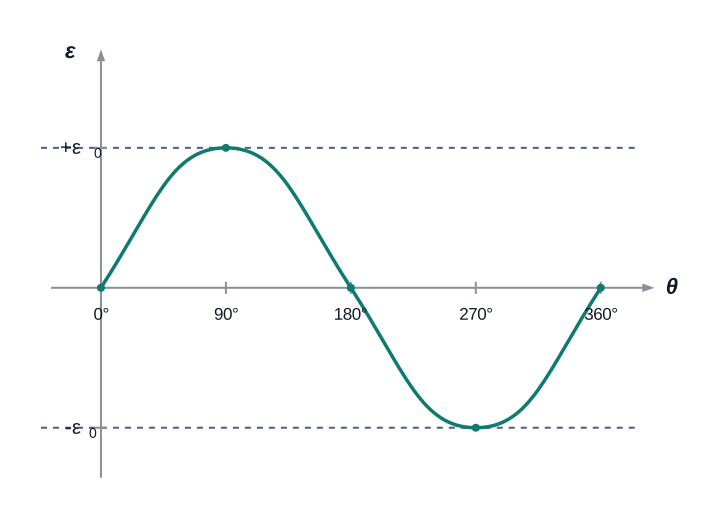
Fig. 6.14 – Alternating emf generated by a rotating coil.
Because the polarity keeps reversing, the direction of the current in the external circuit also changes periodically. A current whose direction reverses regularly like this is called alternating current (AC). Since \(\omega = 2\pi\nu\), Eq. (6.20) can also be written in terms of the frequency of revolution \(\nu\):
\[\varepsilon = \varepsilon_0 \sin 2\pi\nu t \tag{6.21}\]
where \(\nu\) is the frequency of revolution of the generator’s coil.
Note that Eq. (6.20) and Eq. (6.21) give the instantaneous value of the emf, and that \(\varepsilon\) varies between \(+\varepsilon_0\) and \(-\varepsilon_0\) periodically. In the next chapter you will learn how to determine the time-averaged value for such an alternating voltage and current, since a quantity that keeps swinging positive and negative needs a careful definition of its “average” size.
Real generators
In commercial generators, the mechanical energy required for the rotation of the armature comes from different sources. In some, it is provided by water falling from a height, for example from dams; these are called hydro-electric generators. In others, water is heated to produce steam using coal or other fuels, and the high-pressure steam rotates the armature; these are called thermal generators. If a nuclear fuel is used to produce the heat instead of coal, we get nuclear power generators.
Modern-day generators produce electric power as high as 500 MW — enough to light up 5 million bulbs of 100 W each. In most large generators, a practical reversal is used: the coils are held stationary and it is the electromagnets that are rotated, which is mechanically easier for such huge machines. The frequency of rotation is 50 Hz in India, while in certain countries such as the USA it is 60 Hz.
6.9 Summary
This summary gathers the key results of the chapter in one place. Each point restates a law or formula you met in the sections above, so you can use it for quick revision.
- Magnetic flux. The magnetic flux through a surface of area \(A\) placed in a uniform magnetic field \(B\) is defined as
\[\Phi_B = \mathbf{B}\cdot\mathbf{A} = BA\cos\theta\]
where \(\theta\) is the angle between \(\mathbf{B}\) and \(\mathbf{A}\) (the area vector). Flux is a scalar, measured in weber (Wb).
- Faraday’s law of induction. Faraday’s laws imply that the emf induced in a coil of \(N\) turns is directly related to the rate of change of flux through it:
\[\varepsilon = -N\frac{d\Phi_B}{dt}\]
Here \(\Phi_B\) is the flux linked with one turn of the coil. If the circuit is closed, a current \(I = \varepsilon/R\) is set up in it, where \(R\) is the resistance of the circuit.
Lenz’s law. Lenz’s law states that the polarity of the induced emf is such that it tends to produce a current which opposes the change in magnetic flux that produces it. The negative sign in the expression for Faraday’s law is the mathematical statement of this fact, and it is a direct consequence of energy conservation.
Motional emf. When a metal rod of length \(l\) is placed normal to a uniform magnetic field \(B\) and moved with a velocity \(v\) perpendicular to the field, the induced emf (called motional emf) across its ends is
\[\varepsilon = Blv\]
Inductance. Inductance is the ratio of the flux-linkage to the current. It is equal to \(N\Phi/I\). It depends only on the geometry of the coil and on the material properties of the medium, not on the current. Its SI unit is the henry (H).
Mutual inductance. A changing current in one coil (coil 2) can induce an emf in a nearby coil (coil 1). This relation is given by
\[\varepsilon_1 = -M_{12}\frac{dI_2}{dt}\]
The quantity \(M_{12}\) is called the mutual inductance of coil 1 with respect to coil 2. One can similarly define \(M_{21}\). There exists a general equality:
\[M_{12} = M_{21}\]
- Self-inductance and back emf. When the current in a coil changes, it induces a back emf in the same coil. The self-induced emf is given by
\[\varepsilon = -L\frac{dI}{dt}\]
\(L\) is the self-inductance of the coil. It is a measure of the inertia of the coil against the change of current through it.
- Self-inductance of a long solenoid. The self-inductance of a long solenoid, the core of which consists of a magnetic material of relative permeability \(\mu_r\), is given by
\[L = \mu_r\mu_0 n^2 A l\]
where \(A\) is the area of cross-section of the solenoid, \(l\) its length, and \(n\) the number of turns per unit length.
- AC generator. In an AC generator, mechanical energy is converted to electrical energy by virtue of electromagnetic induction. If a coil of \(N\) turns and area \(A\) is rotated at \(\nu\) revolutions per second in a uniform magnetic field \(B\), then the emf produced is
\[\varepsilon = NBA\,(2\pi\nu)\sin(2\pi\nu t)\]
where we have assumed that at time \(t = 0\) s, the coil is perpendicular to the field.
Table of physical quantities
| Quantity | Symbol | SI Unit | Dimensions | Defining equation |
|---|---|---|---|---|
| Magnetic Flux | \(\Phi_B\) | weber (Wb) | \([\text{M L}^2\text{T}^{-2}\text{A}^{-1}]\) | \(\Phi_B = \mathbf{B}\cdot\mathbf{A}\) |
| EMF | \(\varepsilon\) | volt (V) | \([\text{M L}^2\text{T}^{-3}\text{A}^{-1}]\) | \(\varepsilon = -d(N\Phi_B)/dt\) |
| Mutual Inductance | \(M\) | henry (H) | \([\text{M L}^2\text{T}^{-2}\text{A}^{-2}]\) | \(\varepsilon_1 = -M_{12}(dI_2/dt)\) |
| Self Inductance | \(L\) | henry (H) | \([\text{M L}^2\text{T}^{-2}\text{A}^{-2}]\) | \(\varepsilon = -L(dI/dt)\) |
6.10 Points to Ponder
These are deeper reflections and open-ended thoughts that go a little beyond the main text. They are meant to stretch your thinking and connect this chapter to bigger ideas in physics. Two of them are genuine puzzles that the chapter deliberately leaves for you to ponder.
Electricity and magnetism are intimately related. In the early part of the nineteenth century, the experiments of Oersted, Ampere, and others established that moving charges (currents) produce a magnetic field. Somewhat later, around 1830, the experiments of Faraday and Henry demonstrated the converse — that a moving magnet can induce an electric current. Together, these discoveries showed that electricity and magnetism are not two separate subjects but two faces of a single phenomenon.
Induced emf in an open circuit — a puzzle to ponder. In a closed circuit, electric currents are induced so as to oppose the changing magnetic flux, in keeping with the law of conservation of energy. But consider an open circuit: there is no closed loop, so no continuous current can flow, and yet an emf is still induced across its open ends. Since there is no current and arguably no obvious “flux through a loop,” how is this induced emf related to the flux change? This is a subtle point worth thinking hard about.
Motional emf, stationary charges, and a hint of relativity. The motional emf we studied can be argued in two independent ways: from Faraday’s law of flux change, and from the Lorentz force \(q(\mathbf{v}\times\mathbf{B})\) acting on the moving charges in the conductor. So far, so consistent.
But now notice something remarkable. Even when the charges are stationary — so that the \(q(\mathbf{v}\times\mathbf{B})\) term of the Lorentz force is not operating at all — an emf is nevertheless induced in the presence of a time-varying magnetic field. Thus, “moving charges in a static field” and “static charges in a time-varying field” seem to be perfectly symmetric situations for Faraday’s law. Whether the field moves or the charge moves, the same physics results.
This symmetry is not an accident. It gives a tantalising hint about the relevance of the principle of relativity to Faraday’s law: what one observer calls a “moving charge in a magnetic field,” another observer, moving along with the charge, may call a “stationary charge in a changing magnetic field.” The two descriptions must give the same physics — and Faraday’s law quietly respects this. You will meet these ideas again, in a much deeper form, if you go on to study Einstein’s special theory of relativity.
6.11 NCERT Questions
Predict the direction of the induced current in the situations described by Figs. 6.15(a) to (f).
Use Lenz’s law to determine the direction of the induced current in the situations described by Fig. 6.16: (a) a wire of irregular shape turning into a circular shape; (b) a circular loop being deformed into a narrow straight wire.
A long solenoid with 15 turns per cm has a small loop of area 2.0 cm² placed inside the solenoid, normal to its axis. If the current carried by the solenoid changes steadily from 2.0 A to 4.0 A in 0.1 s, what is the induced emf in the loop while the current is changing?
A rectangular wire loop of sides 8 cm and 2 cm, with a small cut, is moving out of a region of uniform magnetic field of magnitude 0.3 T directed normal to the loop. What is the emf developed across the cut if the velocity of the loop is 1 cm s⁻¹ in a direction normal to the (a) longer side, and (b) shorter side of the loop? For how long does the induced voltage last in each case?
A 1.0 m long metallic rod is rotated with an angular frequency of 400 rad s⁻¹ about an axis normal to the rod passing through one of its ends. The other end of the rod is in contact with a circular metallic ring. A constant and uniform magnetic field of 0.5 T, parallel to the axis, exists everywhere. Calculate the emf developed between the centre and the ring.
A horizontal straight wire 10 m long, extending from east to west, is falling with a speed of 5.0 m s⁻¹ at right angles to the horizontal component of the earth’s magnetic field, which is \(0.30 \times 10^{-4}\) Wb m⁻². (a) What is the instantaneous value of the emf induced in the wire? (b) What is the direction of the emf? (c) Which end of the wire is at the higher electrical potential?
The current in a circuit falls from 5.0 A to 0.0 A in 0.1 s. If an average emf of 200 V is induced, give an estimate of the self-inductance of the circuit.
A pair of adjacent coils has a mutual inductance of 1.5 H. If the current in one coil changes from 0 to 20 A in 0.5 s, what is the change of flux linkage with the other coil?
6.12 Check Your Concepts
A bar magnet is dropped, North-pole first, straight down through a long vertical copper pipe. Explain, using Lenz’s law, why the magnet falls noticeably more slowly through the pipe than it would in free fall, even though copper is not magnetic.
A steady direct current flows through the primary coil of a transformer. Will any emf be induced in the secondary coil? Justify your answer using the expression for the emf due to mutual inductance.
Two identical coils are available. In one, the wire is wound as a single layer; in the other, the same length of wire is wound with a soft-iron rod inserted along its axis. Which coil has the greater self-inductance, and why?
A closed metal ring is held stationary between the poles of a very strong permanent magnet. A student argues that because the field is extremely strong, a large current must flow in the ring. Is the student correct? Explain.
Assertion–Reason. Assertion: When the coil of an AC generator lies with its plane perpendicular to the magnetic field, the flux through it is maximum but the induced emf is zero. Reason: The induced emf depends on the rate of change of flux, not on the flux itself. State whether the assertion and reason are individually true, and whether the reason correctly explains the assertion.
Why does a large spark sometimes appear at a switch when a circuit containing a coil of large self-inductance is suddenly switched off? Relate your explanation to the idea of self-inductance as “electrical inertia.”
In Faraday’s Experiment 6.3, two coils are kept completely stationary, yet a momentary current is induced in one coil when a key in the other coil’s circuit is pressed. Explain what is changing here, given that nothing is moving.
The mutual inductance of a pair of coaxial coils is found to be \(M_{12}\). Without any further calculation, what can you say about \(M_{21}\)? State the general result being used and one practical reason why it is useful.
A rectangular loop and a circular loop of the same width leave a uniform magnetic field region at the same constant speed. In which loop is the induced emf constant during the exit, and why does the other loop show a varying emf?
Explain why increasing the number of turns of a coil increases the induced emf, but does not change the flux linked with a single turn. Which equation captures this distinction?
6.13 Practice with Numericals
A circular coil of 50 turns and radius 4.0 cm is placed with its plane perpendicular to a uniform magnetic field. The field increases steadily from 0.10 T to 0.50 T in 0.20 s. Calculate the magnitude of the emf induced in the coil.
A conducting rod of length 0.50 m moves with a uniform speed of 4.0 m s⁻¹ in a direction perpendicular to a uniform magnetic field of 0.30 T, with the length, velocity, and field all mutually perpendicular. Find the motional emf induced across the ends of the rod.
A square coil of side 12 cm and 100 turns lies with innovation its plane in the east-west vertical plane. A uniform magnetic field of 0.08 T points along the north-east direction across the coil, and is reduced to zero at a steady rate in 0.50 s. If the coil has a resistance of 2.0 Ω, find the magnitude of the induced emf and the induced current during this interval.
A long air-cored solenoid of length 0.40 m and cross-sectional area \(6.0 \times 10^{-4}\) m² is wound with 1200 turns per metre. Calculate its self-inductance.
The current in a coil of self-inductance 0.25 H changes uniformly from 3.0 A to 8.0 A in 0.10 s. Determine the magnitude of the back emf induced in the coil.
A metallic rod of length 0.80 m is rotated at 25 revolutions per second about an axis passing through one end and perpendicular to a uniform magnetic field of 0.40 T that is parallel to the axis. Calculate the emf developed between the two ends of the rod.
A coil of 500 turns and area 0.02 m² rotates at 40 revolutions per second in a uniform magnetic field of 0.15 T, with the axis of rotation perpendicular to the field. Calculate the peak value of the alternating emf generated.
Two coaxial coils have a mutual inductance of 0.80 H. If the current in the first coil changes from 2.0 A to 6.0 A in 0.20 s, find (a) the emf induced in the second coil, and (b) the change in flux linkage with the second coil.
A long solenoid has 20 turns per cm and a cross-sectional area of 5.0 cm². A small coil of 40 turns is wound tightly around its middle. If the current in the solenoid changes steadily from 1.0 A to 5.0 A in 0.10 s, calculate the emf induced in the small coil. (Take the field inside the solenoid as uniform.)
Magnetic energy is stored in a solenoid whose interior field is 0.60 T. Taking \(\mu_0 = 4\pi \times 10^{-7}\) T m A⁻¹, calculate the energy stored per unit volume of the magnetic field.