Chapter 7: Alternating Current
Towards the end of the nineteenth century, a fierce contest broke out over how electricity should be delivered to homes and factories. On one side stood Thomas Edison, who backed direct current (dc) — a steady current that always flows in one direction. On the other side stood George Westinghouse and the brilliant inventor Nikola Tesla, who championed alternating current (ac) — a current that reverses its direction many times each second. This rivalry became known as the “War of the Currents.”
Edison’s dc system had a serious weakness: it could not carry electrical energy far without huge losses in the wires. Tesla and Westinghouse argued that ac could be raised to very high voltage for transmission and then lowered again for safe use — something dc could not easily do.
The argument was finally settled at Niagara Falls in the 1890s. Engineers built a power station that used the falling water to generate ac electricity, then sent that power to a city more than thirty kilometres away. It worked. The success at Niagara showed the world that alternating current was the practical way to light cities and run machines. Almost every wall socket in your home today is a direct descendant of that victory.
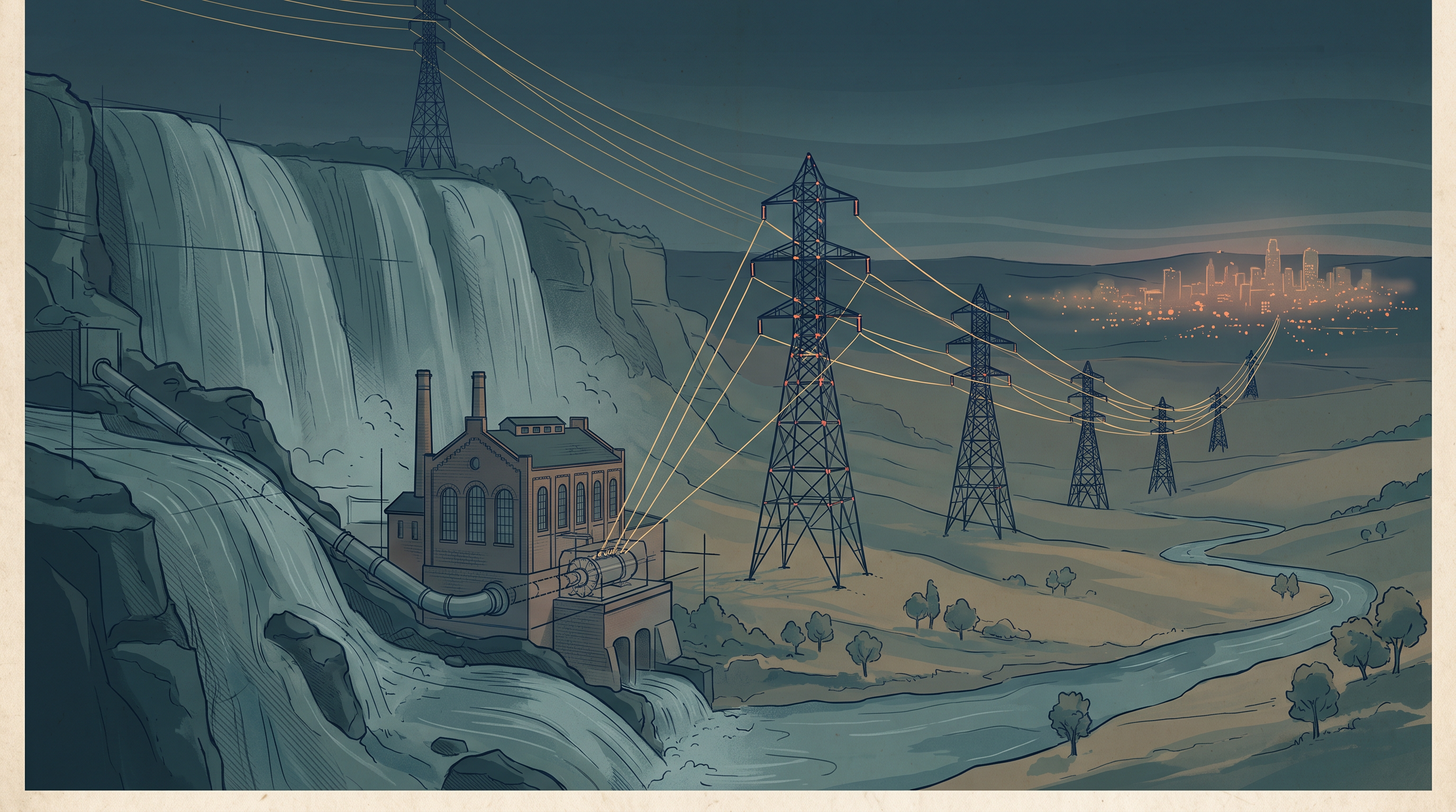
Fig. 7.0 – Niagara Falls and the triumph of alternating current.
As you work through this chapter, you will find the answer to each of these questions.
7.1 Introduction
Until now, we have studied direct current (dc) sources and the circuits they drive. In a dc circuit, the current always flows in the same direction and does not reverse with time. The steady current supplied by a battery is a familiar example of direct current.
But not every current behaves this way. Currents and voltages that change with time are extremely common. In fact, the electricity supplied to our homes, schools, and offices does not stay steady at all. Its value rises and falls, and even reverses direction, following a smooth sine-wave pattern in time.
Before going further, recall what the word voltage means. It is simply the potential difference between two points in a circuit. When this potential difference varies with time like a sine function, we call it an alternating voltage, usually shortened to ac voltage. The current that such a voltage drives through a circuit — a current that also keeps reversing direction — is called alternating current, or ac current.
Most of the electrical devices we use today are designed to run on ac voltage. The main reason is practical. Nearly all the electrical energy sold by power companies is generated, transmitted, and distributed as alternating current, so ac is simply what arrives at our wall sockets.
Why do power companies prefer ac over dc? The chief advantage is that an ac voltage can be raised or lowered easily and efficiently using a device called a transformer. Changing one dc voltage into another is far more difficult. Because ac voltage can be stepped up and down so conveniently, electrical energy can also be transmitted economically over very long distances, with much smaller losses in the wires.
Beyond making transmission easy, ac circuits also show special behaviours that engineers put to clever use in everyday devices. For example, when you tune a radio to pick out your favourite station from all the signals in the air, you are quietly making use of one such property of ac circuits — just one of many that you will meet in this chapter.
7.2 AC Voltage Applied to a Resistor
Let us begin with the simplest ac circuit: a single resistor \(R\) connected across a source of ac voltage. This is shown in Fig. 7.1. In circuit diagrams, an ac source is drawn as a circle with a wavy line inside it (the wavy line stands for the sinusoidal, or sine-shaped, output).
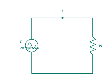
Fig. 7.1 – Purely resistive ac circuit.
We take a source whose potential difference across its terminals varies sinusoidally with time. This ac voltage is written as
\[v = v_m \sin \omega t \tag{7.1}\]
Here \(v\) is the instantaneous voltage at time \(t\) (in volts, V). The symbol \(v_m\) is the amplitude — the maximum, or peak, value that the oscillating voltage reaches (also in volts). The symbol \(\omega\) is the angular frequency of the source, measured in radians per second (rad/s).
It is useful to recall that angular frequency is related to the ordinary frequency \(\nu\) (the number of complete cycles per second, measured in hertz, Hz) by \(\omega = 2\pi\nu\). So the 50 Hz mains supply corresponds to \(\omega = 2\pi \times 50\) rad/s.
Finding the current
To find the current through the resistor, we apply Kirchhoff’s loop rule, \(\sum \varepsilon(t) = 0\) (first met in Section 3.12), to the circuit of Fig. 7.1. This rule states that, at every instant, the sum of the potential changes around a closed loop must be zero. Going around this single loop, the voltage supplied by the source equals the voltage drop across the resistor:
\[v_m \sin \omega t = i R\]
Rearranging,
\[i = \frac{v_m}{R} \sin \omega t\]
Since \(R\) is a constant, this can be written as
\[i = i_m \sin \omega t \tag{7.2}\]
where the current amplitude \(i_m\) (the peak current, in amperes) is
\[i_m = \frac{v_m}{R} \tag{7.3}\]
Equation (7.3) is simply Ohm’s law. Notice that for a resistor it works equally well whether the voltage is ac or dc.
Voltage and current are in phase
Both the applied voltage (Eq. 7.1) and the resulting current (Eq. 7.2) are sine functions of time. When we plot them together against time, as in Fig. 7.2, we see that they rise, fall, and cross zero at exactly the same instants — both reach their maximum together, both reach their minimum together, and both are zero together.
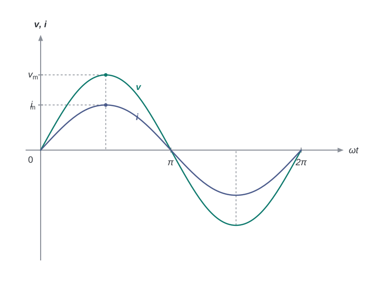
Fig. 7.2 – Voltage and current in a pure resistor.
Because their peaks and zeros line up perfectly, we say the voltage and current are in phase. The phase angle between them is zero.
Average current is zero, but power is not
Like the applied voltage, the current varies sinusoidally, taking positive values during one half of each cycle and equal negative values during the other half. Added up over one complete cycle, these positive and negative values cancel, so the average current over a full cycle is zero.
This might suggest that no energy is delivered — but that is not the case. The heat produced in a resistor (called Joule heating) is given by \(i^2 R\), and it depends on \(i^2\), not on \(i\). Since \(i^2\) is always positive (squaring a negative number gives a positive number), heat is produced during both halves of the cycle. So an alternating current does dissipate electrical energy and does heat a resistor, even though its average value is zero.
Average power in a resistor
The instantaneous power dissipated in the resistor is
\[p = i^2 R = i_m^2 R \sin^2 \omega t \tag{7.4}\]
To find the average power over one cycle, we take the average of this expression. We write the average value of a quantity using a bar over the symbol, or angle brackets \(\langle \; \rangle\) around it:
\[\bar{p} = \langle i^2 R \rangle = \langle i_m^2 R \sin^2 \omega t \rangle \tag{7.5a}\]
The average value of any function \(F(t)\) over a period \(T\) is found from \(\langle F(t) \rangle = \dfrac{1}{T}\displaystyle\int_0^T F(t)\, dt\) — that is, we add up the function over one full cycle and divide by the length of the cycle.
Since \(i_m^2\) and \(R\) are constants, they come out of the average:
\[\bar{p} = i_m^2 R \, \langle \sin^2 \omega t \rangle \tag{7.5b}\]
Now we use the trigonometric identity \(\sin^2 \omega t = \tfrac{1}{2}(1 - \cos 2\omega t)\). Taking averages of both sides,
\[\langle \sin^2 \omega t \rangle = \tfrac{1}{2}\left(1 - \langle \cos 2\omega t \rangle\right)\]
The average of \(\cos 2\omega t\) over a full cycle is zero, because the cosine spends equal time positive and negative, so these contributions cancel. Therefore
\[\langle \sin^2 \omega t \rangle = \frac{1}{2}\]
Substituting this back, the average power is
\[\bar{p} = \frac{1}{2} i_m^2 R \tag{7.5c}\]
The rms (effective) current and voltage
For direct current, we write power simply as \(P = I^2 R\). To put ac power in the same neat form, we define a special value of current called the root mean square (rms) current, also called the effective current. It is written as \(I_{rms}\) or just \(I\), and is shown in relation to the peak current in Fig. 7.3.
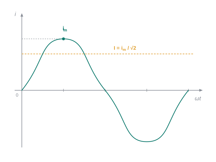
Fig. 7.3 – Peak and rms values of an alternating current.
The name describes exactly how it is calculated: take the square of the current, find its mean (average) over a cycle, and then take the square root. This gives
\[I = \sqrt{\overline{i^2}} = \sqrt{\frac{1}{2} i_m^2} = \frac{i_m}{\sqrt{2}} = 0.707\, i_m \tag{7.6}\]
In terms of \(I\), the average power becomes
\[P = \bar{p} = \frac{1}{2} i_m^2 R = I^2 R \tag{7.7}\]
which has exactly the same form as the dc power expression. In the same way, we define the rms voltage (or effective voltage):
\[V = \frac{v_m}{\sqrt{2}} = 0.707\, v_m \tag{7.8}\]
Now, from Eq. (7.3) we had \(v_m = i_m R\). Dividing both sides by \(\sqrt{2}\),
\[\frac{v_m}{\sqrt{2}} = \frac{i_m}{\sqrt{2}} R\]
which gives, using the rms definitions,
\[V = I R \tag{7.9}\]
Equation (7.9) links ac voltage and ac current, and it has the same simple form as Ohm’s law in the dc case. This is the great advantage of using rms values: with them, the power equation (7.7) and the voltage–current relation (7.9) for ac circuits look exactly like the familiar dc equations.
Why rms values are quoted in practice
It is standard to measure and quote rms values for ac quantities. For instance, the household line voltage of 220 V is an rms value; its peak value is
\[v_m = \sqrt{2}\, V = (1.414)(220\ \text{V}) = 311\ \text{V}\]
In fact, the rms current \(I\) is the equivalent dc current — the steady dc current that would produce exactly the same average heating in the resistor as the alternating current does. This is precisely why rms is the natural, physically meaningful value to report.
Finally, Eq. (7.7) can also be written in two other familiar forms:
\[P = \frac{V^2}{R} = I V \qquad (\text{since } V = I R)\]
7.3 Representation of AC Current and Voltage by Rotating Vectors — Phasors
In the previous section we saw that, for a pure resistor, the current is in phase with the applied ac voltage — their peaks and zeros line up exactly. But this simple picture does not hold for every circuit element. When the circuit contains an inductor, a capacitor, or a mixture of these, the current is no longer in step with the voltage; one may lead or lag the other.
To keep track of these phase relationships neatly, we use a tool called a phasor, and the picture we draw with them is called a phasor diagram. Phasors make analysing ac circuits much easier, because they turn the problem of adding sine waves into the familiar problem of adding vectors.
A phasor is an arrow (a vector) that rotates about the origin with angular speed \(\omega\), as shown in Fig. 7.4(a). Its length represents the amplitude (peak value) of an oscillating quantity, and its rotation represents how that quantity varies in time.
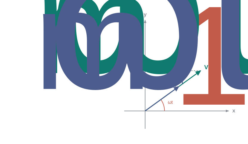
Fig. 7.4(a) – Phasor diagram for a resistive circuit.
Let us see how a phasor stands for a sine wave. In the diagram, the voltage phasor \(\mathbf{V}\) has length equal to the peak voltage \(v_m\), and the current phasor \(\mathbf{I}\) has length equal to the peak current \(i_m\). As the source runs, each phasor rotates steadily, so after a time \(t\) it has turned through an angle \(\omega t\). The vertical component (projection) of the voltage phasor is then \(v_m \sin \omega t\), and that of the current phasor is \(i_m \sin \omega t\). These projections are exactly the instantaneous values \(v\) and \(i\) at that moment.
Figure 7.4(a) shows the two phasors at a particular instant \(t_1\), for the resistor circuit of Fig. 7.1. As the phasors keep rotating with angular frequency \(\omega\), their vertical projections rise and fall, tracing out the sine curves of voltage and current shown in Fig. 7.5(b).
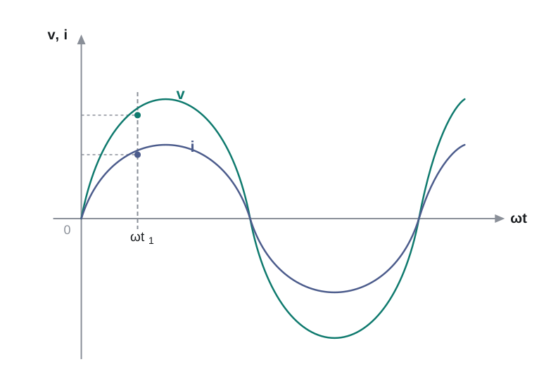
Fig. 7.5(b) – Voltage and current graphs corresponding to the phasors.
Notice in Fig. 7.4(a) that, for a resistor, the voltage phasor \(\mathbf{V}\) and the current phasor \(\mathbf{I}\) point in the same direction. This remains true at every instant as they rotate together. In other words, the angle between them stays zero — which is just the phasor way of saying that the phase angle between voltage and current is zero, and the two are in phase.
7.4 AC Voltage Applied to an Inductor
We now connect an ac source to an inductor instead of a resistor, as shown in Fig. 7.6. In real life, the coil of wire that makes up an inductor always has some resistance in its windings. To study the inductor’s effect on its own, we assume this resistance is negligibly small. The circuit is then a purely inductive ac circuit.
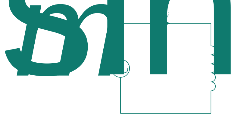
Fig. 7.6 – Purely inductive ac circuit.
Let the source voltage be \(v = v_m \sin \omega t\). Applying Kirchhoff’s loop rule, \(\sum \varepsilon(t) = 0\), and remembering that there is no resistor in the circuit, we get
\[v - L\frac{di}{dt} = 0 \tag{7.10}\]
The second term here is the self-induced emf in the inductor. Recall from Chapter 6 that when the current through a coil changes, the changing magnetic flux linked with the coil induces an emf in the coil itself, equal to \(-L\,di/dt\). The quantity \(L\) is the self-inductance of the coil, measured in henry (H). The negative sign is a consequence of Lenz’s law: the induced emf always opposes the change in current that produces it.
Finding the current
Rearranging Eq. (7.10) and using \(v = v_m \sin \omega t\) (Eq. 7.1),
\[\frac{di}{dt} = \frac{v}{L} = \frac{v_m}{L}\sin \omega t \tag{7.11}\]
Equation (7.11) tells us that the current \(i(t)\) must be a function whose slope, \(di/dt\), is itself a sine function — in phase with the source voltage and with amplitude \(v_m/L\). To recover the current from its rate of change, we integrate both sides with respect to time:
\[\int \frac{di}{dt}\, dt = \frac{v_m}{L}\int \sin(\omega t)\, dt\]
Carrying out the integration (recall that \(\int \sin \omega t\, dt = -\dfrac{\cos \omega t}{\omega}\)),
\[i = -\frac{v_m}{\omega L}\cos(\omega t) + \text{constant}\]
The constant of integration has the units of current and does not change with time. But the source emf swings symmetrically above and below zero, so the current it drives must also swing symmetrically about zero — it can have no steady, time-independent part. Therefore this integration constant must be zero.
To write the current in the standard sine form, we use the trigonometric identity \(-\cos(\omega t) = \sin\!\left(\omega t - \dfrac{\pi}{2}\right)\). This gives
\[i = i_m \sin\!\left(\omega t - \frac{\pi}{2}\right) \tag{7.12}\]
where the current amplitude is \(i_m = \dfrac{v_m}{\omega L}\).
Inductive reactance
The quantity \(\omega L\) plays the same role for an inductor that resistance plays for a resistor — it opposes and limits the current. We call it the inductive reactance, written \(X_L\):
\[X_L = \omega L \tag{7.13}\]
so that the current amplitude can be written neatly as
\[i_m = \frac{v_m}{X_L} \tag{7.14}\]
Inductive reactance has the same dimensions and SI unit (ohm, \(\Omega\)) as resistance, and it limits current in a purely inductive circuit just as resistance does in a purely resistive one. Notice from \(X_L = \omega L\) that the inductive reactance grows in direct proportion both to the inductance \(L\) and to the frequency of the source. A higher-frequency supply, or a larger inductor, means a greater opposition to the current.
The current lags the voltage
Compare the source voltage, \(v = v_m \sin \omega t\) (Eq. 7.1), with the current, \(i = i_m \sin(\omega t - \pi/2)\) (Eq. 7.12). The current is the same sine shape but shifted back by \(\pi/2\). This means the current lags the voltage by \(\pi/2\), that is, by one-quarter of a full cycle.
Figure 7.7(a) shows the voltage and current phasors at an instant \(t_1\). The current phasor \(\mathbf{I}\) sits \(\pi/2\) behind the voltage phasor \(\mathbf{V}\). As both rotate counter-clockwise at frequency \(\omega\), their vertical projections generate the voltage and current curves of Fig. 7.8(b).
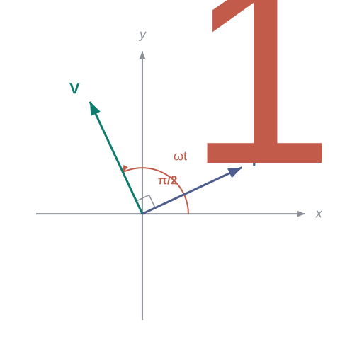
Fig. 7.7(a) – Phasor diagram for an inductive circuit.
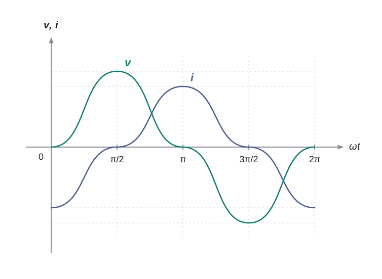
Fig. 7.8(b) – Voltage and current in a pure inductor.
In graphical terms (Fig. 7.8b), the current reaches its maximum a quarter of a period after the voltage does, the delay being \(\dfrac{T}{4} = \dfrac{\pi/2}{\omega}\).
Does an inductor consume power?
An inductor limits current like a resistance does, so it is natural to ask whether it also dissipates energy the way a resistor does. Let us check by finding the average power.
The instantaneous power delivered to the inductor is the product of the instantaneous current and voltage:
\[p_L = i\,v = i_m \sin\!\left(\omega t - \frac{\pi}{2}\right) \times v_m \sin(\omega t)\]
Since \(\sin(\omega t - \pi/2) = -\cos \omega t\), this becomes
\[p_L = -i_m v_m \cos(\omega t)\sin(\omega t) = -\frac{i_m v_m}{2}\sin(2\omega t)\]
The average power over one complete cycle is then
\[P_L = \left\langle -\frac{i_m v_m}{2}\sin(2\omega t)\right\rangle = -\frac{i_m v_m}{2}\big\langle \sin(2\omega t)\big\rangle = 0\]
because the average of \(\sin(2\omega t)\) over a full cycle is zero (it spends equal time positive and negative). So, over one complete cycle, the net power supplied to a pure inductor is zero.
7.5 AC Voltage Applied to a Capacitor
Next we connect an ac source, generating \(v = v_m \sin \omega t\), across a capacitor alone, as shown in Fig. 7.9. This is a purely capacitive ac circuit.

Fig. 7.9 – Purely capacitive ac circuit.
To see what a capacitor does with ac, first recall its behaviour with dc. When a capacitor is joined to a dc source, current flows only for the brief time needed to charge it. As charge piles up on the plates, the voltage across the capacitor rises and pushes back against the incoming current. Once the capacitor is fully charged, this opposing voltage matches the source and the current drops to zero. So in a dc circuit a capacitor eventually blocks the current completely.
An ac source behaves very differently. Because the source voltage keeps reversing, the capacitor is alternately charged and discharged during each half cycle: charge flows onto the plates, then off again, then on with opposite polarity, and so on. The current in the connecting wires never gets a chance to settle to zero — it keeps flowing back and forth. The capacitor still limits the current, but it no longer stops it.
This is why a lamp placed in series with a capacitor stays dark on a dc supply (once the capacitor charges, current stops) but glows on an ac supply (the alternating charging and discharging keeps current flowing).
Finding the current
Let \(q\) be the charge on the capacitor at time \(t\). The instantaneous voltage across a capacitor of capacitance \(C\) is
\[v = \frac{q}{C} \tag{7.15}\]
By Kirchhoff’s loop rule, the source voltage equals the capacitor voltage at every instant:
\[v_m \sin \omega t = \frac{q}{C}\]
so the charge on the plates is \(q = C v_m \sin \omega t\). The current is the rate at which this charge changes, \(i = \dfrac{dq}{dt}\):
\[i = \frac{d}{dt}\big(C v_m \sin \omega t\big) = \omega C v_m \cos(\omega t)\]
Using the identity \(\cos(\omega t) = \sin\!\left(\omega t + \dfrac{\pi}{2}\right)\), we can write this in the standard sine form:
\[i = i_m \sin\!\left(\omega t + \frac{\pi}{2}\right) \tag{7.16}\]
where the current amplitude is \(i_m = \omega C v_m\). Rewriting this,
\[i_m = \frac{v_m}{(1/\omega C)}\]
Capacitive reactance
Comparing \(i_m = v_m/(1/\omega C)\) with \(i_m = v_m/R\) for a resistor, we see that the quantity \(\left(1/\omega C\right)\) plays the part of resistance here. It is called the capacitive reactance, written \(X_C\):
\[X_C = \frac{1}{\omega C} \tag{7.17}\]
so that the current amplitude becomes
\[i_m = \frac{v_m}{X_C} \tag{7.18}\]
Capacitive reactance has the same dimensions and SI unit (ohm, \(\Omega\)) as resistance, and it limits the current amplitude in a purely capacitive circuit just as resistance does in a resistive one. But notice the crucial difference from inductive reactance: because \(X_C = 1/\omega C\), the capacitive reactance is inversely proportional to both the frequency and the capacitance. Raising the frequency (or using a larger capacitor) makes \(X_C\) smaller and lets more current through — the opposite of what an inductor does.
The current leads the voltage
Compare the current, \(i = i_m \sin(\omega t + \pi/2)\) (Eq. 7.16), with the source voltage, \(v = v_m \sin \omega t\) (Eq. 7.1). The current is shifted forward by \(\pi/2\), so the current leads the voltage by \(\pi/2\) — one-quarter of a cycle. This is exactly the reverse of the inductor, where the current lagged by \(\pi/2\).
Figure 7.10(a) shows the phasor diagram at an instant \(t_1\): the current phasor \(\mathbf{I}\) is a quarter turn ahead of the voltage phasor \(\mathbf{V}\) as they rotate counter-clockwise. Figure 7.11(b) shows the corresponding time graphs, in which the current reaches its peak a quarter period earlier than the voltage.
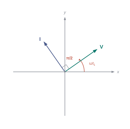
Fig. 7.10(a) – Phasor diagram for a capacitive circuit.
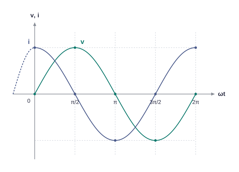
Fig. 7.11(b) – Voltage and current in a pure capacitor.
Power in a capacitor
As with the inductor, we check whether the capacitor consumes energy. The instantaneous power supplied is
\[p_C = i\,v = i_m \cos(\omega t)\, v_m \sin(\omega t) = i_m v_m \cos(\omega t)\sin(\omega t) = \frac{i_m v_m}{2}\sin(2\omega t) \tag{7.19}\]
Averaging over one complete cycle,
\[P_C = \left\langle \frac{i_m v_m}{2}\sin(2\omega t)\right\rangle = \frac{i_m v_m}{2}\big\langle \sin(2\omega t)\big\rangle = 0\]
since the average of \(\sin(2\omega t)\) over a full cycle is zero. So a pure capacitor, like a pure inductor, uses no net power.
A light bulb and an open coil inductor are connected to an ac source through a key, as shown in Fig. 7.12. The switch is closed, and after some time an iron rod is inserted into the interior of the inductor. Does the glow of the bulb (a) increase, (b) decrease, or (c) stay unchanged as the rod is inserted? Give reasons.
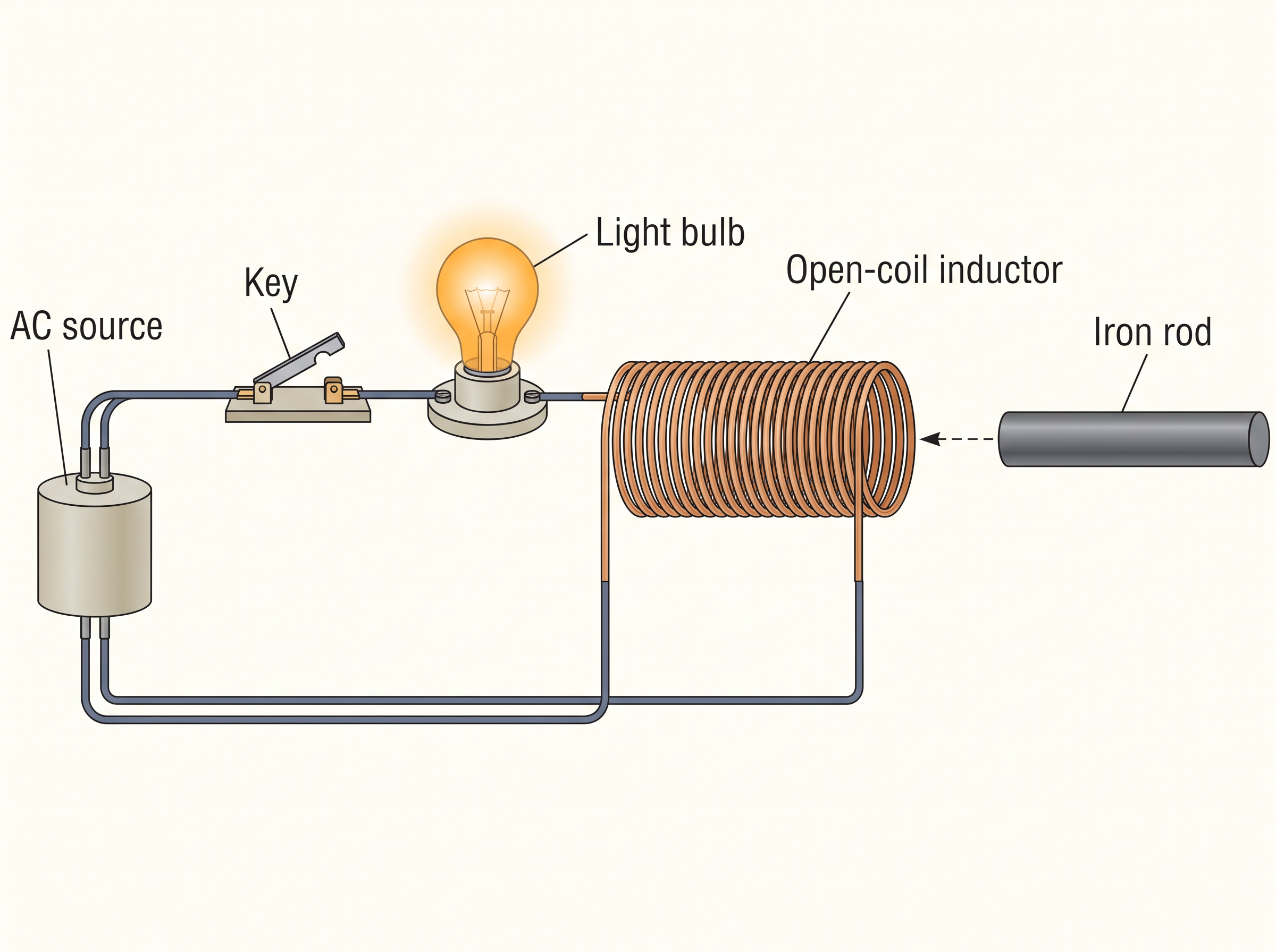
[Caption:] Fig. 7.12 – Inserting an iron core into an inductor. [/Caption:]
Solution As the iron rod is pushed in, the magnetic field of the coil magnetises the iron, which greatly increases the magnetic field inside the coil. This raises the inductance \(L\) of the coil, and therefore its inductive reactance \(X_L = \omega L\) rises as well. With larger reactance, a bigger share of the applied ac voltage appears across the inductor, leaving less voltage for the bulb. So less current flows through the bulb, and its glow decreases.
7.6 AC Voltage Applied to a Series LCR Circuit
We now bring all three elements together: a resistor \(R\), an inductor \(L\), and a capacitor \(C\) joined one after another (in series) across an ac source, as shown in Fig. 7.13. As before, the source voltage is \(v = v_m \sin \omega t\).
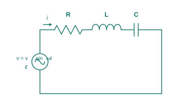
Fig. 7.13 – Series LCR circuit.
Let \(q\) be the charge on the capacitor and \(i\) the current at time \(t\). Applying Kirchhoff’s loop rule around this single loop, the source voltage equals the sum of the voltage drops across the three elements:
\[L\frac{di}{dt} + iR + \frac{q}{C} = v \tag{7.20}\]
Our goal is to find the instantaneous current \(i\) and how its phase compares with the applied voltage \(v\). This can be done in two ways. The first uses the phasor technique we have been building up; the second solves Eq. (7.20) analytically to get the time-dependence of \(i\) directly. We follow the phasor method here.
7.6.1 Phasor-diagram solution
Because \(R\), \(L\), and \(C\) are in series (Fig. 7.13), the same current flows through each of them at every instant — same amplitude, same phase. Let this common current be
\[i = i_m \sin(\omega t + \phi) \tag{7.21}\]
Here \(\phi\) is the phase difference between the source voltage and the current. We do not yet know its value or sign; the phasor diagram will give it to us.
Let \(\mathbf{I}\) be the phasor for the current in Eq. (7.21). Let \(\mathbf{V_L}\), \(\mathbf{V_R}\), \(\mathbf{V_C}\), and \(\mathbf{V}\) be the phasors for the voltages across the inductor, resistor, capacitor, and source, respectively. From the earlier sections we already know the phase relationships each element has with the current:
- \(\mathbf{V_R}\) is parallel to \(\mathbf{I}\) (resistor voltage is in phase with the current),
- \(\mathbf{V_C}\) is \(\pi/2\) behind \(\mathbf{I}\) (capacitor voltage lags the current — equivalently, current leads),
- \(\mathbf{V_L}\) is \(\pi/2\) ahead of \(\mathbf{I}\) (inductor voltage leads the current — equivalently, current lags).
These four phasors are drawn with their correct phase relations in Fig. 7.14(a).
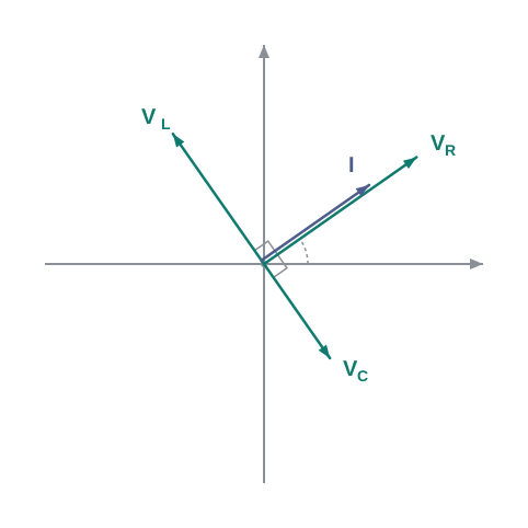
Fig. 7.14(a) – Phase relationship of voltages in an LCR circuit.
The lengths of these voltage phasors are their amplitudes:
\[v_{Rm} = i_m R, \qquad v_{Cm} = i_m X_C, \qquad v_{Lm} = i_m X_L \tag{7.22}\]
The loop equation (7.20) in terms of the instantaneous voltages is simply
\[v_L + v_R + v_C = v \tag{7.23}\]
The phasor equation whose vertical components reproduce Eq. (7.23) is the vector sum
\[\mathbf{V_L} + \mathbf{V_R} + \mathbf{V_C} = \mathbf{V} \tag{7.24}\]
This addition is shown in Fig. 7.15(b).
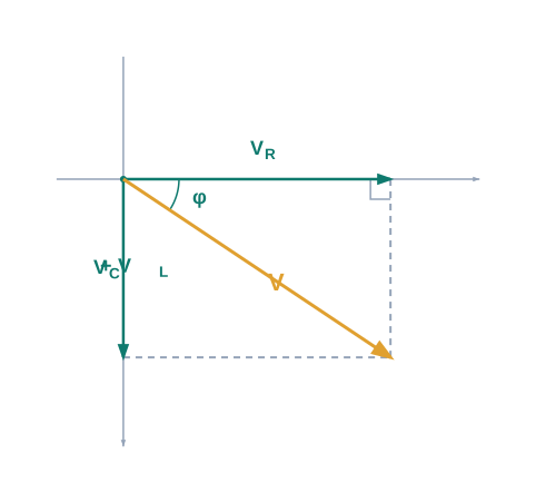
Fig. 7.15(b) – Vector addition of voltage phasors.
Now, \(\mathbf{V_L}\) and \(\mathbf{V_C}\) always lie along the same straight line but point in opposite directions (one leads the current by \(\pi/2\), the other lags by \(\pi/2\)). So they partly cancel, and can be combined into a single phasor \((\mathbf{V_C} + \mathbf{V_L})\) whose magnitude is the difference \(\left| v_{Cm} - v_{Lm}\right|\).
The source phasor \(\mathbf{V}\) is the hypotenuse of a right-angled triangle whose two perpendicular sides are \(\mathbf{V_R}\) and \((\mathbf{V_C} + \mathbf{V_L})\). By the Pythagorean theorem,
\[v_m^2 = v_{Rm}^2 + \left(v_{Cm} - v_{Lm}\right)^2\]
Substituting the amplitudes from Eq. (7.22),
\[v_m^2 = (i_m R)^2 + (i_m X_C - i_m X_L)^2 = i_m^2\left[R^2 + (X_C - X_L)^2\right]\]
Solving for the current amplitude,
\[i_m = \frac{v_m}{\sqrt{R^2 + (X_C - X_L)^2}} \tag{7.25a}\]
Impedance
By analogy with resistance, we define a single quantity called the impedance \(Z\) that captures the total opposition of the whole LCR circuit:
\[i_m = \frac{v_m}{Z} \tag{7.25b}\]
where
\[Z = \sqrt{R^2 + (X_C - X_L)^2} \tag{7.26}\]
The phase angle
Since \(\mathbf{I}\) is always parallel to \(\mathbf{V_R}\), the phase angle \(\phi\) between the source voltage and the current is the angle between \(\mathbf{V_R}\) and \(\mathbf{V}\). From the right triangle in Fig. 7.16,
\[\tan\phi = \frac{v_{Cm} - v_{Lm}}{v_{Rm}}\]
and using the amplitudes from Eq. (7.22),
\[\tan\phi = \frac{X_C - X_L}{R} \tag{7.27}\]
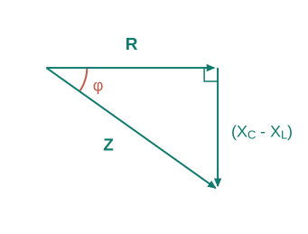
Fig. 7.16 – Impedance diagram for a series LCR circuit.
Equations (7.26) and (7.27) are drawn together in Fig. 7.16 as the impedance diagram — a right triangle with \(Z\) as its hypotenuse, \(R\) along the base, and \((X_C - X_L)\) as the vertical side.
Together, Eq. (7.25a) gives the amplitude of the current and Eq. (7.27) gives its phase angle. With both known, the current in Eq. (7.21) is completely determined.
The sign of \(\phi\) tells us the character of the circuit:
- If \(X_C > X_L\), then \(\phi\) is positive: the circuit is predominantly capacitive, and the current leads the source voltage.
- If \(X_C < X_L\), then \(\phi\) is negative: the circuit is predominantly inductive, and the current lags the source voltage.
Figure 7.17 shows the phasor diagram and the time graphs of \(v\) and \(i\) for the case \(X_C > X_L\).
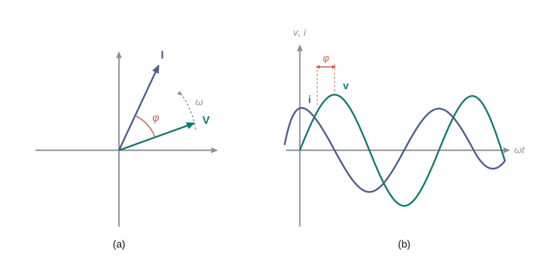
Fig. 7.17(a) – Phasor diagram and (b) time graphs for X_C > X_L.
Steady-state and transient behaviour
This phasor approach gives us the amplitude and phase of the current, but it has a limitation: the phasor diagram says nothing about the initial conditions. We may pick any instant \(t\) (such as \(t_1\), as done throughout this chapter) and draw the phasors showing only their relative angles. The solution obtained this way is the steady-state solution — it is not the complete, general solution.
In fact there is also a transient solution, which is present even when \(v = 0\). The full general solution is the sum of the transient and the steady-state parts. However, after a sufficiently long time the transient part dies away, and the circuit’s behaviour is described entirely by the steady-state solution. This is why the steady-state result is the one that matters in practice.
7.6.2 Resonance
A striking feature of the series LCR circuit is resonance. Resonance is common to any system that naturally tends to oscillate at a particular frequency, called its natural frequency. When such a system is driven by an outside source whose frequency is close to the natural frequency, the oscillations grow large.
A child on a swing is a familiar example. The swing has its own natural frequency for moving back and forth, like a pendulum. If the child (or a pushing parent) pulls on the ropes at regular intervals, and the frequency of these pushes nearly matches the swing’s natural frequency, the swinging builds up to a large amplitude. Small, well-timed pushes add up.
For an LCR circuit driven at frequency \(\omega\) with voltage amplitude \(v_m\), we found the current amplitude to be
\[i_m = \frac{v_m}{Z} = \frac{v_m}{\sqrt{R^2 + (X_C - X_L)^2}}\]
with \(X_C = 1/\omega C\) and \(X_L = \omega L\). Both reactances depend on \(\omega\). So as we vary \(\omega\), there is one special frequency \(\omega_0\) at which the two reactances become equal, \(X_C = X_L\). At that frequency the term \((X_C - X_L)\) vanishes, and the impedance drops to its smallest possible value:
\[Z = \sqrt{R^2 + 0^2} = R\]
This frequency is called the resonant frequency. Setting \(X_C = X_L\):
\[\frac{1}{\omega_0 C} = \omega_0 L\]
which gives
\[\omega_0 = \frac{1}{\sqrt{LC}} \tag{7.28}\]
Since \(Z = R\) at resonance, the current amplitude there is at its maximum, \(i_m = v_m/R\).
Figure 7.18 shows how \(i_m\) varies with \(\omega\) for a series LCR circuit with \(L = 1.00\) mH and \(C = 1.00\) nF, for two resistances: (i) \(R = 100\ \Omega\) and (ii) \(R = 200\ \Omega\), with an applied \(v_m = 100\) V. The resonant frequency for these values is
\[\omega_0 = \frac{1}{\sqrt{LC}} = 1.00\times 10^{6}\ \text{rad/s}\]
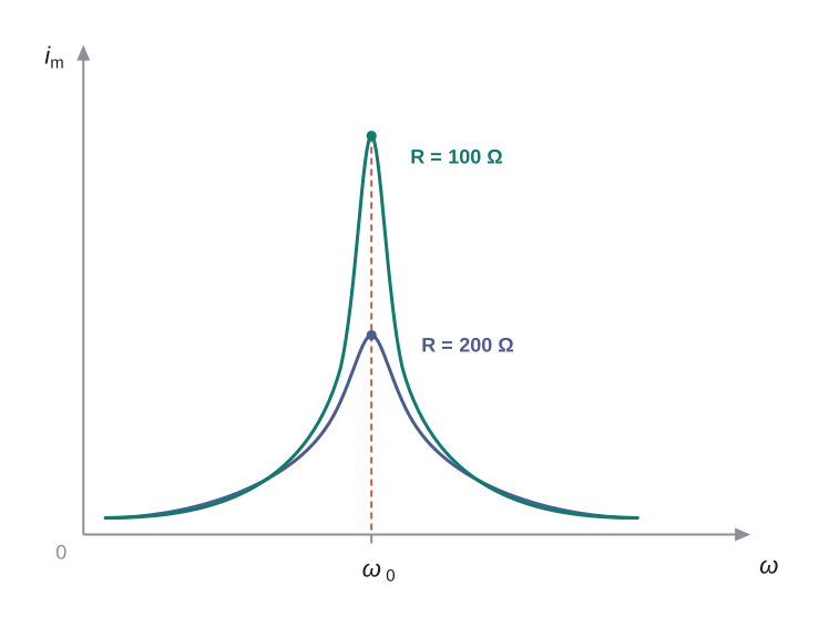
Fig. 7.18 – Resonance curves for two different resistance values.
The current amplitude peaks at \(\omega_0\) in both cases. Because \(i_m = v_m/R\) at resonance, the peak for case (i) is exactly twice that for case (ii) — the smaller the resistance, the taller and sharper the resonance peak.
Resonant circuits are put to work in many devices, most famously in the tuning mechanism of a radio or television. A radio antenna picks up signals from many broadcasting stations at once. These signals act as sources feeding the tuning circuit, so the circuit is being driven at many frequencies together. To listen to just one station, we tune the radio: we vary a capacitor in the tuning circuit until the circuit’s resonant frequency matches the frequency of the desired station’s signal. At that setting, the current due to that one station’s frequency becomes maximum, while all the others produce only small currents — so that station stands out clearly.
One more important point: resonance can occur only if both \(L\) and \(C\) are present. Only then can the inductor and capacitor voltages (which are out of phase) cancel each other, leaving the impedance equal to \(R\) and the full source voltage across the resistor, with \(i_m = v_m/R\). A circuit containing only \(R\) and \(L\), or only \(R\) and \(C\), has no such cancellation and therefore cannot resonate.
7.7 Power in AC Circuit: The Power Factor
We have seen that a voltage \(v = v_m \sin\omega t\) applied to a series LCR circuit drives a current
\[i = i_m \sin(\omega t + \phi), \qquad \text{where} \quad i_m = \frac{v_m}{Z} \quad \text{and} \quad \phi = \tan^{-1}\!\left(\frac{X_C - X_L}{R}\right)\]
Now we ask: how much power does the source actually deliver on average?
Instantaneous and average power
The instantaneous power supplied by the source is the product of the instantaneous voltage and current:
\[p = v\,i = \big(v_m \sin\omega t\big)\times\big[i_m \sin(\omega t + \phi)\big]\]
To simplify the product of two sines, we use the identity \(\sin A \sin B = \tfrac{1}{2}\big[\cos(A - B) - \cos(A + B)\big]\). With \(A = \omega t\) and \(B = \omega t + \phi\), this gives
\[p = \frac{v_m i_m}{2}\big[\cos\phi - \cos(2\omega t + \phi)\big] \tag{7.29}\]
The right-hand side has two parts. The first, \(\cos\phi\), is a constant. The second, \(\cos(2\omega t + \phi)\), oscillates in time — and its average over a full cycle is zero, because its positive and negative halves cancel. So when we average over a cycle, only the constant part survives:
\[P = \frac{v_m i_m}{2}\cos\phi = \frac{v_m}{\sqrt{2}}\cdot\frac{i_m}{\sqrt{2}}\cos\phi = V I \cos\phi \tag{7.30a}\]
where \(V\) and \(I\) are the rms voltage and rms current. Since \(V = IZ\), this can also be written as
\[P = I^2 Z \cos\phi \tag{7.30b}\]
The power factor
The average power therefore depends on the cosine of the phase angle \(\phi\) between voltage and current. This quantity \(\cos\phi\) is called the power factor.
Let us look at four important cases.
Case (i) — Resistive circuit. If the circuit contains only a pure resistor, then \(\phi = 0\) and \(\cos\phi = 1\). Here the power dissipation is maximum for a given voltage and current.
Case (ii) — Purely inductive or purely capacitive circuit. If the circuit is just an inductor or just a capacitor, the phase difference between voltage and current is \(\pi/2\). Then \(\cos\phi = 0\), and no power is dissipated even though a current flows. Such a current is called a wattless current.
Case (iii) — LCR series circuit. In a general series LCR circuit, the power is given by Eq. (7.30), with \(\phi = \tan^{-1}\big[(X_C - X_L)/R\big]\). The phase angle may be non-zero in an RL, RC, or RLC circuit. In every such case, whatever power is dissipated is dissipated only in the resistor — the inductor and capacitor consume none on average.
Case (iv) — At resonance. At the resonant frequency, \(X_C - X_L = 0\), so \(\phi = 0\) and \(\cos\phi = 1\). Then \(P = I^2 Z = I^2 R\), and the power dissipated is maximum. That is, a series LCR circuit dissipates the most power (through \(R\)) exactly at resonance.
(a) For circuits used to transport electric power, explain why a low power factor means large power loss in transmission. (b) Explain how the power factor can often be improved by connecting a capacitor of suitable value.
Solution
The delivered power is \(P = I V \cos\phi\), where \(\cos\phi\) is the power factor. To supply a fixed power \(P\) at a fixed voltage \(V\), if \(\cos\phi\) is small then the current \(I\) must be made correspondingly large. But a large current causes large heating loss (\(I^2 R\)) in the transmission wires. So a low power factor wastes energy in the lines.
Suppose the current \(I\) lags the voltage by an angle \(\phi\); then the power factor is \(\cos\phi = R/Z\). We can push the power factor towards 1 by making \(Z\) tend towards \(R\). To see how, resolve the current phasor \(\mathbf{I}\) into two parts using the phasor diagram of Fig. 7.19: a component \(I_p\) along the applied voltage \(\mathbf{V}\), and a component \(I_q\) perpendicular to it.
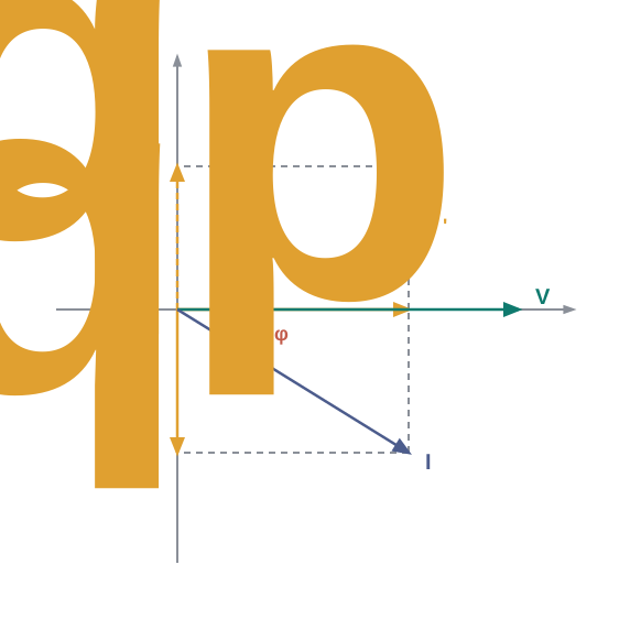
[Caption:] Fig. 7.19 – Resolving current into power and wattless components. [/Caption:]
The perpendicular part \(I_q\) is the wattless component — it carries no power. The in-phase part \(I_p\) is the power component, since it is in phase with the voltage and corresponds to the real power delivered. To improve the power factor, we must cancel the lagging wattless current \(I_q\) with an equal leading wattless current \(I_q'\). This is done by connecting a capacitor of appropriate value in parallel, so that \(I_q\) and \(I_q'\) cancel, leaving the effective power as \(I_p V\).
7.8 Transformers
Very often we need to change (transform) an alternating voltage into a larger or smaller value — for example, to raise the voltage for long-distance transmission, or to lower it for safe use in the home. The device that does this is called a transformer, and it works on the principle of mutual induction.
Recall from Chapter 6 that mutual induction is the effect by which a changing current in one coil induces an emf in a neighbouring coil, through the changing magnetic flux they share. A transformer is built to exploit exactly this effect.
Construction
A transformer has two coils of wire, insulated from each other, wound on a common soft-iron core. The two coils may be wound one on top of the other, as in Fig. 7.20(a), or on separate limbs of the core, as in Fig. 7.20(b). One coil, the primary, has \(N_p\) turns; the other, the secondary, has \(N_s\) turns. Usually the primary is the input coil and the secondary is the output coil.
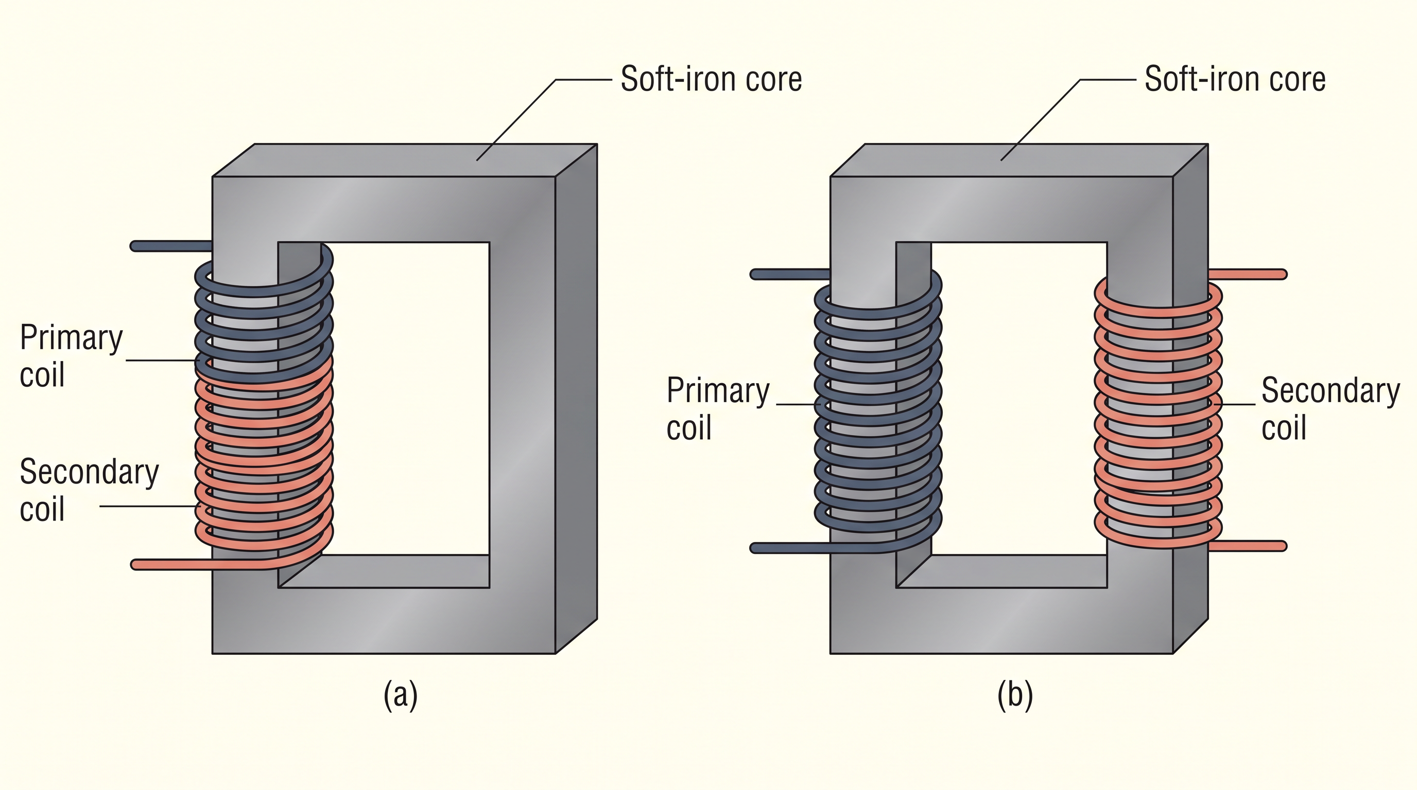
Fig. 7.20(a) – Transformer windings: (a) on the same limb and (b) on separate limbs.
How it works
When an alternating voltage is applied to the primary, the alternating current it drives sets up an alternating magnetic flux in the iron core. Because the core guides this flux through the secondary coil, the changing flux induces an emf in the secondary. The size of that emf depends on how many turns the secondary has.
To keep the analysis clean, we consider an ideal transformer: the primary has negligible resistance, and all the flux in the core links both coils. Let \(\phi\) be the flux through each turn of the core at time \(t\), produced by the primary current when a voltage \(v_p\) is applied.
The emf induced in the secondary (with \(N_s\) turns) is, by Faraday’s law,
\[\varepsilon_s = -N_s \frac{d\phi}{dt} \tag{7.31}\]
The same alternating flux also induces an emf in the primary itself, called the back emf:
\[\varepsilon_p = -N_p \frac{d\phi}{dt} \tag{7.32}\]
Now, \(\varepsilon_p = v_p\). If it were not so, the primary current would be infinite, since we have assumed the primary has zero resistance. And if the secondary is on open circuit (or draws only a small current), then to a good approximation \(\varepsilon_s = v_s\), where \(v_s\) is the secondary voltage. So Eqs. (7.31) and (7.32) become
\[v_s = -N_s \frac{d\phi}{dt} \tag{7.31a}\] \[v_p = -N_p \frac{d\phi}{dt} \tag{7.32a}\]
Dividing one by the other, the common factor \(d\phi/dt\) cancels, leaving the turns relation:
\[\frac{v_s}{v_p} = \frac{N_s}{N_p} \tag{7.33}\]
This result rests on three assumptions: (i) the primary resistance and current are small; (ii) the same flux links both coils, as very little escapes the core; and (iii) the secondary current is small.
Relating currents
If the transformer is taken to be 100% efficient (no energy loss), the power fed in equals the power drawn out. Since power is \(p = iv\),
\[i_p v_p = i_s v_s \tag{7.34}\]
Real transformers always lose a little energy, but this is a good approximation, because a well-designed transformer can be more than 95% efficient. Combining Eqs. (7.33) and (7.34),
\[\frac{i_p}{i_s} = \frac{v_s}{v_p} = \frac{N_s}{N_p} \tag{7.35}\]
Because current and voltage both oscillate at the same frequency as the source, Eq. (7.35) holds equally for the amplitudes or the rms values. We can now write how the transformer changes voltage and current:
\[V_s = \left(\frac{N_s}{N_p}\right)V_p \qquad\text{and}\qquad I_s = \left(\frac{N_p}{N_s}\right)I_p \tag{7.36}\]
Step-up and step-down
If the secondary has more turns than the primary (\(N_s > N_p\)), the voltage is raised: \(V_s > V_p\). This is a step-up transformer. But raising the voltage lowers the current in the secondary (\(I_s < I_p\)). For instance, if the primary has 100 turns and the secondary 200 turns, then \(N_s/N_p = 2\), so a 220 V input at 10 A steps up to a 440 V output at 5.0 A.
If instead the secondary has fewer turns than the primary (\(N_s < N_p\)), the voltage is lowered and the current raised: this is a step-down transformer, with \(V_s < V_p\) and \(I_s > I_p\).
Notice what Eq. (7.36) is telling us: a step-up transformer raises the voltage but lowers the current by exactly the same factor, so the product (the power) stays the same. A transformer does not create energy — it only trades voltage for current, or current for voltage.
Losses in real transformers
The relations above are for an ideal transformer. In a real transformer, small energy losses occur for four main reasons:
- Flux leakage. Not all the flux produced by the primary passes through the secondary, because of imperfect core design or air gaps. This is reduced by winding the two coils one over the other.
- Resistance of the windings. The wire has some resistance, so heat (\(I^2R\)) is lost in it. In high-current, low-voltage windings this is minimised by using thick wire.
- Eddy currents. The alternating flux induces swirling currents in the iron core, which heat it. These are reduced by using a laminated core (thin sheets, instead of a solid block).
- Hysteresis. The core’s magnetisation is reversed again and again by the alternating field, and this repeated reversal costs energy that appears as heat. It is kept small by choosing a magnetic material with low hysteresis loss.
Transformers in power transmission
The large-scale transmission of electrical energy over long distances relies on transformers. At the generating station, the generator’s output voltage is stepped up to a very high value. This reduces the current for the same power, and since transmission-line loss is \(I^2R\), a smaller current means far less energy wasted as heat in the wires. The high-voltage power is then carried over long distances to a sub-station near the consumers, where the voltage is stepped down. It is stepped down further at distributing sub-stations and utility poles, until a supply of about 240 V finally reaches our homes.
7.9 Summary
An alternating voltage \(v = v_m \sin\omega t\) applied to a resistor \(R\) drives a current \(i = i_m \sin\omega t\) through it, with amplitude \(i_m = \dfrac{v_m}{R}\). The current is in phase with the applied voltage.
When an alternating current \(i = i_m \sin\omega t\) passes through a resistor \(R\), the average power dissipated over a cycle (by Joule heating) is \(\tfrac{1}{2} i_m^2 R\). To write this in the same form as the dc power \(P = I^2 R\), we use a special value of current called the root mean square (rms) current \(I\): \[I = \frac{i_m}{\sqrt{2}} = 0.707\, i_m\] Similarly, the rms voltage is \[V = \frac{v_m}{\sqrt{2}} = 0.707\, v_m\] With these, \(P = I V = I^2 R\).
An ac voltage \(v = v_m \sin\omega t\) applied to a pure inductor \(L\) drives a current \(i = i_m \sin\!\left(\omega t - \dfrac{\pi}{2}\right)\), where \(i_m = \dfrac{v_m}{X_L}\). The quantity \(X_L = \omega L\) is the inductive reactance. The current lags the voltage by \(\pi/2\), and the average power supplied to the inductor over a complete cycle is zero.
An ac voltage \(v = v_m \sin\omega t\) applied to a capacitor drives a current \(i = i_m \sin\!\left(\omega t + \dfrac{\pi}{2}\right)\), where \(i_m = \dfrac{v_m}{X_C}\). The quantity \(X_C = \dfrac{1}{\omega C}\) is the capacitive reactance. The current leads the voltage by \(\pi/2\), and (as with the inductor) the average power supplied over a complete cycle is zero.
For a series LCR circuit driven by \(v = v_m \sin\omega t\), the current is \(i = i_m \sin(\omega t + \phi)\), where \[i_m = \frac{v_m}{\sqrt{R^2 + (X_C - X_L)^2}}, \qquad \phi = \tan^{-1}\!\left(\frac{X_C - X_L}{R}\right)\] The quantity \[Z = \sqrt{R^2 + (X_C - X_L)^2}\] is the impedance of the circuit. The average power over a complete cycle is \[P = V I \cos\phi\] and \(\cos\phi\) is called the power factor.
In a purely inductive or purely capacitive circuit, \(\cos\phi = 0\), so no power is dissipated even though a current flows. Such a current is called a wattless current.
The phase relationship between current and voltage in an ac circuit is conveniently shown by representing them as rotating vectors called phasors. A phasor rotates about the origin with angular speed \(\omega\), and its length represents the amplitude (peak value) of the quantity. Phasor diagrams make ac-circuit analysis much easier.
A transformer has a primary coil of \(N_p\) turns and a secondary coil of \(N_s\) turns wound on an iron core. When the primary is connected to an ac source, the voltages are related by \[V_s = \left(\frac{N_s}{N_p}\right)V_p\] and the currents by \[I_s = \left(\frac{N_p}{N_s}\right)I_p\] If the secondary has more turns than the primary, the voltage is stepped up (\(V_s > V_p\)): this is a step-up transformer. If the secondary has fewer turns, it is a step-down transformer.
Key Quantities, Units, and Formulae
| Physical quantity | Symbol | Dimensions | SI Unit | Remarks |
|---|---|---|---|---|
| rms voltage | \(V\) | \([\text{M L}^2\text{T}^{-3}\text{A}^{-1}]\) | V | \(V = \dfrac{v_m}{\sqrt{2}}\); \(v_m\) is the amplitude of the ac voltage |
| rms current | \(I\) | \([\text{A}]\) | A | \(I = \dfrac{i_m}{\sqrt{2}}\); \(i_m\) is the amplitude of the ac current |
| Inductive reactance | \(X_L\) | \([\text{M L}^2\text{T}^{-3}\text{A}^{-2}]\) | \(\Omega\) | \(X_L = \omega L\) |
| Capacitive reactance | \(X_C\) | \([\text{M L}^2\text{T}^{-3}\text{A}^{-2}]\) | \(\Omega\) | \(X_C = \dfrac{1}{\omega C}\) |
| Impedance | \(Z\) | \([\text{M L}^2\text{T}^{-3}\text{A}^{-2}]\) | \(\Omega\) | Depends on the elements present in the circuit |
| Resonant frequency | \(\omega_r\) or \(\omega_0\) | \([\text{T}^{-1}]\) | Hz | \(\omega_0 = \dfrac{1}{\sqrt{LC}}\) for a series RLC circuit |
| Quality factor | \(Q\) | Dimensionless | — | \(Q = \dfrac{\omega_0 L}{R} = \dfrac{1}{\omega_0 C R}\) for a series RLC circuit |
| Power factor | — | Dimensionless | — | \(= \cos\phi\), where \(\phi\) is the phase difference between the applied voltage and the current |
7.10 Points to Ponder
When a value is quoted for an ac voltage or current, it is normally the rms value. The mains outlet in your room is usually rated 240 V — this is the rms voltage, not the peak. Its amplitude (peak value) is \[v_m = \sqrt{2}\,V = \sqrt{2}\,(240) = 340\ \text{V}\]
The power rating marked on an element used in ac circuits refers to its average power rating, not its instantaneous or peak power.
The power consumed in an ac circuit is never negative. (The source may momentarily receive energy back from inductors and capacitors during a cycle, but the average real power delivered is always zero or positive.)
Both ac and dc are measured in amperes — but how is the ampere defined for a current that keeps reversing? The dc ampere is defined through the steady force between two parallel current-carrying wires. That definition fails for ac, because the current reverses with the source frequency and the resulting force would average to zero. So the ac ampere must be defined by a property that does not depend on the current’s direction. Joule heating is such a property: a circuit carries one ampere (rms) of alternating current if it produces the same average heating as one ampere of direct current would, under the same conditions.
When adding the voltages across different elements in an ac circuit, you must account for their phases. For example, in an RC circuit with voltages \(V_R\) across the resistor and \(V_C\) across the capacitor, the total voltage across the combination is \[V_{RC} = \sqrt{V_R^2 + V_C^2}\] and not \(V_R + V_C\), because \(V_C\) is \(\pi/2\) out of phase with \(V_R\).
Although a phasor diagram draws voltage and current as vectors, these quantities are not truly vectors — they are scalars. It simply turns out that the amplitudes and phases of sinusoidally varying scalars combine in exactly the same way as the projections of rotating vectors of matching length and angle. The “rotating vectors” are introduced only so that we can add these oscillating quantities using the familiar law of vector addition.
There are no power losses in pure capacitances or pure inductances in an ac circuit. The only element that actually dissipates energy is the resistance.
In an RLC circuit, resonance occurs when \(X_L = X_C\), that is, when \(\omega_0 = \dfrac{1}{\sqrt{LC}}\). Resonance requires both \(L\) and \(C\) to be present. With only one of them, there is no pair of oppositely-phased voltages to cancel, so no resonance is possible.
The power factor of an RLC circuit is a measure of how close the circuit is to delivering its maximum possible power.
In generators and motors, the roles of input and output are swapped. A motor takes electrical energy as input and gives mechanical energy as output; a generator takes mechanical energy as input and gives electrical energy as output. Both are simply devices that transform energy from one form to another.
A step-up transformer turns a low voltage into a high voltage — yet this does not violate the conservation of energy. The current is reduced in the same proportion that the voltage is raised, so the power out never exceeds the power in.
7.11 NCERT Questions
A 100 Ω resistor is connected to a 220 V, 50 Hz ac supply.
- What is the rms value of current in the circuit?
- What is the net power consumed over a full cycle?
- The peak voltage of an ac supply is 300 V. What is the rms voltage?
- The rms value of current in an ac circuit is 10 A. What is the peak current?
A 44 mH inductor is connected to a 220 V, 50 Hz ac supply. Determine the rms value of the current in the circuit.
A 60 µF capacitor is connected to a 110 V, 60 Hz ac supply. Determine the rms value of the current in the circuit.
In Questions 3 and 4, what is the net power absorbed by each circuit over a complete cycle? Explain your answer.
A charged 30 µF capacitor is connected to a 27 mH inductor. What is the angular frequency of free oscillations of the circuit?
A series LCR circuit with R = 20 Ω, L = 1.5 H and C = 35 µF is connected to a variable-frequency 200 V ac supply. When the frequency of the supply equals the natural frequency of the circuit, what is the average power transferred to the circuit in one complete cycle?
Figure 7.21 shows a series LCR circuit connected to a variable-frequency 230 V source, with L = 5.0 H, C = 80 µF, and R = 40 Ω.
- Determine the source frequency which drives the circuit into resonance.
- Obtain the impedance of the circuit and the amplitude of the current at the resonating frequency.
- Determine the rms potential drops across the three elements of the circuit. Show that the potential drop across the LC combination is zero at the resonating frequency.
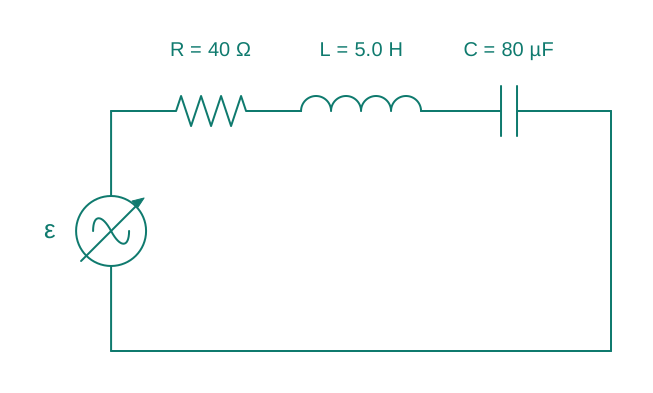
Fig. 7.21 – Series LCR circuit with a variable-frequency source.
7.12 Check Your Concepts
An alternating current has an average value of zero over one complete cycle, yet it heats a resistor. Explain, in terms of the quantity on which Joule heating depends, why this is possible.
In a pure inductor the current lags the applied voltage by π/2, while in a pure capacitor the current leads by π/2. Explain physically why an inductor and a capacitor produce opposite phase shifts.
“A pure inductor and a pure capacitor both oppose and limit an alternating current, yet neither dissipates any average power.” Explain why this statement is correct, referring to the phase relationship in each case.
A bulb is connected in series with a capacitor across an ac supply. State and justify what happens to the brightness of the bulb when (a) the supply frequency is increased, and (b) the capacitance is decreased.
Why can resonance not occur in a circuit that contains only a resistor and an inductor (RL), whereas it can occur in a series LCR circuit? Explain in terms of the voltages across the reactive elements.
A step-up transformer raises 220 V to 22000 V. Explain how this is consistent with the law of conservation of energy, and state what happens to the current.
Electrical energy is transmitted over long distances at very high voltage. (a) Why is high voltage used? (b) Why must the transmission be by alternating current rather than direct current for this scheme to be practical?
Explain the term wattless current. In which kind of ac circuit does such a current flow, and why is no average power dissipated even though the current is non-zero?
A series LCR circuit is driven exactly at its resonant frequency. Predict, with reasons, (a) the phase angle between the source voltage and the current, and (b) the combined rms voltage across the inductor–capacitor (LC) pair.
7.13 Practice with Numericals
An ac source has a peak voltage of 170 V and a frequency of 50 Hz. (a) Write the expression for the instantaneous voltage as a function of time. (b) Find the rms value of the voltage.
A 250 Ω resistor is connected to a 200 V (rms), 50 Hz ac supply. Find (a) the rms current, (b) the peak current, and (c) the average power dissipated in the resistor.
A coil of inductance 0.80 H and negligible resistance is connected to a 120 V (rms), 50 Hz supply. Find (a) the inductive reactance, (b) the rms current, and (c) the average power consumed by the coil. (Take π = 3.14.)
A 40 µF capacitor is connected to a 200 V (rms), 50 Hz supply. Find (a) the capacitive reactance and (b) the rms current. (c) If the frequency is doubled, what is the new rms current? (Take π = 3.14.)
A series LCR circuit has R = 12 Ω, inductive reactance X_L = 20 Ω, and capacitive reactance X_C = 4 Ω, connected to a 240 V (rms) supply. Find (a) the impedance, (b) the rms current, (c) the phase angle between the voltage and the current, (d) the power factor, and (e) the average power dissipated.
A series LCR circuit has L = 2.0 H and C = 8.0 µF. Find (a) the resonant angular frequency and (b) the resonant frequency in hertz. (Take π = 3.14.)
An ideal transformer has 500 turns in its primary and 100 turns in its secondary. The primary is connected to a 220 V ac supply. (a) Find the secondary voltage. (b) If the secondary delivers a current of 2.0 A, find the primary current. (c) Is this a step-up or a step-down transformer?
A power of 20 kW is to be transmitted through a line of total resistance 5.0 Ω at unity power factor. Compare the power lost as heat in the line when the power is transmitted at (a) 200 V and (b) 2000 V, and comment on the result.