Chapter 5: Magnetism and Matter
More than two thousand years ago, me shaped and miners in a region of ancient Greece called Magnesia noticed something strange. Certain dark, heavy stones found in the ground could pull small pieces of iron towards them — with no string, no push, no visible contact. These naturally magnetic stones, known today as lodestones, gave us the very word “magnet,” and records of them go back to about 600 BC.
Centuries later, Chinese navigators made an even more remarkable discovery. A sliver of lodestone, floated on water or balanced on a pivot, would slowly swing around and settle pointing in the north–south direction — every single time, anywhere on Earth. By around the eleventh century, this “south-pointing needle” was guiding ships across open seas, long before anyone could explain why it worked. Sailors trusted their lives to a stone whose behaviour was a complete mystery.
Think about what this means: the Earth itself must somehow be acting on the stone. A planet behaving like a magnet, an ordinary rock pulling iron, and a needle that always knows its direction — these puzzles waited centuries for an explanation. In this chapter, we study magnetism as a subject in its own right and finally answer what those ancient sailors could not.
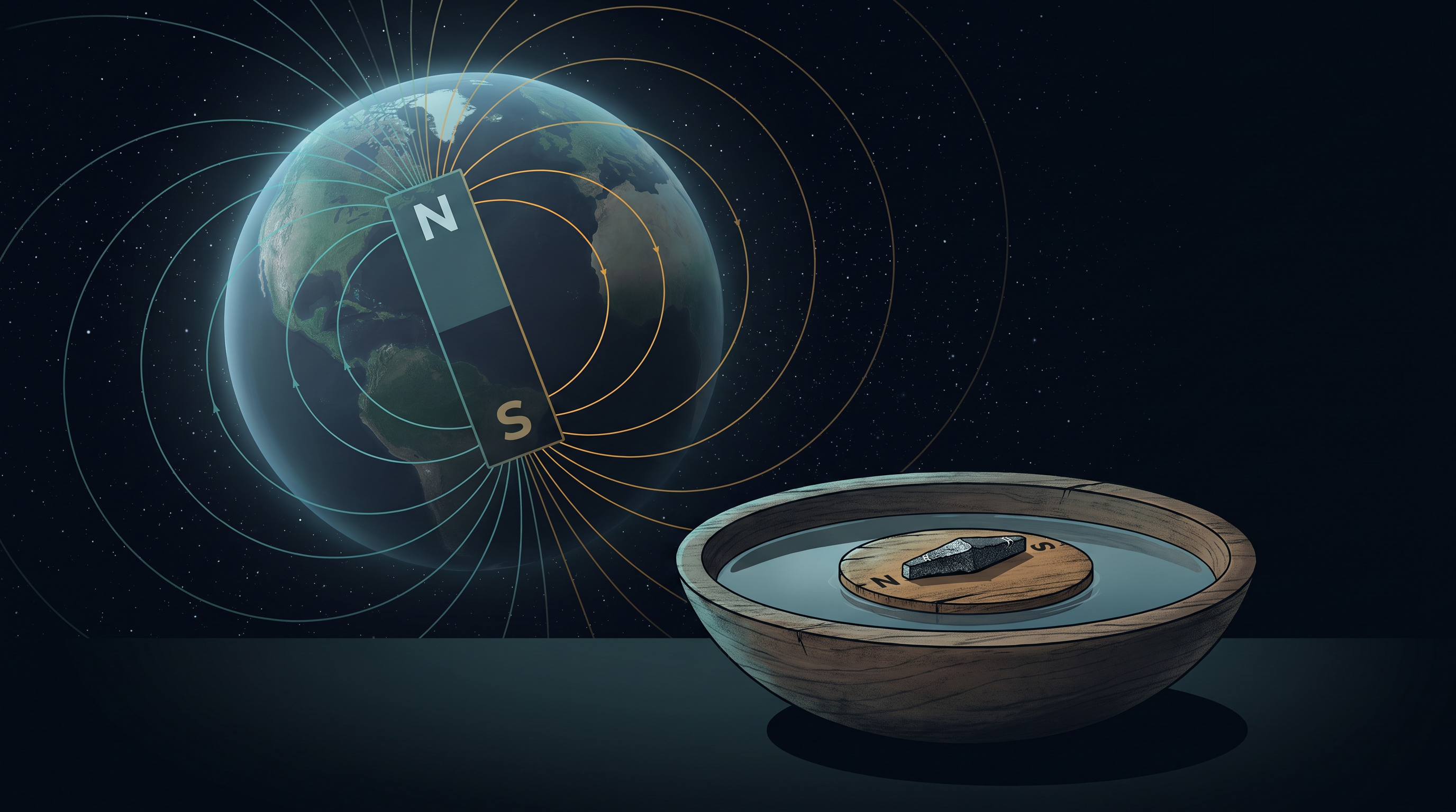
Fig. 5.0 – A floating lodestone compass aligned by Earth’s magnetic field.
By the end of this chapter, you will be able to answer every one of these questions.
5.1 Introduction
Magnetic phenomena are truly universal in nature. Enormous, distant galaxies carry magnetic fields spread across thousands of light years. The tiny, invisible atoms that make up all matter have magnetic effects hidden inside them. Even human beings and animals are permeated through and through by a host of magnetic fields arising from a variety of sources.
The Earth’s own magnetism is far older than we are — it predates human evolution itself. As we saw in the opening story of this chapter, naturally magnetic ore was known in the Greek region of Magnesia as early as 600 BC, and it is from the name of this place that the word magnet comes.
In the previous chapter, we learned something remarkable: moving charges, or electric currents, produce magnetic fields. In other words, electricity and magnetism are not two separate subjects but deeply connected ones. This discovery was made in the early part of the nineteenth century, and the credit for it goes to Oersted, Ampere, Biot and Savart, among others.
In the present chapter, we change our point of view. Instead of treating magnetism as something produced by currents, we take a look at magnetism as a subject in its own right — magnets, magnetic materials, and the laws that govern them.
Let us first collect some commonly known ideas about magnetism. You have probably met most of these in earlier classes, but they now become the starting points of a deeper study.
- The Earth behaves as a magnet. Its magnetic field points approximately from the geographic south to the geographic north. This is why the Earth can act on compass needles everywhere on its surface, as shown in Fig. 5.1a.
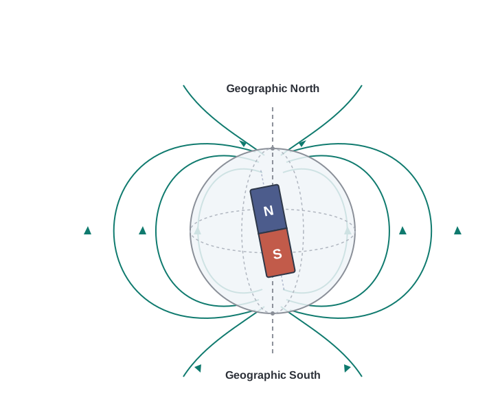
Fig. 5.1a – Earth’s magnetic field and its equivalent internal bar magnet.
- When a bar magnet is suspended freely — say, hung by a light thread so it can rotate — it always comes to rest pointing in the north–south direction. The tip that points towards the geographic north is called the north pole of the magnet, and the tip that points towards the geographic south is called its south pole.
Like poles repel and unlike poles attract. If the north poles (or the south poles) of two magnets are brought close together, there is a repulsive force between them. Conversely, there is an attractive force between the north pole of one magnet and the south pole of the other.
Magnetic poles always come in pairs — we cannot isolate the north pole or the south pole of a magnet. If a bar magnet is broken into two halves, we do not get a separate north piece and a separate south piece. Instead, we get two similar, complete bar magnets, each with its own north and south pole, though with somewhat weaker properties. This is strikingly different from electric charge: a positive charge can exist entirely on its own, but an isolated magnetic pole — called a magnetic monopole — does not exist.
It is possible to make magnets artificially out of iron and its alloys. This is how the magnets used in everyday devices are manufactured.
These five simple observations raise deep questions: why do poles always come in pairs? Why does the Earth act like a magnet? This chapter builds the physics needed to answer them. We begin with a description of a bar magnet and its behaviour in an external magnetic field. We then describe Gauss’s law of magnetism — the magnetic counterpart of the Gauss’s law you studied in electrostatics. Finally, we describe how materials can be classified on the basis of their magnetic properties, studying three families of materials: diamagnetic, paramagnetic and ferromagnetic substances.
5.2 The Bar Magnet
We begin our study with the simplest and most familiar magnet of all: the bar magnet. A classic way to “see” what a magnet does to the space around it is to sprinkle iron filings on a sheet of glass placed over a short bar magnet. When the glass is tapped gently, the filings arrange themselves into a striking pattern of curved lines, as shown in Fig. 5.2.
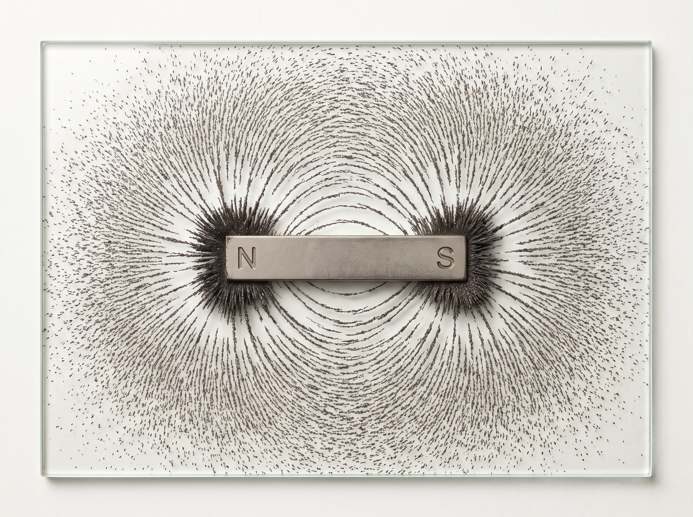
Fig. 5.2 – Iron filings tracing the magnetic field of a bar magnet.
Why do the filings do this? Each tiny filing becomes a small magnet in the field of the bar magnet and aligns itself along the local direction of the field. Together, thousands of filings trace out the shape of the magnetic field.
The pattern tells us something important: the filings crowd most densely near the two ends of the magnet. This suggests that the magnet has two poles, playing a role similar to the positive and negative charges of an electric dipole (which you studied in Chapter 1). As mentioned in the introduction, one pole is designated the North pole and the other the South pole, and when the magnet is suspended freely, these poles point approximately towards the geographic north and south, respectively.
Here is a clue worth noting early: a very similar pattern of iron filings is observed around a current-carrying solenoid. A coil of wire carrying current behaves, from the outside, just like a bar magnet. We will make this connection precise in Section 5.2.2.
5.2.1 The magnetic field lines
The pattern of iron filings permits us to plot the magnetic field lines. Field lines are not real physical threads in space — they are a visual and intuitive way of representing the magnetic field, exactly as electric field lines represented the electric field in electrostatics. Figure 5.3 shows the field lines of (a) a bar magnet and (b) a current-carrying finite solenoid; for comparison, the electric field lines of an electric dipole are displayed in Fig. 5.3(c). Notice how, at large distances, all three patterns look very similar.
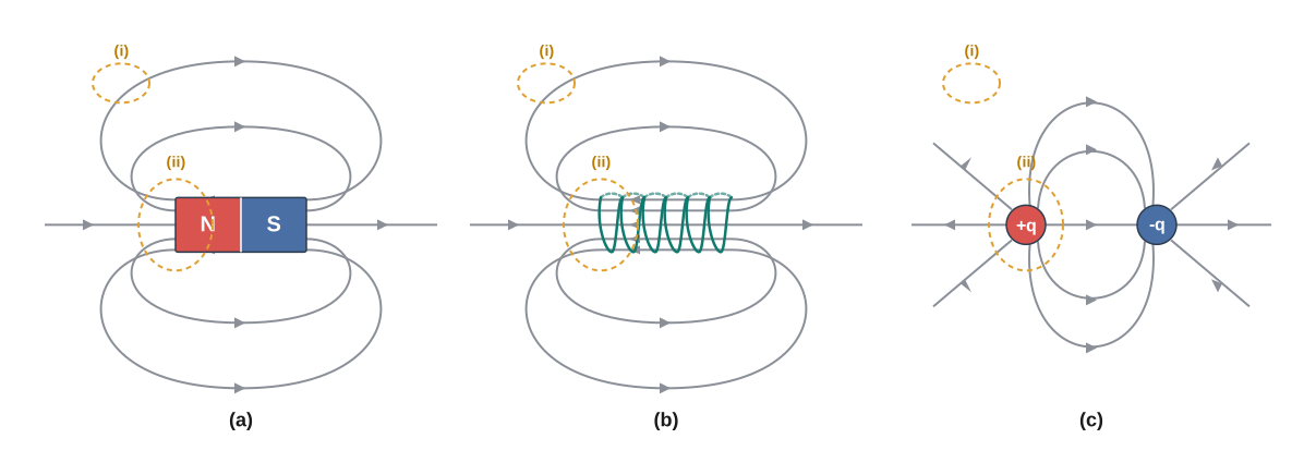
Fig. 5.3 – Field lines of (a) a bar magnet, (b) a finite solenoid, and (c) an electric dipole.
The magnetic field lines have the following properties. Compare each one carefully with what you know about electric field lines — the differences are as important as the similarities.
(i) Magnetic field lines form continuous closed loops. The field lines of a magnet (or a solenoid) never begin or end anywhere; each line closes on itself. This is unlike the electric dipole, where field lines begin on the positive charge and end on the negative charge (or escape to infinity). You can see this clearly in Fig. 5.3: in (a) and (b) the lines loop through the body of the magnet or solenoid and close, while in (c) they start and stop on the charges.
(ii) The tangent gives the direction of the field. The tangent to a field line at a given point represents the direction of the net magnetic field \(\vec{B}\) at that point. If a tiny compass needle is placed there, it aligns along this tangent.
(iii) Line density gives the strength of the field. The larger the number of field lines crossing per unit area, the stronger the magnitude of the magnetic field \(\vec{B}\). In Fig. 5.3(a), the lines are packed more closely around region (ii) than around region (i), so \(\vec{B}\) is larger around region (ii).
(iv) Field lines never intersect. Two magnetic field lines cannot cross each other. If they did, there would be two different tangents — and hence two different directions of \(\vec{B}\) — at the point of intersection. But the magnetic field at a point can have only one direction, so intersection is impossible.
How does one actually plot magnetic field lines in the laboratory? One can plot them in a variety of ways. One simple way is to place a small magnetic compass needle at various positions around the magnet and note its orientation at each place. The needle’s alignment gives the direction of the magnetic field at that point, and joining up these directions point by point traces out the field lines in space.
5.2.2 Bar magnet as an equivalent solenoid
In the previous chapter (Section 4.9), we explained how a current loop acts as a magnetic dipole: a loop of area \(A\) carrying current \(I\) has a magnetic moment of magnitude \(m = IA\) (and \(m = NIA\) for \(N\) turns), directed along the axis of the loop by the right-hand rule.
We also mentioned Ampere’s hypothesis there — the bold idea that all magnetic phenomena, including those of ordinary magnets, can be explained in terms of circulating currents.
The resemblance between the magnetic field lines of a bar magnet and those of a solenoid, seen in Figs. 5.3(a) and (b), suggests a powerful picture: a bar magnet may be thought of as a large number of circulating currents stacked together, in analogy with the many current-carrying turns of a solenoid.
This picture immediately explains a puzzle from the introduction. Cutting a bar magnet in half is like cutting a solenoid across its middle: we simply get two smaller solenoids, each still a complete solenoid with current circulating around it, and each therefore with its own north and south face — only with weaker magnetic properties. The field lines remain continuous, emerging from one face of each smaller solenoid and entering the other face. No amount of cutting can ever produce an isolated pole, because every piece, however small, still contains complete current loops.
One can test the bar magnet–solenoid analogy experimentally: move a small compass needle around a bar magnet, and then around a current-carrying finite solenoid, and note that the deflections of the needle are similar in both cases.
To make this analogy more firm, we may calculate the axial field of a finite solenoid — the field at a point P on its axis — as depicted in Fig. 5.4(a). Here the solenoid has length \(2l\), radius \(a\), and P lies at a distance \(r\) from its centre O. We can demonstrate that at large distances (\(r \gg l\) and \(r \gg a\)), this axial field resembles that of a bar magnet.
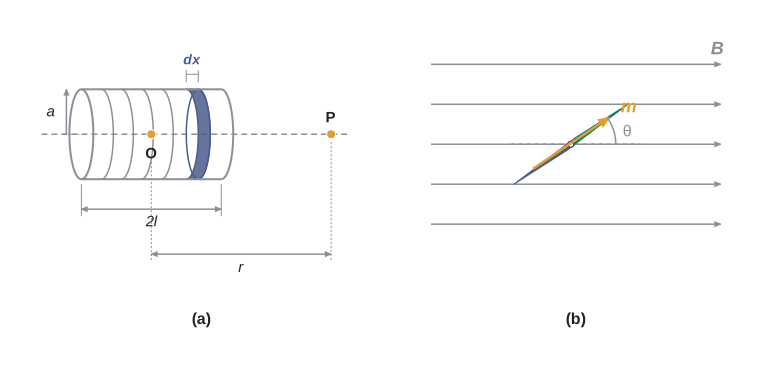
Fig. 5.4 – (a) Geometry of a finite solenoid and (b) a dipole in a uniform field.
The magnitude of the field at point P due to the solenoid works out to be
\[B = \frac{\mu_0}{4\pi}\,\frac{2m}{r^3} \tag{5.1}\]
Here \(m\) is the total magnetic moment of the solenoid, \(r\) is the distance of P from the centre of the solenoid (in metres, m), \(\mu_0\) is the permeability of free space (\(\mu_0 = 4\pi \times 10^{-7}\) T m A\(^{-1}\)), and \(B\) is in tesla (T). Notice the \(1/r^3\) dependence — the field of a dipole falls off with the cube of the distance, faster than the \(1/r^2\) fall of the field of a single point charge in electrostatics.
The significance of Eq. (5.1) is this: it is also the far axial magnetic field of a bar magnet, which one may obtain experimentally. Thus, a bar magnet and a solenoid produce similar magnetic fields. The magnetic moment of a bar magnet is therefore defined to be equal to the magnetic moment of an equivalent solenoid — one that produces the same magnetic field.
5.2.3 The dipole in a uniform magnetic field
Having established what a bar magnet is, we now ask how it behaves when placed in an external magnetic field. Let us place a small compass needle of known magnetic moment \(\vec{m}\) in a uniform magnetic field \(\vec{B}\) and allow it to oscillate. This arrangement is shown in Fig. 5.4(b).
The torque on the needle is [see Eq. (4.23) of the previous chapter],
\[\vec{\tau} = \vec{m} \times \vec{B} \tag{5.2}\]
In magnitude,
\[\tau = mB\sin\theta\]
Here \(\tau\) is the restoring torque (SI unit: N m), \(m\) is the magnitude of the magnetic moment (A m\(^2\), equivalently J T\(^{-1}\)), \(B\) is the magnetic field (T), and \(\theta\) is the angle between \(\vec{m}\) and \(\vec{B}\).
Why “restoring”? Whenever the needle is turned away from the field direction, this torque acts to rotate it back towards alignment with \(\vec{B}\) — just as gravity pulls a displaced pendulum back towards the vertical. If disturbed, the needle therefore oscillates about the field direction.
This is precisely why a freely suspended magnet, or a compass needle, always settles pointing north–south. The Earth’s magnetic field exerts a torque \(\vec{m} \times \vec{B}\) on the needle whenever its moment is not aligned with the field; the needle swings, loses energy to friction, and finally comes to rest with \(\vec{m}\) along the Earth’s field — which runs approximately south to north.
Since the field exerts a torque on the dipole, work must be done by an external agent to rotate the dipole against this torque. That work gets stored as magnetic potential energy, in exactly the same way that work done against the electric torque on an electric dipole was stored as electrostatic potential energy (Chapter 1).
The magnetic potential energy \(U_m\) is obtained by integrating the torque over the angle turned:
\[U_m = \int \tau(\theta)\, d\theta\]
\[= \int mB \sin\theta \, d\theta = -mB\cos\theta\]
\[= -\vec{m}\cdot\vec{B} \tag{5.3}\]
The middle step uses the standard integral \(\int \sin\theta \, d\theta = -\cos\theta\), and the last step recognises that \(mB\cos\theta\) is exactly the dot product \(\vec{m}\cdot\vec{B}\).
You may ask: an indefinite integral should carry a constant of integration — where has it gone? We have emphasised in Chapter 2 that the zero of potential energy can be fixed at one’s convenience. Taking the constant of integration to be zero amounts to fixing the zero of potential energy at \(\theta = 90°\), i.e., when the needle is perpendicular to the field.
With this convention, Eq. (5.3) tells us the whole energy story of the dipole:
- Potential energy is minimum, \(U_m = -mB\), at \(\theta = 0°\) (moment parallel to field). This is the most stable position.
- Potential energy is maximum, \(U_m = +mB\), at \(\theta = 180°\) (moment antiparallel to field). This is the most unstable position.
In examinations, this idea is typically tested through numericals asking for the torque at a given angle, the work done in rotating a magnet from one orientation to another (\(W = U_{final} - U_{initial}\)), or identification of stable/unstable equilibrium positions. Keep the sign convention of Eq. (5.3) firmly in mind — most errors come from dropped minus signs.
5.2.4 The electrostatic analog
If you place Eqs. (5.1), (5.2) and (5.3) side by side with the corresponding equations for the electric dipole from Chapter 1, a beautiful pattern emerges: the two sets of equations are identical in form. The magnetic field at large distances due to a bar magnet of magnetic moment \(\vec{m}\) can be obtained from the equations for the electric field of an electric dipole of dipole moment \(\vec{p}\), simply by making the following replacements:
\[\vec{E} \rightarrow \vec{B}, \quad \vec{p} \rightarrow \vec{m}, \quad \frac{1}{4\pi\varepsilon_0} \rightarrow \frac{\mu_0}{4\pi}\]
This is a translation dictionary between electrostatics and magnetism. Any far-field result you derived for the electric dipole can be instantly rewritten for the magnetic dipole — no fresh derivation needed.
In particular, we can write down the equatorial field (\(\vec{B}_E\)) of a bar magnet — the field at a point on the perpendicular bisector of the magnet — at a distance \(r\), for \(r \gg l\), where \(l\) is the size of the magnet:
\[\vec{B}_E = -\frac{\mu_0 \vec{m}}{4\pi r^3} \tag{5.4}\]
The minus sign says that on the equatorial line, the field points opposite to the magnetic moment \(\vec{m}\), exactly as the equatorial electric field of an electric dipole points opposite to \(\vec{p}\).
Likewise, the axial field (\(\vec{B}_A\)) of a bar magnet for \(r \gg l\) is:
\[\vec{B}_A = \frac{\mu_0}{4\pi}\,\frac{2\vec{m}}{r^3} \tag{5.5}\]
Equation (5.5) is just Eq. (5.1) in vector form. On the axis, the field is parallel to \(\vec{m}\) and is twice as strong as the equatorial field at the same distance. The condition \(r \gg l\) (“short dipole” or “far field”) is essential — these compact formulas hold only far from the magnet compared with its own size, and dropping this condition is a common examination error.
Table 5.1 summarises the analogy between electric and magnetic dipoles. As shown in the table, every electrostatic dipole quantity has a magnetic twin.
Table 5.1 – The Dipole Analogy
| Electrostatics | Magnetism | |
|---|---|---|
| \(1/\varepsilon_0\) | \(\mu_0\) | |
| Dipole moment | \(\vec{p}\) | \(\vec{m}\) |
| Equatorial field for a short dipole | \(-\vec{p}/4\pi\varepsilon_0 r^3\) | \(-\mu_0\vec{m}/4\pi r^3\) |
| Axial field for a short dipole | \(2\vec{p}/4\pi\varepsilon_0 r^3\) | \(\mu_0 2\vec{m}/4\pi r^3\) |
| External field: torque | \(\vec{p} \times \vec{E}\) | \(\vec{m} \times \vec{B}\) |
| External field: energy | \(-\vec{p}\cdot\vec{E}\) | \(-\vec{m}\cdot\vec{B}\) |
In numerical problems, Eqs. (5.4) and (5.5) are most often tested by asking for the field at a given distance on the axis or the equator, or by comparing the two (“at what point is the field the same…?”). Remember the factor of 2 and the direction reversal on the equatorial line.
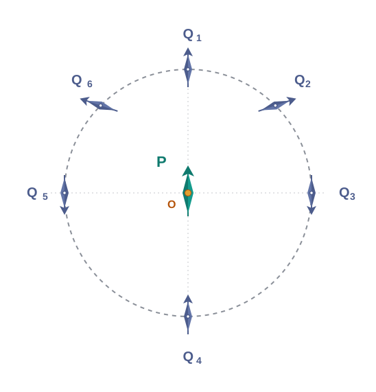
Figure 5.5 shows a small magnetised needle P placed at a point O. The arrow shows the direction of its magnetic moment. The other arrows show different positions (and orientations of the magnetic moment) of another identical magnetised needle Q.
(a) In which configuration is the system not in equilibrium?
(b) In which configuration is the system in (i) stable, and (ii) unstable equilibrium?
(c) Which configuration corresponds to the lowest potential energy among all the configurations shown?
[Caption:] Fig. 5.5 – A magnetic needle P and an identical needle Q at various positions. [/Caption:]
Solution
The potential energy of the configuration arises due to the potential energy of one dipole (say, Q) in the magnetic field due to the other (P). Use the result that the field due to P is given by the expressions [Eqs. (5.4) and (5.5)]:
\[\vec{B}_P = -\frac{\mu_0}{4\pi}\,\frac{\vec{m}_P}{r^3} \quad \text{(on the normal bisector)}\]
\[\vec{B}_P = \frac{\mu_0}{4\pi}\,\frac{2\,\vec{m}_P}{r^3} \quad \text{(on the axis)}\]
where \(\vec{m}_P\) is the magnetic moment of the dipole P.
Equilibrium is stable when \(\vec{m}_Q\) is parallel to \(\vec{B}_P\), and unstable when it is anti-parallel to \(\vec{B}_P\). For instance, for the configuration Q\(_3\), for which Q is along the perpendicular bisector of the dipole P, the magnetic moment of Q is parallel to the magnetic field at position 3. Hence Q\(_3\) is stable.
Thus,
PQ\(_1\) and PQ\(_2\)
- PQ\(_3\), PQ\(_6\) (stable); (ii) PQ\(_5\), PQ\(_4\) (unstable)
PQ\(_6\)
5.3 Magnetism and Gauss’s Law
In Chapter 1, we studied Gauss’s law for electrostatics: the electric flux through a closed surface is proportional to the total charge enclosed by it. We now ask the natural question — is there a corresponding law for magnetism? The answer turns out to be yes, and it is short, elegant, and packed with physical meaning.
Look again at the electric dipole in Fig. 5.3(c). For the closed surface labelled (i), the number of field lines leaving the surface is equal to the number of lines entering it. This is consistent with the fact that no net charge is enclosed by that surface. However, in the same figure, for the closed surface (ii), there is a net outward flux, because this surface does enclose a net (positive) charge.
The situation is radically different for magnetic fields, which are continuous and form closed loops. Examine the Gaussian surfaces labelled (i) or (ii) in Fig. 5.3(a) or Fig. 5.3(b). Both cases visually demonstrate the same thing: every field line that leaves the surface also comes back and enters it, because each line is a closed loop. The number of magnetic field lines leaving the surface is balanced by the number of lines entering it. The net magnetic flux is zero for both the surfaces — and this is true for any closed surface whatsoever, however oddly shaped, wherever placed.
Let us express this precisely. Consider a small vector area element \(\Delta\vec{S}\) of a closed surface S, as in Fig. 5.6. Recall from Chapter 1 that an area element is treated as a vector whose direction is along the outward normal \(\hat{n}\) to the surface.
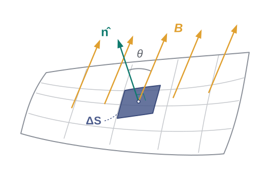
Fig. 5.6 – Magnetic flux through a small area element.
The magnetic flux through \(\Delta\vec{S}\) is defined as
\[\Delta\phi_B = \vec{B}\cdot\Delta\vec{S}\]
where \(\vec{B}\) is the field at \(\Delta\vec{S}\). Flux, loosely speaking, counts how much of the field “flows through” the little area; the dot product automatically takes care of the angle between the field and the surface. The SI unit of magnetic flux is the weber (Wb), where \(1\ \text{Wb} = 1\ \text{T m}^2\).
Now we divide the entire closed surface S into many small area elements and calculate the individual flux through each. The net flux \(\phi_B\) is the sum over all of them:
\[\phi_B = \sum_{\text{'all'}} \Delta\phi_B = \sum_{\text{'all'}} \vec{B}\cdot\Delta\vec{S} = 0 \tag{5.6}\]
where ‘all’ stands for ‘all area elements \(\Delta\vec{S}\)’ of the closed surface.
Compare this with Gauss’s law of electrostatics. The flux through a closed surface in that case is given by
\[\sum \vec{E}\cdot\Delta\vec{S} = \frac{q}{\varepsilon_0}\]
where \(q\) is the electric charge enclosed by the surface.
The contrast is striking. In electrostatics, the right-hand side can be non-zero, because electric charges — the sources and sinks on which field lines begin and end — can be enclosed by a surface. In magnetism, the right-hand side is always zero. The difference between Gauss’s law of magnetism and that of electrostatics is a reflection of the fact that isolated magnetic poles (also called monopoles) are not known to exist. There are no sources or sinks of \(\vec{B}\). The simplest magnetic element is a dipole or a current loop, and all magnetic phenomena can be explained in terms of an arrangement of dipoles and/or current loops.
Thus, Gauss’s law for magnetism is:
This law is the mathematical statement of the fact you have now met three times in this chapter — as the impossibility of isolating a pole by cutting a magnet, as the closed-loop property of field lines, and now as a flux law for any closed surface. All three are one and the same physical truth.
In exams, this law appears in two common ways: conceptual questions (“why is the net magnetic flux through a closed surface zero?”) and numericals where the flux through part of a closed surface is given and you must find the flux through the rest, using the fact that all contributions must add to zero.
Many of the diagrams given in Fig. 5.7 show magnetic field lines (thick lines in the figure) wrongly. Point out what is wrong with them. Some of them may describe electrostatic field lines correctly. Point out which ones.
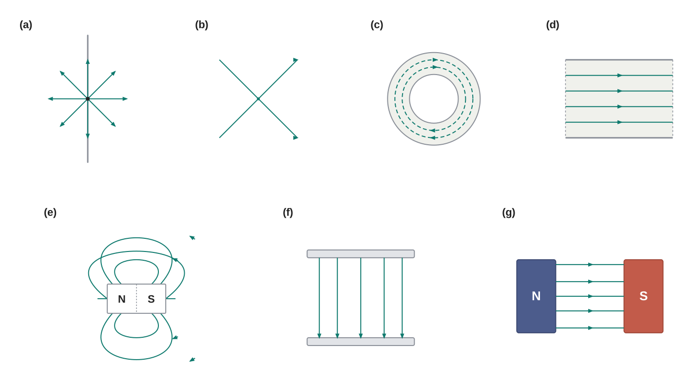
[Caption:] Fig. 5.7 – Various correct and incorrect sketches of field lines. [/Caption:]
Solution
Wrong. Magnetic field lines can never emanate from a point, as shown in the figure. Over any closed surface, the net flux of \(\vec{B}\) must always be zero, i.e., pictorially, as many field lines should seem to enter the surface as the number of lines leaving it. The field lines shown, in fact, represent the electric field of a long positively charged wire. The correct magnetic field lines circle around the straight conductor, as described in Chapter 4.
Wrong. Magnetic field lines (like electric field lines) can never cross each other, because otherwise the direction of the field at the point of intersection would be ambiguous. There is a further error in the figure: magnetostatic field lines can never form closed loops around empty space. A closed loop of a static magnetic field line must enclose a region across which a current is passing. By contrast, electrostatic field lines can never form closed loops, neither in empty space, nor when the loop encloses charges.
Right. Magnetic lines are completely confined within a toroid. Nothing is wrong here in field lines forming closed loops, since each loop encloses a region across which a current passes. Note, for clarity of the figure, only a few field lines within the toroid have been shown. Actually, the entire region enclosed by the windings contains magnetic field.
Wrong. Field lines due to a solenoid at its ends and outside cannot be so completely straight and confined; such a thing violates Ampere’s law. The lines should curve out at both ends, and meet eventually to form closed loops.
Right. These are field lines outside and inside a bar magnet. Note carefully the direction of field lines inside. Not all field lines emanate out of a north pole (or converge into a south pole). Around both the N-pole and the S-pole, the net flux of the field is zero.
Wrong. These field lines cannot possibly represent a magnetic field. Look at the upper region. All the field lines seem to emanate out of the shaded plate. The net flux through a surface surrounding the shaded plate is not zero. This is impossible for a magnetic field. The given field lines, in fact, show the electrostatic field lines around a positively charged upper plate and a negatively charged lower plate. The difference between Figs. [5.7(e) and (f)] should be carefully grasped.
Wrong. Magnetic field lines between two pole pieces cannot be precisely straight at the ends. Some fringing of lines is inevitable. Otherwise, Ampere’s law is violated. This is also true for electric field lines.
5.4 Magnetisation and Magnetic Intensity
The Earth abounds with a bewildering variety of elements and compounds. In addition, we have been synthesising new alloys, compounds and even elements. Faced with this variety, a physicist naturally asks: can we classify all these substances by their magnetic behaviour? To carry out this exercise, we first need a small vocabulary of precisely defined quantities. In the present section, we define and explain these terms; in the next section, we use them to sort all materials into three great families.
Magnetisation
We have seen that a circulating electron in an atom has a magnetic moment — it is a tiny current loop. In a bulk material, which contains an enormous number of atoms, these tiny moments add up vectorially. Depending on how they are oriented, the vector sum can cancel out to zero, or it can give a net magnetic moment which is non-zero.
To describe this on a per-volume basis, we define the magnetisation \(\vec{M}\) of a sample to be equal to its net magnetic moment per unit volume:
\[\vec{M} = \frac{\vec{m}_{net}}{V} \tag{5.7}\]
Here \(\vec{m}_{net}\) is the vector sum of all the atomic magnetic moments in the sample (unit: A m\(^2\)) and \(V\) is its volume (m\(^3\)). \(\vec{M}\) is a vector with dimensions [L\(^{-1}\) A] and is measured in units of A m\(^{-1}\).
Magnetisation answers the question “how strongly magnetised is this material, per unit volume?” — just as density answers “how much mass, per unit volume?”
The field inside a magnetised material
Now let us see how magnetisation modifies a magnetic field. Consider a long solenoid with \(n\) turns per unit length, carrying a current \(I\). In the previous chapter, the magnetic field in the interior of such a solenoid (with vacuum or air inside) was shown to be
\[B_0 = \mu_0 n I \tag{5.8}\]
where \(\mu_0\) is the permeability of vacuum, \(n\) is in turns per metre and \(I\) in amperes.
If the interior of the solenoid is now filled with a material having non-zero magnetisation, something interesting happens: the field inside becomes greater than \(B_0\). The material’s own atomic moments, aligned by the solenoid’s field, contribute an additional field of their own. The net \(\vec{B}\) field in the interior of the solenoid may then be expressed as
\[\vec{B} = \vec{B}_0 + \vec{B}_m \tag{5.9}\]
where \(\vec{B}_m\) is the field contributed by the material core. It turns out that this additional field \(\vec{B}_m\) is proportional to the magnetisation \(\vec{M}\) of the material, and is expressed as
\[\vec{B}_m = \mu_0 \vec{M} \tag{5.10}\]
where \(\mu_0\) is the same constant (permeability of vacuum) that appears in the Biot–Savart law.
Magnetic intensity H
Look carefully at what we have: the total field inside the material has two distinct causes. One part comes from the current we send through the solenoid — something we control externally. The other part comes from the response of the material itself. It is extremely convenient to give the externally controlled part its own name and symbol.
We introduce another vector field \(\vec{H}\), called the magnetic intensity, defined by
\[\vec{H} = \frac{\vec{B}}{\mu_0} - \vec{M} \tag{5.11}\]
where \(\vec{H}\) has the same dimensions as \(\vec{M}\) and is measured in units of A m\(^{-1}\).
Rearranging Eq. (5.11), the total magnetic field \(\vec{B}\) is written as
\[\vec{B} = \mu_0(\vec{H} + \vec{M}) \tag{5.12}\]
Let us repeat our defining procedure in words, because this partition is the key idea of the section. We have divided the contribution to the total magnetic field inside the sample into two parts: one, due to external factors such as the current in the solenoid — this is represented by \(\vec{H}\); the other, due to the specific nature of the magnetic material — namely \(\vec{M}\).
This is closely parallel to what you did with dielectrics in electrostatics (Chapter 2): there, the applied field polarised the dielectric, and the material’s polarisation modified the net field inside. Here, the applied field magnetises the material, and the magnetisation modifies the net field inside.
Susceptibility and permeability
The material’s response \(\vec{M}\) is not independent of the external influence — it can be influenced by external factors. For a large class of materials, this influence is mathematically simple: the magnetisation is directly proportional to the magnetic intensity,
\[\vec{M} = \chi \vec{H} \tag{5.13}\]
where \(\chi\) (the Greek letter chi), a dimensionless quantity, is appropriately called the magnetic susceptibility. It is a measure of how a magnetic material responds to an external field — literally, how “susceptible” the material is to becoming magnetised.
The sign of \(\chi\) immediately sorts materials into classes. \(\chi\) is small and positive for materials which are called paramagnetic — their magnetisation supports the external field. \(\chi\) is small and negative for materials which are termed diamagnetic — in this latter case, \(\vec{M}\) and \(\vec{H}\) are opposite in direction, so the material weakly opposes the field. We will study both classes, and a third dramatic one, in Section 5.5.
From Eqs. (5.12) and (5.13) we obtain, by substituting \(\vec{M} = \chi\vec{H}\):
\[\vec{B} = \mu_0(1 + \chi)\vec{H} \tag{5.14}\]
\[= \mu_0\,\mu_r\,\vec{H}\]
\[= \mu\,\vec{H} \tag{5.15}\]
where \(\mu_r = 1 + \chi\) is a dimensionless quantity called the relative magnetic permeability of the substance. It is the analog of the dielectric constant in electrostatics — it tells us by what factor the material multiplies the field compared to vacuum.
The magnetic permeability of the substance is \(\mu\), and it has the same dimensions and units as \(\mu_0\):
\[\mu = \mu_0\mu_r = \mu_0(1 + \chi)\]
Note that the three quantities \(\chi\), \(\mu_r\) and \(\mu\) are interrelated, and only one of them is independent. Given any one, the other two may be easily determined. In numerical problems, you will often be given one of these and asked for the others — the chains \(\mu_r = 1 + \chi\) and \(\mu = \mu_0\mu_r\) are all you need.
5.5 Magnetic Properties of Materials
The vocabulary developed in the previous section now pays off. Using the susceptibility \(\chi\), we can classify every material into one of three great families of magnetic behaviour.
A material is diamagnetic if \(\chi\) is negative, paramagnetic if \(\chi\) is positive and small, and ferromagnetic if \(\chi\) is large and positive. A glance at Table 5.2 gives one a better feeling for these materials. Here \(\varepsilon\) is a small positive number introduced to quantify paramagnetic materials.
Table 5.2
| Diamagnetic | Paramagnetic | Ferromagnetic |
|---|---|---|
| \(-1 \le \chi < 0\) | \(0 < \chi < \varepsilon\) | \(\chi \gg 1\) |
| \(0 \le \mu_r < 1\) | \(1 < \mu_r < 1 + \varepsilon\) | \(\mu_r \gg 1\) |
| \(\mu < \mu_0\) | \(\mu > \mu_0\) | \(\mu \gg \mu_0\) |
Read the table as a story: diamagnetic materials weakly oppose an applied field (\(\mu\) slightly less than \(\mu_0\)), paramagnetic materials weakly support it (\(\mu\) slightly more than \(\mu_0\)), and ferromagnetic materials support it enormously (\(\mu \gg \mu_0\)). Next, we describe these three families in some detail.
5.5.1 Diamagnetism
Diamagnetic substances are those which have a tendency to move from the stronger to the weaker part of an external magnetic field. In other words, unlike the way a magnet attracts metals like iron, it would repel a diamagnetic substance.
Figure 5.8(a) shows a bar of diamagnetic material placed in an external magnetic field. The field lines are repelled or expelled, and the field inside the material is reduced. In most cases, this reduction is slight, being about one part in \(10^5\). When placed in a non-uniform magnetic field, the bar will tend to move from the region of high field to the region of low field.
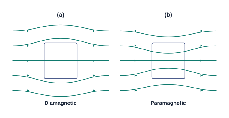
Fig. 5.8 – Magnetic field lines near (a) diamagnetic and (b) paramagnetic bars.
Why should any material oppose a magnetic field? The simplest explanation for diamagnetism is as follows. Electrons in an atom, orbiting around the nucleus, possess orbital angular momentum. These orbiting electrons are equivalent to current-carrying loops, and thus possess orbital magnetic moment. Diamagnetic substances are the ones in which the resultant magnetic moment of an atom is zero — the moments of the various electrons cancel out.
When a magnetic field is applied, this balance is disturbed. Those electrons having orbital magnetic moment in the same direction as the field slow down, and those in the opposite direction speed up. This happens due to induced currents, in accordance with Lenz’s law, which you will study in Chapter 6 — the induced effect always opposes the change that causes it. Thus, the substance develops a small net magnetic moment in the direction opposite to that of the applied field, and hence there is repulsion.
Some diamagnetic materials are bismuth, copper, lead, silicon, nitrogen (at STP), water and sodium chloride.
An important subtlety: diamagnetism is present in all substances, because every substance has orbiting electrons. However, the effect is so weak that in most materials it gets overshadowed by other, stronger effects like paramagnetism and ferromagnetism. We only “see” diamagnetism in materials that have nothing stronger to hide it.
The most exotic diamagnetic materials are superconductors. These are metals cooled to very low temperatures, which exhibit both perfect conductivity and perfect diamagnetism. Here the field lines are completely expelled from the material — not merely reduced by one part in \(10^5\), but pushed out entirely. For a superconductor, \(\chi = -1\) and \(\mu_r = 0\): it is the extreme end of the diamagnetic range in Table 5.2.
A superconductor therefore repels a magnet and — by Newton’s third law — is repelled by the magnet. The phenomenon of perfect diamagnetism in superconductors is called the Meissner effect, after the name of its discoverer.
5.5.2 Paramagnetism
Paramagnetic substances are those which get weakly magnetised when placed in an external magnetic field. They have a tendency to move from a region of weak magnetic field to a region of strong magnetic field — i.e., they get weakly attracted to a magnet. Their behaviour is opposite in sense to diamagnetism, but comparable in weakness.
The microscopic picture is quite different from the diamagnetic case. The individual atoms (or ions or molecules) of a paramagnetic material possess a permanent magnetic dipole moment of their own — the electronic moments inside each atom do not fully cancel. So why isn’t every paramagnetic material a magnet already? On account of the ceaseless random thermal motion of the atoms, the moments point in all directions and no net magnetisation is seen.
In the presence of an external field \(\vec{B}_0\) which is strong enough, and at low temperatures, the individual atomic dipole moments can be made to align and point in the same direction as \(\vec{B}_0\). Alignment is a tug-of-war: the field tries to line the dipoles up, while thermal agitation tries to randomise them. A stronger field or a lower temperature tips the contest in favour of alignment.
Figure 5.8(b) shows a bar of paramagnetic material placed in an external field. The field lines get concentrated inside the material, and the field inside is enhanced. In most cases, this enhancement is slight, being about one part in \(10^5\). When placed in a non-uniform magnetic field, the bar will tend to move from the weak-field region to the strong-field region — notice in Fig. 5.8 how this is exactly opposite to the diamagnetic bar of part (a).
Some paramagnetic materials are aluminium, sodium, calcium, oxygen (at STP) and copper chloride.
So we can now answer a question raised at the start of this chapter. Copper, water and aluminium are not indifferent to a magnet. Copper and water are diamagnetic — feebly repelled; aluminium is paramagnetic — feebly attracted. Every material responds to a magnetic field; it is only that these responses are about a hundred thousand times weaker than that of iron, and so escape our notice in everyday life.
For a paramagnetic material, both \(\chi\) and \(\mu_r\) depend not only on the material but also (in a simple fashion) on the sample temperature. As the field is increased or the temperature is lowered, the magnetisation increases, until it reaches the saturation value, at which point all the dipoles are perfectly aligned with the field. Beyond saturation, no further increase of magnetisation is possible — there is nothing left to align.
5.5.3 Ferromagnetism
Ferromagnetic substances are those which get strongly magnetised when placed in an external magnetic field. They have a strong tendency to move from a region of weak magnetic field to a region of strong magnetic field — i.e., they get strongly attracted to a magnet. This is the familiar, dramatic magnetism of everyday experience: iron filings leaping onto a magnet.
The individual atoms (or ions or molecules) in a ferromagnetic material possess a dipole moment, just as in a paramagnetic material. However — and this is the crucial new feature — they interact with one another in such a way that they spontaneously align themselves in a common direction over a macroscopic volume called a domain. The explanation of this cooperative effect requires quantum mechanics and is beyond the scope of this textbook.
Each domain has a net magnetisation. A typical domain size is 1 mm, and a domain contains about \(10^{11}\) atoms — an enormous team of atoms all pointing the same way. In the first instant, however, the magnetisation varies randomly from domain to domain, so their contributions cancel and there is no bulk magnetisation. This is shown in Fig. 5.9(a): the material as a whole is unmagnetised even though each domain individually is fully magnetised.
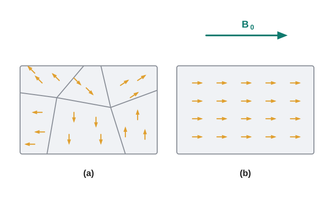
Fig. 5.9 – Ferromagnetic domains (a) randomly oriented and (b) aligned by an external field.
When we apply an external magnetic field \(\vec{B}_0\), two things happen: the domains orient themselves in the direction of \(\vec{B}_0\), and simultaneously the domains already oriented in the direction of \(\vec{B}_0\) grow in size at the expense of their neighbours. This existence of domains and their motion in \(\vec{B}_0\) are not speculations. One may observe them under a microscope after sprinkling a liquid suspension of powdered ferromagnetic substance on the sample; the motion of the suspension can be observed directly. Figure 5.9(b) shows the situation when the domains have aligned and amalgamated to form a single ‘giant’ domain.
Thus, in a ferromagnetic material the field lines are highly concentrated — compare the modest crowding of Fig. 5.8(b) with what iron does, where \(\mu_r\) can exceed 1000. In a non-uniform magnetic field, the sample tends to move towards the region of high field, and does so strongly.
We may wonder what happens when the external field is removed. Here ferromagnets split into two useful classes.
In some ferromagnetic materials, the magnetisation persists even after the field is removed. Such materials are called hard magnetic materials or hard ferromagnets. Alnico — an alloy of iron, aluminium, nickel, cobalt and copper — is one such material. The naturally occurring lodestone, the very stone from our chapter-opening story, is another. Such materials form permanent magnets, to be used among other things as compass needles.
On the other hand, there is a class of ferromagnetic materials in which the magnetisation disappears on removal of the external field. Soft iron is one such material. Appropriately enough, such materials are called soft ferromagnetic materials. They are ideal wherever we want magnetism on demand — magnetised while the field is on, neutral the moment it is off.
There are a number of elements which are ferromagnetic: iron, cobalt, nickel, gadolinium, etc. The relative magnetic permeability of ferromagnets is greater than 1000!
The ferromagnetic property depends on temperature. At a high enough temperature, a ferromagnet becomes a paramagnet: the thermal agitation grows strong enough to break up the cooperative order, and the domain structure disintegrates. (This transition temperature is called the Curie temperature of the material.) This disappearance of magnetisation with temperature is gradual, not sudden.
This completes the answer to the last of our opening questions. Iron is special because its atoms not only carry permanent magnetic moments but also cooperate, locking together into domains that can be aligned into one giant magnet. Heating destroys a magnet because thermal agitation dismantles this delicate domain order — beyond a certain temperature, proud ferromagnetic iron behaves like just another weak paramagnet.
In examinations, this section is a favourite for conceptual and assertion–reason questions: distinguishing dia-, para- and ferromagnetic behaviour from the sign and size of \(\chi\), explaining domain behaviour, contrasting hard and soft ferromagnets, and describing the effect of temperature. Table 5.2, together with the microscopic pictures above, covers nearly all of them.
5.6 Summary
The science of magnetism is old. It has been known since ancient times that magnetic materials tend to point in the north–south direction; that like magnetic poles repel and unlike ones attract; and that cutting a bar magnet in two leads to two smaller magnets, each complete with both poles. Magnetic poles cannot be isolated.
When a bar magnet of dipole moment \(\vec{m}\) is placed in a uniform magnetic field \(\vec{B}\):
- the net force on it is zero,
- the torque on it is \(\vec{\tau} = \vec{m} \times \vec{B}\),
- its potential energy is \(U_m = -\vec{m}\cdot\vec{B}\), where we choose the zero of energy at the orientation when \(\vec{m}\) is perpendicular to \(\vec{B}\).
Consider a bar magnet of size \(l\) and magnetic moment \(\vec{m}\), at a distance \(r\) from its mid-point, where \(r \gg l\). The magnetic field \(\vec{B}\) due to this bar is:
\[\vec{B} = \frac{\mu_0\vec{m}}{2\pi r^3} \quad \text{(along axis)}\]
\[= -\frac{\mu_0\vec{m}}{4\pi r^3} \quad \text{(along equator)}\]
The axial field is parallel to \(\vec{m}\) and twice as strong as the equatorial field at the same distance, which points opposite to \(\vec{m}\).
- Gauss’s law for magnetism states that the net magnetic flux through any closed surface is zero:
\[\phi_B = \sum_{\substack{\text{all area} \\ \text{elements } \Delta\vec{S}}} \vec{B}\cdot\Delta\vec{S} = 0\]
This expresses the fact that there are no sources or sinks of \(\vec{B}\) — magnetic monopoles do not exist.
- Consider a material placed in an external magnetic field \(\vec{B}_0\). The magnetic intensity is defined as
\[\vec{H} = \frac{\vec{B}_0}{\mu_0}\]
The magnetisation \(\vec{M}\) of the material is its net dipole moment per unit volume. The total magnetic field \(\vec{B}\) inside the material is
\[\vec{B} = \mu_0(\vec{H} + \vec{M})\]
- For a linear material, \(\vec{M} = \chi\vec{H}\), so that \(\vec{B} = \mu\vec{H}\), where \(\chi\) is called the magnetic susceptibility of the material. The three quantities — \(\chi\), the relative magnetic permeability \(\mu_r\), and the magnetic permeability \(\mu\) — are related as follows:
\[\mu = \mu_0\mu_r\] \[\mu_r = 1 + \chi\]
Only one of the three is independent; given any one, the other two follow.
Magnetic materials are broadly classified as diamagnetic, paramagnetic and ferromagnetic. For diamagnetic materials, \(\chi\) is negative and small; for paramagnetic materials, it is positive and small. Ferromagnetic materials have large \(\chi\).
Substances which, at room temperature, retain their ferromagnetic property for a long period of time are called permanent magnets.
Physical Quantities at a Glance
| Physical quantity | Symbol | Nature | Dimensions | Units | Remarks |
|---|---|---|---|---|---|
| Permeability of free space | \(\mu_0\) | Scalar | [MLT\(^{-2}\)A\(^{-2}\)] | T m A\(^{-1}\) | \(\mu_0/4\pi = 10^{-7}\) |
| Magnetic field, magnetic induction, magnetic flux density | \(\vec{B}\) | Vector | [MT\(^{-2}\)A\(^{-1}\)] | T (tesla) | \(10^4\) G (gauss) = 1 T |
| Magnetic moment | \(\vec{m}\) | Vector | [L\(^{-2}\)A] | A m\(^2\) | |
| Magnetic flux | \(\phi_B\) | Scalar | [ML\(^2\)T\(^{-2}\)A\(^{-1}\)] | W (weber) | W = T m\(^2\) |
| Magnetisation | \(\vec{M}\) | Vector | [L\(^{-1}\)A] | A m\(^{-1}\) | Magnetic moment / Volume |
| Magnetic intensity, magnetic field strength | \(\vec{H}\) | Vector | [L\(^{-1}\)A] | A m\(^{-1}\) | \(\vec{B} = \mu_0(\vec{H} + \vec{M})\) |
| Magnetic susceptibility | \(\chi\) | Scalar | – | – | \(\vec{M} = \chi\vec{H}\) |
| Relative magnetic permeability | \(\mu_r\) | Scalar | – | – | \(\vec{B} = \mu_0\mu_r\vec{H}\) |
| Magnetic permeability | \(\mu\) | Scalar | [MLT\(^{-2}\)A\(^{-2}\)] | T m A\(^{-1}\), N A\(^{-2}\) | \(\mu = \mu_0\mu_r\); \(\vec{B} = \mu\vec{H}\) |
5.7 Points to Ponder
A satisfactory understanding of magnetic phenomena in terms of moving charges and currents was arrived at only after 1800 AD. But the technological exploitation of the directional properties of magnets — the compass — predates this scientific understanding by two thousand years. Thus, scientific understanding is not a necessary condition for engineering applications. Ideally, science and engineering go hand-in-hand, one leading and assisting the other in tandem.
Magnetic monopoles do not exist. If you slice a magnet in half, you get two smaller magnets, never a lone pole. On the other hand, isolated positive and negative electric charges do exist. There exists a smallest unit of charge — the electronic charge, with value \(|e| = 1.6 \times 10^{-19}\) C — and all other charges are integral multiples of this smallest unit. In other words, charge is quantised. Curiously, we do not know why magnetic monopoles do not exist, or why electric charge is quantised. Both remain open questions at the foundations of physics.
A direct consequence of the fact that magnetic monopoles do not exist is that magnetic field lines are continuous and form closed loops. In contrast, the electrostatic lines of force begin on a positive charge and terminate on the negative charge (or fade out at infinity). One picture has no ends; the other always does.
A minuscule difference in the value of the magnetic susceptibility \(\chi\) yields radically different behaviour: diamagnetic versus paramagnetic. For diamagnetic materials \(\chi = -10^{-5}\), whereas \(\chi = +10^{-5}\) for paramagnetic materials. The magnitudes are the same tiny number — only the sign differs, yet one substance creeps away from a magnet while the other creeps towards it.
There exists a perfect diamagnet — namely, a superconductor. This is a metal at very low temperatures. In this case \(\chi = -1\), \(\mu_r = 0\), \(\mu = 0\): the external magnetic field is totally expelled. Interestingly, this material is also a perfect conductor. However, there exists no classical theory which ties these two properties together. A quantum-mechanical theory by Bardeen, Cooper and Schrieffer (the BCS theory) explains these effects. The BCS theory was proposed in 1957 and was eventually recognised by a Nobel Prize in Physics in 1970.
Diamagnetism is universal — it is present in all materials, since every atom has orbiting electrons. But it is weak and hard to detect if the substance is para- or ferromagnetic, because those stronger effects mask it completely.
We have classified materials as diamagnetic, paramagnetic and ferromagnetic. However, there exist additional types of magnetic material — such as ferrimagnetic, anti-ferromagnetic, spin glass, etc. — with properties which are exotic and mysterious. The three-way classification of this chapter is the beginning of the subject, not the end.
5.8 NCERT Questions
A short bar magnet placed with its axis at \(30°\) with a uniform external magnetic field of \(0.25\) T experiences a torque of magnitude equal to \(4.5 \times 10^{-2}\) J. What is the magnitude of the magnetic moment of the magnet?
A short bar magnet of magnetic moment \(m = 0.32\) J T\(^{-1}\) is placed in a uniform magnetic field of \(0.15\) T. If the bar is free to rotate in the plane of the field, which orientation would correspond to its (a) stable, and (b) unstable equilibrium? What is the potential energy of the magnet in each case?
A closely wound solenoid of 800 turns and area of cross section \(2.5 \times 10^{-4}\) m\(^2\) carries a current of \(3.0\) A. Explain the sense in which the solenoid acts like a bar magnet. What is its associated magnetic moment?
If the solenoid in Question 3 is free to turn about the vertical direction and a uniform horizontal magnetic field of \(0.25\) T is applied, what is the magnitude of the torque on the solenoid when its axis makes an angle of \(30°\) with the direction of the applied field?
A bar magnet of magnetic moment \(1.5\) J T\(^{-1}\) lies aligned with the direction of a uniform magnetic field of \(0.22\) T.
- What is the amount of work required by an external torque to turn the magnet so as to align its magnetic moment: (i) normal to the field direction, (ii) opposite to the field direction?
- What is the torque on the magnet in cases (i) and (ii)?
A closely wound solenoid of 2000 turns and area of cross-section \(1.6 \times 10^{-4}\) m\(^2\), carrying a current of \(4.0\) A, is suspended through its centre allowing it to turn in a horizontal plane.
- What is the magnetic moment associated with the solenoid?
- What is the force and torque on the solenoid if a uniform horizontal magnetic field of \(7.5 \times 10^{-2}\) T is set up at an angle of \(30°\) with the axis of the solenoid?
A short bar magnet has a magnetic moment of \(0.48\) J T\(^{-1}\). Give the direction and magnitude of the magnetic field produced by the magnet at a distance of \(10\) cm from the centre of the magnet on (a) the axis, (b) the equatorial lines (normal bisector) of the magnet.
5.9 Check Your Concepts
A bar magnet is cut into four equal pieces, first transverse to its length and then along its length. How many complete magnets are obtained? Will any piece have only a north pole? Justify your answer using the solenoid picture of a bar magnet.
Magnetic field lines and electrostatic field lines both use the tangent to indicate field direction, and neither can intersect. State the one property in which the two kinds of field lines differ fundamentally, and name the physical fact about nature that this difference reflects.
A magnetised needle placed in a uniform magnetic field experiences zero net force, yet it rotates when released from a non-aligned orientation. Explain how both statements can be true simultaneously.
Two positions of a compass needle in a uniform magnetic field correspond to zero torque: \(\theta = 0°\) and \(\theta = 180°\). A student claims both are equilibrium positions and therefore both are equally stable. Point out the error in this claim using the expression for magnetic potential energy.
A closed Gaussian surface is drawn so that it encloses only the north-pole end of a long bar magnet. A student argues that since “field lines come out of a north pole,” the net magnetic flux through this surface must be positive. Is the student correct? Explain.
The magnetic intensity \(H\) inside a current-carrying solenoid remains unchanged when its air core is replaced by a soft iron core, but the magnetic field \(B\) increases enormously. Explain why one quantity changes and the other does not.
A small bar of material X moves slowly towards the strong-field region of a non-uniform magnetic field, while an identical-looking bar of material Y moves slowly towards the weak-field region. Neither response is strong. Classify X and Y, and describe what happens to the magnetic field lines inside each bar.
- Why does a paramagnetic sample display greater magnetisation when cooled, whereas the diamagnetic response of a sample is nearly independent of temperature? (b) Why does a ferromagnet lose its ferromagnetism gradually, rather than abruptly, as it is heated?
An electromagnet used in an electric bell must lose its magnetism the instant the current stops, while a magnet used in a magnetic compass must retain its magnetism for years. Which class of ferromagnetic material is suitable for each purpose? Give one example of each.
5.10 Practice with Numericals
A short bar magnet experiences a torque of \(6.0 \times 10^{-2}\) N m when its axis makes an angle of \(60°\) with a uniform magnetic field of \(0.40\) T. Calculate (a) the magnetic moment of the magnet, and (b) the work done in rotating it from this orientation to the orientation of stable equilibrium.
A closely wound solenoid has 500 turns, each of area \(4.0 \times 10^{-4}\) m\(^2\), and carries a current of \(2.5\) A. It is placed with its axis at \(45°\) to a uniform magnetic field of \(0.30\) T. Calculate (a) the magnetic moment of the solenoid, (b) the magnitude of the torque acting on it, and (c) its potential energy in this orientation.
A short bar magnet has a magnetic moment of \(1.2\) J T\(^{-1}\). At what distance from its centre, on the axis, is the magnitude of the magnetic field equal to \(3.0 \times 10^{-5}\) T? What is the magnitude of the field at the same distance on the equatorial line?
A magnetic field of magnitude \(2.0 \times 10^{-3}\) T passes through a circular loop of radius \(7.0\) cm, making an angle of \(30°\) with the plane of the loop. Calculate the magnetic flux through the loop. If this loop is one face of a closed surface, what is the net magnetic flux through the entire closed surface?
A solenoid with 600 turns per metre carries a current of \(1.5\) A. Its core is a material of magnetic susceptibility \(\chi = 599\). Calculate (a) the magnetic intensity \(H\), (b) the magnetisation \(M\), (c) the magnetic field \(B\) inside the core, and (d) the relative permeability of the core material.
The magnetic susceptibility of a superconductor is \(\chi = -1\). A sample of a superconducting material is placed in an external magnetic intensity \(H = 5.0 \times 10^{3}\) A m\(^{-1}\). Calculate (a) the magnetisation \(M\) of the sample, and (b) the magnetic field \(B\) inside it, and state what your answer to (b) implies physically.