← Back to Subjects ororo.world

Chapter 8: Electromagnetic Waves

In the late 1880s, in a laboratory in Karlsruhe, Germany, a young physicist named Heinrich Hertz set up a curious arrangement. On one side of a darkened room he built a circuit with a tiny air gap, across which he made electric sparks jump. On the other side of the room, completely disconnected from the first, he placed a simple loop of wire with its own small gap. There was no wire joining the two, no visible link of any kind.

Each time a spark crackled across the first gap, a much fainter spark leapt across the gap in the distant loop. Something invisible had travelled across the empty room and delivered energy to the far circuit. Hertz had produced and caught, for the very first time, the electromagnetic waves that James Clerk Maxwell had predicted years earlier using only equations. Hertz went on to show that these invisible waves could be reflected and bent exactly like light.

The remarkable part is that Maxwell never saw such a wave. He had reasoned it into existence on paper, found that its speed came out almost exactly equal to the measured speed of light, and concluded that light itself must be one of these waves. This chapter follows that astonishing idea — from a small correction in a known law to the discovery that light, radio, and X-rays are all the same kind of wave.

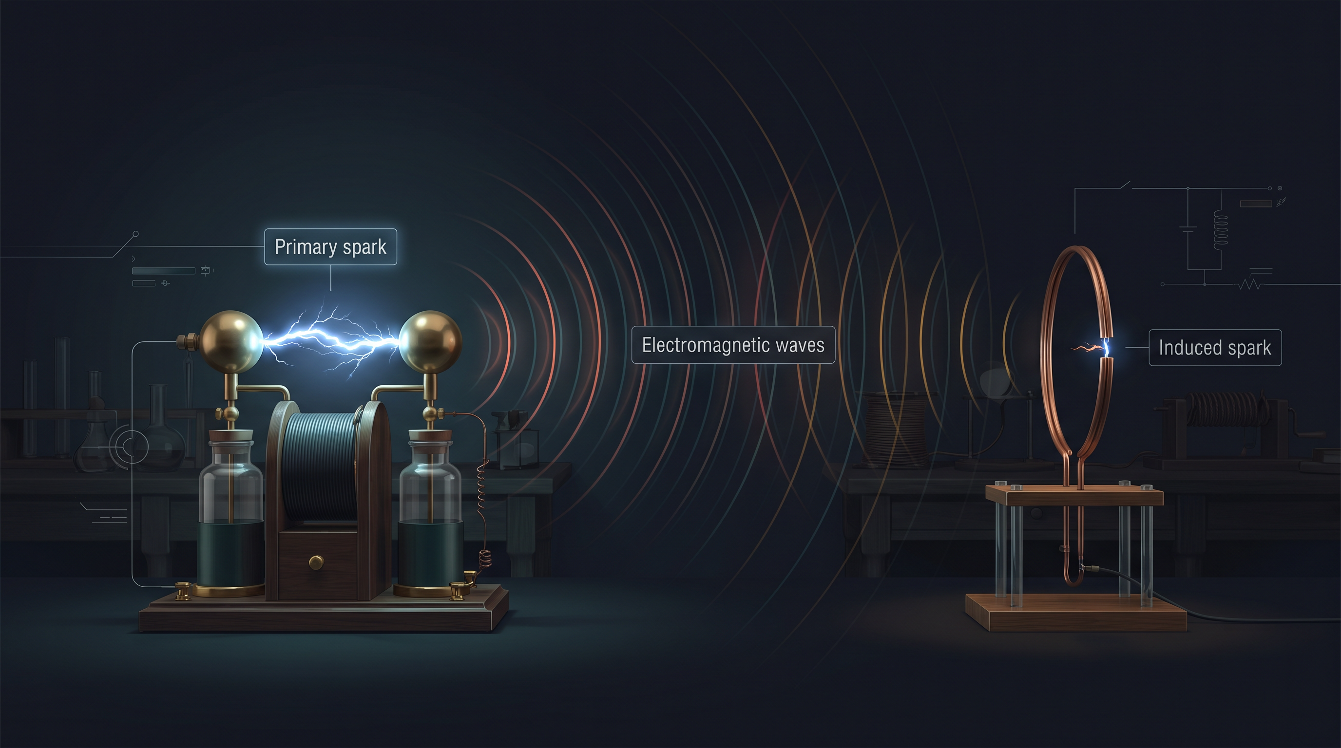
Fig. 8.0 – Hertz’s experimental setup for producing and detecting electromagnetic waves.

NoteCuriosity Corner

Q1. How can a magnetic field appear in a region such as the gap between capacitor plates, where no current of moving charges is actually flowing? Q2. Maxwell calculated the speed of these predicted waves from purely electric and magnetic constants, and it came out equal to the speed of light. What does this coincidence tell us about the nature of light? Q3. In an electromagnetic wave, how are the electric field, the magnetic field, and the direction in which the wave travels arranged relative to one another? Q4. Radio waves, microwaves, visible light, X-rays and gamma rays seem completely different from one another. Are they truly different things, or the same phenomenon in disguise? Q5. Why does a microwave oven heat the water in food so effectively, while radio waves of a different frequency pass through us harmlessly?

By the end of this chapter, you will be able to answer each of these questions.

8.1 Introduction

In Chapter 4 you learnt an important fact linking electricity and magnetism: an electric current produces a magnetic field in the space around it, and because of this, two wires carrying current exert a magnetic force on each other. A magnetic field is a region around a magnet or a current in which a magnetic force can be felt.

Later, in Chapter 6, you saw the reverse effect. A magnetic field that changes with time sets up an electric field. An electric field is a region in which an electric charge experiences a force. This raised a natural and deep question: if a changing magnetic field can create an electric field, can a changing electric field create a magnetic field in return?

James Clerk Maxwell (1831–1879) argued that the answer is yes. According to Maxwell, a magnetic field is produced not only by an electric current, but also by an electric field that is changing with time. This was a bold claim, because until then a magnetic field was thought to come only from moving charges.

Maxwell reached this idea while examining Ampere’s circuital law. This law, studied in Chapter 4, relates the magnetic field along a closed loop to the electric current passing through any surface bounded by that loop. When Maxwell applied it to find the magnetic field near a capacitor connected to a time-varying current, he found a puzzling inconsistency: the law gave different answers depending on which surface was chosen.

To remove this inconsistency, Maxwell proposed the existence of an additional current, which he named the displacement current. This is not a current of moving charges, but an effective current produced by a changing electric field, and it acts as a source of magnetic field just as an ordinary current does.

NoteExam Corner

Q. Why did Maxwell add a new term to a law that already worked well for steady currents?

A. For steady currents in ordinary circuits, Ampere’s law gives correct results. The trouble appears only in situations like a charging capacitor, where a region has a changing electric field but no flowing charges. The extra displacement-current term is what keeps the law consistent in such cases.

Maxwell went further and formulated a complete set of equations connecting electric and magnetic fields to their sources — the electric charges and currents. These are known as Maxwell’s equations. Together with the Lorentz force formula from Chapter 4 (which gives the force on a charge due to electric and magnetic fields), they express all the basic laws of electromagnetism in mathematical form.

The most important prediction to come out of Maxwell’s equations is the existence of electromagnetic waves. An electromagnetic wave is a disturbance made of coupled electric and magnetic fields, both varying with time, that travels through space. Because each field, while changing, keeps generating the other, the pair can sustain itself and move forward even through empty space.

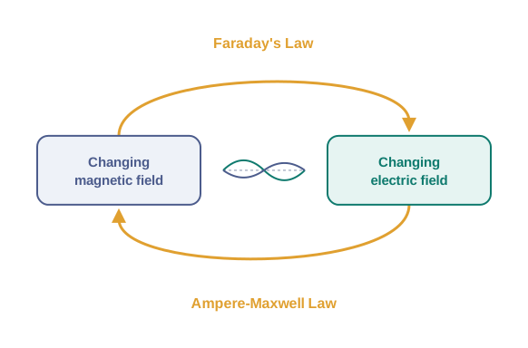
Fig. 8.1a – Mutual regeneration of electric and magnetic fields.

When Maxwell calculated the speed of these predicted waves from the known electric and magnetic constants, the value came out very close to \(3 \\times 10^{8}\) m/s — the speed of light measured in optical experiments. This striking match led to a remarkable conclusion: light itself is an electromagnetic wave. In one stroke, Maxwell’s work united three subjects that had been studied separately — electricity, magnetism, and light.

NoteCuriosity Corner

Q2. Maxwell calculated the speed of these predicted waves from purely electric and magnetic constants, and it came out equal to the speed of light. What does this coincidence tell us about the nature of light?

A. It tells us that light is itself an electromagnetic wave. Maxwell found that his predicted waves travel through vacuum at \(c = 1/\\sqrt{\\mu\_0\\varepsilon\_0}\), a speed fixed entirely by the electric and magnetic constants \(\\varepsilon\_0\) and \(\\mu\_0\) — and this value matched the measured speed of light almost exactly. That agreement was too precise to be a coincidence: it revealed that light is not a separate phenomenon but one member of the family of electromagnetic waves, so optics and electromagnetism are unified.

The prediction was later confirmed by experiment. Hertz, in 1885, demonstrated the existence of electromagnetic waves in the laboratory. Their practical use by Marconi and others soon led to the revolution in long-distance communication that continues to shape the world today.

NoteSide Note

James Clerk Maxwell (1831–1879) was born in Edinburgh, Scotland, and ranks among the greatest physicists of the nineteenth century. Beyond electromagnetism, he studied the behaviour of gases, deriving how the speeds of molecules in a gas are distributed, and was among the first to obtain reliable estimates of molecular quantities such as viscosity. His greatest achievement was gathering the separate discoveries of Coulomb, Oersted, Ampere and Faraday into one consistent set of equations — now called Maxwell’s equations — from which he concluded that light is an electromagnetic wave. Interestingly, Maxwell did not accept the idea, suggested by Faraday’s laws of electrolysis, that electricity is made of particles.

This chapter follows Maxwell’s ideas step by step. We first discuss why the displacement current is needed and what follows from it. We then give a descriptive account of electromagnetic waves. Finally, we survey the broad electromagnetic spectrum — the full family of electromagnetic waves arranged by wavelength — stretching from gamma (\(\\gamma\)) rays, with wavelengths of about \(10^{-12}\) m, all the way to long radio waves, with wavelengths of about \(10^{6}\) m.

8.2 Displacement Current

In Chapter 4 we saw that an electric current sets up a magnetic field around it. Maxwell showed that, for the laws of physics to stay logically consistent, a changing electric field must also set up a magnetic field. This idea is of great importance, because it is exactly what explains the existence of radio waves, gamma rays, visible light, and every other form of electromagnetic wave.

To see how a changing electric field can produce a magnetic field, let us study the charging of a capacitor. Recall from Chapter 2 that a capacitor is a device made of two conductors — here, two parallel metal plates — separated by a gap. While the capacitor is charging, charges flow along the connecting wires and pile up on the plates, but no charge actually crosses the empty gap between the plates. We will apply Ampere’s circuital law, first met in Chapter 4, to this situation.

Ampere’s circuital law, in its original form, relates the magnetic field along a closed loop to the current threading through it:

\[\\oint \\vec{B}\\cdot d\\vec{l} = \\mu\_0, i(t) \\tag{8.1}\]

Here the left side is the line integral of the magnetic field \(\\vec{B}\) (in tesla, T) taken all the way around a chosen closed loop, \(d\\vec{l}\) is a small length element of that loop (in metre, m), \(\\mu\_0\) is the permeability of free space (in T·m·A⁻¹), and \(i(t)\) is the current (in ampere, A) passing through any surface bounded by the loop.

NotePrinciple / Law

Ampere’s circuital law (original form): The line integral of the magnetic field around any closed loop equals \(\\mu\_0\) times the conduction current passing through any surface bounded by that loop.

Now let us use this law to find the magnetic field at a point P lying outside the capacitor, in the region around the connecting wire, as shown in Fig. 8.2(a). We choose a plane circular loop of radius \(r\) whose plane is perpendicular to the wire and which is centred on the wire.

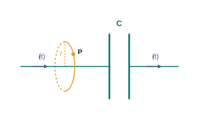
Fig. 8.2(a) – A plane circular loop around the charging wire.

By symmetry, the magnetic field must point along the circumference of this circular loop and must have the same magnitude at every point on it. If \(B\) is this magnitude, the left side of Eq. (8.1) becomes \(B(2\\pi r)\), and so

\[B(2\\pi r) = \\mu\_0, i(t) \\tag{8.2}\]

This gives a definite, non-zero magnetic field at P. So far, so good.

Here is where the trouble begins. The loop is only the boundary; Ampere’s law lets us stretch any surface across it, and the answer should not depend on our choice. Consider a pot-shaped surface, shown in Fig. 8.3(b), whose rim is the same circular loop but whose bottom dips between the capacitor plates. A second option is a surface shaped like a tiffin box without its lid, shown in Fig. 8.4(c), again with the same circular rim but with its flat bottom S lying between the plates.

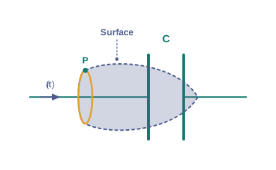
Fig. 8.3(b) – A pot-shaped surface bounded by the same loop.

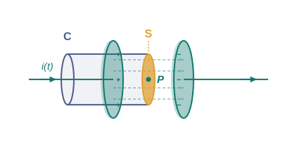
Fig. 8.4(c) – A tiffin-box-shaped surface between the plates.

For these surfaces, the left side of Eq. (8.1) is unchanged, because the loop is the same. But now the right side is different: no charges flow across the gap between the plates, so no conduction current passes through the pot-shaped or tiffin-shaped surfaces. The right side becomes zero, not \(\\mu\_0 i\). We are left with a contradiction: computed one way, there is a magnetic field at P; computed another way, the field at P is zero.

NoteExam Corner

Q. The loop is exactly the same in both cases. Why should the surface we imagine stretched across it change the current we count?

A. Physically, it should not. The magnetic field at P is a real, definite quantity and cannot depend on an imaginary surface we choose. The fact that Ampere’s law gives two different answers is the clue that the law, as first written, is incomplete.

Since the contradiction comes from Ampere’s law itself, the law must be missing something. Whatever the missing term is, it must be built so that we get the same magnetic field at P no matter which surface is used.

We can actually guess the missing term by looking carefully at Fig. 8.4(c). Is there anything at all passing through the surface S between the plates? Yes — the electric field is there. Between the plates of a capacitor of plate area \(A\) carrying total charge \(Q\), the magnitude of the electric field is

\[E = \\frac{Q/A}{\\varepsilon\_0}\]

as established earlier (Eq. 2.41), where \(\\varepsilon\_0\) is the permittivity of free space. This field is perpendicular to the surface S, has the same value over the whole plate area \(A\), and drops to zero outside the plates.

To measure “how much” of this electric field passes through the surface, we use the idea of electric flux. Electric flux \(\\Phi\_E\) through a surface is a measure of the number of electric field lines crossing it; for a uniform field perpendicular to a flat area, it is simply the field magnitude multiplied by that area. Using Gauss’s law, the electric flux through S is

\[\\Phi\_E = |\\vec{E}|,A = \\frac{1}{\\varepsilon\_0}\\frac{Q}{A},A = \\frac{Q}{\\varepsilon\_0} \\tag{8.3}\]

Now, while the capacitor charges, the charge \(Q\) on the plates changes with time, and this changing charge is exactly what the wire current carries: \(i = dQ/dt\). Differentiating Eq. (8.3) with respect to time gives

\[\\frac{d\\Phi\_E}{dt} = \\frac{d}{dt}\\left(\\frac{Q}{\\varepsilon\_0}\\right) = \\frac{1}{\\varepsilon\_0}\\frac{dQ}{dt}\]

This implies that, for consistency,

\[\\varepsilon\_0\\left(\\frac{d\\Phi\_E}{dt}\\right) = i \\tag{8.4}\]

Look at what Eq. (8.4) says. The quantity \(\\varepsilon\_0,(d\\Phi\_E/dt)\), built purely from a changing electric field, comes out exactly equal to the conduction current \(i\) flowing in the wire. This is the missing term.

If we now generalise Ampere’s law by adding, to the conduction current through a surface, this extra term equal to \(\\varepsilon\_0\) times the rate of change of electric flux through the same surface, then the total current comes out the same for every choice of surface. The contradiction disappears. The magnetic field \(B\) at P is now non-zero whichever surface we use, and \(B\) at the outside point P matches \(B\) at a point M just inside the gap, exactly as it should.

The current that flows because of the actual movement of charges through a conductor is called the conduction current. The new term in Eq. (8.4), which arises from a changing electric field (an old name for a changing electric field is “electric displacement”), is called the displacement current, or Maxwell’s displacement current.

NoteDefinition

Conduction current: the current due to the actual flow of charges, such as electrons moving through a conductor.

NoteDefinition

Displacement current (Maxwell’s displacement current): the current-like quantity \(i\_d = \\varepsilon\_0,\\dfrac{d\\Phi\_E}{dt}\) produced by a time-varying electric field. It acts as a source of magnetic field in exactly the same way as a conduction current, even though no charges flow.

This is precisely why a magnetic field exists in the gap between the plates, where not a single charge crosses over: the growing electric field there behaves as a displacement current and produces the field.

NoteCuriosity Corner

Q1. How can a magnetic field appear in a region such as the gap between capacitor plates, where no current of moving charges is actually flowing?

A. Through Maxwell’s displacement current. In the gap no charges cross, but while the capacitor charges the electric field there changes with time, and a changing electric flux acts exactly like a current in producing a magnetic field. Maxwell defined this displacement current as \(i\_d = \\varepsilon\_0\\dfrac{d\\Phi\_E}{dt}\); it equals the conduction current in the wires and continues the current through the gap, so a magnetic field appears there just as it does around the wire, even though no charge moves across.

Figure 8.5 shows the directions of the electric field \(\\vec{E}\) and the magnetic field \(\\vec{B}\) inside the parallel plate capacitor for the case discussed above.

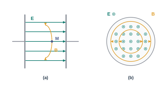
Fig. 8.5(a) – Electric and magnetic fields between the capacitor plates.

Maxwell’s generalisation can now be stated simply: the source of a magnetic field is not just the conduction current due to flowing charges, but also the time rate of change of the electric field. More precisely, the total current \(i\) is the sum of the conduction current \(i\_c\) and the displacement current \(i\_d;(=\\varepsilon\_0, d\\Phi\_E/dt)\):

\[i = i\_c + i\_d = i\_c + \\varepsilon\_0\\frac{d\\Phi\_E}{dt} \\tag{8.5}\]

In plain terms: outside the capacitor plates there is only conduction current, so \(i\_c = i\) and \(i\_d = 0\). Between the plates there is no conduction current, so \(i\_c = 0\) and \(i\_d = i\). The current is therefore never actually broken — what flows in the wire as conduction current continues across the gap as displacement current of the same size.

NoteExam Corner

Q. Inside the capacitor gap, no electrons cross from one plate to the other. Then what “carries” the current across the gap?

A. Nothing material crosses the gap. As charge builds up on the plates, the electric field between them keeps growing, and this changing field acts exactly like a current of the same magnitude. This is why the circuit’s current appears continuous even though the plates are not connected.

NoteNumerical 8.1

While a parallel plate capacitor is being charged, the charge on its plates increases at a steady rate of \(6.0 \\times 10^{-6}\) C s⁻¹. Find (a) the conduction current in the connecting wires and (b) the displacement current in the region between the plates.

The corrected and complete form of Ampere’s law has the same appearance as Eq. (8.1), with one change: the “total current through any surface bounded by the loop” now means the sum of the conduction current and the displacement current. The generalised law is

\[\\oint \\vec{B}\\cdot d\\vec{l} = \\mu\_0, i\_c + \\mu\_0,\\varepsilon\_0\\frac{d\\Phi\_E}{dt} \\tag{8.6}\]

and is known as the Ampere–Maxwell law.

NotePrinciple / Law

Ampere–Maxwell law: The line integral of the magnetic field around a closed loop equals \(\\mu\_0\) times the total current through any surface bounded by that loop, where the total current is the sum of the conduction current \(i\_c\) and the displacement current \(\\varepsilon\_0,d\\Phi\_E/dt\).

In all respects, the displacement current has the same physical effects as the conduction current. In some situations — for example, a steady electric field in a conducting wire — the displacement current is zero, because \(\\vec{E}\) is not changing. In others, such as the charging capacitor, conduction and displacement currents are present in different regions of space. In most real cases the two occur together in the same region, since no medium is a perfect conductor or a perfect insulator. Most striking of all, there can be large regions of space with no conduction current but only a displacement current, due to a time-varying electric field. In such a region we still expect a magnetic field, even though there is no current-carrying source anywhere nearby.

This prediction can be tested. The magnetic field at a point such as M between the plates in Fig. 8.5(a) can actually be measured, and it is found to equal the field just outside at P — direct evidence that the displacement current is real.

The displacement current has, quite literally, far-reaching consequences. The most immediate is that the laws of electricity and magnetism now look far more symmetrical. Recall Faraday’s law of induction from Chapter 6: it states that a changing magnetic flux produces an induced emf. An emf between two points is the work done per unit charge in moving a charge from one point to the other, and the existence of an emf means there is an electric field. So Faraday’s law can be restated as: a magnetic field changing with time gives rise to an electric field. The new result — an electric field changing with time gives rise to a magnetic field — is the exact mirror image, and it is a direct consequence of the displacement current being a source of magnetic field.

Thus, time-varying electric and magnetic fields generate each other. Faraday’s law and the Ampere–Maxwell law together express this mutual generation quantitatively, with the current taken as the total current of Eq. (8.5). One very important consequence of this symmetry is the existence of electromagnetic waves, which we take up in the next section.

NoteSide Note

The symmetry between electricity and magnetism is close but not perfect. A magnetic field has no known “sources” of its own — that is, there are no known magnetic monopoles (isolated north or south poles) that would play the same role for magnetism that electric charges play for electricity.

Maxwell’s Equations in Vacuum

Collected together, the four fundamental equations of electromagnetism in vacuum are:

\[1.\\quad \\oint \\vec{E}\\cdot d\\vec{A} = \\frac{Q}{\\varepsilon\_0} \\qquad \\text{(Gauss's Law for electricity)}\]

\[2.\\quad \\oint \\vec{B}\\cdot d\\vec{A} = 0 \\qquad \\text{(Gauss's Law for magnetism)}\]

\[3.\\quad \\oint \\vec{E}\\cdot d\\vec{l} = -\\frac{d\\Phi\_B}{dt} \\qquad \\text{(Faraday's Law)}\]

\[4.\\quad \\oint \\vec{B}\\cdot d\\vec{l} = \\mu\_0, i\_c + \\mu\_0,\\varepsilon\_0\\frac{d\\Phi\_E}{dt} \\qquad \\text{(Ampere–Maxwell Law)}\]

Here \(\\Phi\_B\) is the magnetic flux through a surface. The first two are Gauss’s laws for the electric and magnetic fields; the third is Faraday’s law of induction; and the fourth is the Ampere–Maxwell law we have just built. Together with the Lorentz force formula, these equations summarise the whole of classical electromagnetism.

8.3 Electromagnetic Waves

8.3.1 Sources of electromagnetic waves

How are electromagnetic waves actually produced? Not by every charge. A charge sitting still produces only a steady electrostatic field, and a charge moving with constant velocity (a steady current) produces a magnetic field that does not change with time. Neither of these can send out an electromagnetic wave.

It is an important result of Maxwell’s theory that accelerated charges radiate electromagnetic waves — that is, a charge whose velocity is changing gives out energy as an electromagnetic wave. The full proof lies beyond this book, but we can understand it with simple, qualitative reasoning.

Consider a charge oscillating back and forth with some frequency. An oscillating charge is constantly changing its velocity, so it is an accelerating charge. As it moves, it produces an oscillating electric field in the space around it. By the Ampere–Maxwell law, this changing electric field produces an oscillating magnetic field. That changing magnetic field, by Faraday’s law, in turn produces an oscillating electric field, and so on.

NoteExam Corner

Q. Why must the charge accelerate? Why can’t a charge moving at constant speed give out a wave?

A. A steadily moving charge produces fields that change smoothly but do not “shake” — nothing oscillates, so there is no self-regenerating disturbance. Only when the charge accelerates do the fields change in a way that keeps feeding a companion field, launching a wave that carries energy away.

In this way the oscillating electric and magnetic fields keep regenerating each other as the disturbance travels outward through space. This mutual regeneration is what allows the wave to propagate without any wire or medium. The frequency of the electromagnetic wave produced is naturally equal to the frequency of oscillation of the charge, and the energy carried away by the wave comes at the expense of the energy of the source — the accelerated charge.

From this it might seem easy to test Maxwell’s claim that light is an electromagnetic wave. We might imagine simply building an alternating-current (ac) circuit whose current oscillates at the frequency of visible light — say, yellow light. Unfortunately, this is not possible. The frequency of yellow light is about \(6 \\times 10^{14}\) Hz, whereas even modern electronic circuits can barely reach about \(10^{11}\) Hz.

This is why the first experimental demonstration of electromagnetic waves had to happen at the much lower frequencies of the radio-wave region, as in Hertz’s experiment of 1887. Hertz generated oscillating currents and detected the waves they radiated, confirming Maxwell’s prediction.

Hertz’s success created a sensation and inspired further work. Two achievements deserve special mention.

NoteReal Incident / Discovery

About seven years after Hertz, Jagadish Chandra Bose, working at Calcutta (now Kolkata), succeeded in producing and observing electromagnetic waves of much shorter wavelength than Hertz — in the range of about 25 mm down to 5 mm. Like Hertz’s, his experiment was carried out within the laboratory, but it pushed the study of these waves into a new, shorter-wavelength region.

NoteReal-World Application

At around the same time, Guglielmo Marconi in Italy built on Hertz’s work and managed to transmit electromagnetic waves over distances of many kilometres. Marconi’s experiments mark the beginning of the entire field of long-distance communication using electromagnetic waves — the ancestor of radio, television, and mobile telephony.

NoteSide Note

Heinrich Rudolf Hertz (1857–1894) was a German physicist, the first person to broadcast and receive radio waves. He produced electromagnetic waves, sent them through space, and measured their wavelength and speed, showing that their vibration, reflection, and refraction behaved just like those of light and heat waves — thereby establishing for the first time that all these are the same kind of wave. He also pioneered the study of electric discharge through gases and discovered the photoelectric effect.

8.3.2 Nature of electromagnetic waves

It can be shown from Maxwell’s equations that, in an electromagnetic wave, the electric field and the magnetic field are perpendicular to each other, and both are perpendicular to the direction in which the wave travels. This should feel reasonable from our study of the displacement current.

Look again at the capacitor of Fig. 8.5. The electric field between the plates points straight across, perpendicular to the plates. The magnetic field that this changing electric field creates, through the displacement current, runs along the perimeter of a circle lying in a plane parallel to the plates. So in this case \(\\vec{B}\) and \(\\vec{E}\) are at right angles to each other — and this turns out to be a general feature of electromagnetic waves.

NoteCuriosity Corner

Q3. In an electromagnetic wave, how are the electric field, the magnetic field, and the direction in which the wave travels arranged relative to one another?

A. They are mutually perpendicular. The electric field \(\\vec{E}\) and the magnetic field \(\\vec{B}\) oscillate at right angles to each other, and both are perpendicular to the direction in which the wave travels — so an electromagnetic wave is a transverse wave. The two fields oscillate in step (in phase), and the direction of propagation is along \(\\vec{E}\\times\\vec{B}\); their amplitudes are linked by \(E\_0 = cB\_0\).

Figure 8.6 shows a typical example of a plane electromagnetic wave — a wave whose fields are uniform over any plane perpendicular to the direction of travel — moving along the \(z\) direction. The fields are drawn as they vary with the \(z\) coordinate at one instant of time \(t\).

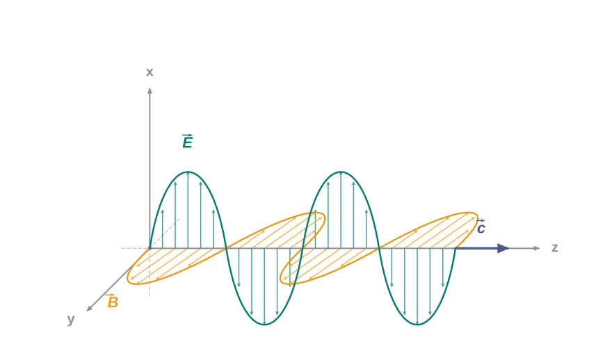
Fig. 8.6 – A plane electromagnetic wave travelling along the z-direction.

In this wave, the electric field \(E\_x\) points along the \(x\)-axis and varies sinusoidally with \(z\), while the magnetic field \(B\_y\) points along the \(y\)-axis and also varies sinusoidally with \(z\). Both fields are perpendicular to each other and to the \(z\) direction of travel. We can write them as

\[E\_x = E\_0 \\sin(kz - \\omega t) \\tag{8.7(a)}\]

\[B\_y = B\_0 \\sin(kz - \\omega t) \\tag{8.7(b)}\]

Here \(E\_0\) and \(B\_0\) are the amplitudes (maximum values) of the electric and magnetic fields, in V·m⁻¹ and tesla (T) respectively. The quantity \(k\) is related to the wavelength \(\\lambda\) (the distance over which the wave pattern repeats, in metre) by

\[k = \\frac{2\\pi}{\\lambda} \\tag{8.8}\]

and \(\\omega\) is the angular frequency (in rad·s⁻¹), which measures how fast the field oscillates in time. The symbol \(k\) is the magnitude of the wave vector (or propagation vector) \(\\vec{k}\), whose direction gives the direction in which the wave travels. From the standard description of a travelling wave, the speed of propagation is \(\\omega/k\).

Putting the field expressions of Eqs. 8.7(a) and 8.7(b) into Maxwell’s equations, one finds

\[\\omega = ck, \\qquad \\text{where } c = \\frac{1}{\\sqrt{\\mu\_0 \\varepsilon\_0}} \\tag{8.9(a)}\]

The relation \(\\omega = ck\) is the usual relation between angular frequency and wave number for any wave (as met in Section 14.4 of the Class XI textbook). It can be rewritten using frequency \(\\nu;(=\\omega/2\\pi)\) and wavelength \(\\lambda;(=2\\pi/k)\) as

\[2\\pi\\nu = c\\left(\\frac{2\\pi}{\\lambda}\\right) \\quad \\text{or} \\quad \\nu\\lambda = c \\tag{8.9(b)}\]

This is the familiar wave relation: frequency times wavelength equals the wave’s speed.

NoteNumerical 8.2

A radio station broadcasts an electromagnetic wave of frequency \(100\) MHz in free space. Taking \(c = 3 \\times 10^{8}\) m s⁻¹, find the wavelength of the wave.

Maxwell’s equations also fix a simple link between the amplitudes of the two fields in the wave:

\[B\_0 = \\frac{E\_0}{c} \\tag{8.10}\]

Because \(c\) is very large, \(B\_0\) comes out numerically much smaller than \(E\_0\) — but this does not mean the magnetic part is unimportant; the two fields carry equal shares of the wave’s energy.

NoteExam Corner

Q. If \(B\_0 = E\_0/c\) makes \(B\_0\) a tiny number, is the magnetic field of light almost negligible?

A. No. The small number is only because of the units and the large value of \(c\). In terms of the physics, the electric and magnetic fields are exactly balanced partners — each regenerates the other, and each carries half the energy of the wave.

We can now note some key features of electromagnetic waves. They are self-sustaining oscillations of electric and magnetic fields — once launched, the two fields keep each other going. They differ from every other wave studied so far, such as sound or waves on a string, in one crucial way: no material medium is needed for the fields to vibrate. Electromagnetic waves travel even through vacuum.

But what happens when a material medium is present? Light, an electromagnetic wave, certainly passes through glass. Inside a medium, the electric and magnetic fields are described using the medium’s permittivity \(\\varepsilon\) and magnetic permeability \(\\mu\) — quantities that measure how the medium modifies electric and magnetic fields compared with empty space. These replace the free-space constants \(\\varepsilon\_0\) and \(\\mu\_0\) in Maxwell’s equations, so that in a medium of permittivity \(\\varepsilon\) and permeability \(\\mu\) the speed of light becomes

\[v = \\frac{1}{\\sqrt{\\mu\\varepsilon}} \\tag{8.11}\]

Thus the speed of light in a substance depends on the electric and magnetic properties of that substance. In the next chapter we will see that the refractive index of one medium relative to another — a measure of how much light bends when passing between them — equals the ratio of the light speeds in the two media.

NoteNumerical 8.3

A transparent medium has permittivity \(\\varepsilon = 4\\varepsilon\_0\) and permeability \(\\mu = \\mu\_0\). Using Eq. (8.11), find the speed of light in this medium in terms of the free-space speed \(c\).

The speed of electromagnetic waves in vacuum is one of the most important constants in physics. Experiments with electromagnetic waves of many different wavelengths show that this speed is the same for all of them — independent of wavelength — to within a few metres per second, at a value of \(3 \\times 10^{8}\) m/s. This constancy is so firmly established, and the value so precisely known, that the speed of light is now used to define the standard of length, the metre.

Finally, the great technological importance of electromagnetic waves comes from their ability to carry energy from one place to another. Radio and television signals from broadcasting stations carry energy across long distances, and light carries energy from the Sun to the Earth — the energy that makes life on Earth possible.

NoteExample 8.1

A plane electromagnetic wave of frequency 25 MHz travels through free space along the x-direction. At a particular point in space and time, the electric field is \(\\vec{E} = 6.3,\\hat{j}\) V/m. Find the magnetic field \(\\vec{B}\) at this point.

Solution: We first find the magnitude of \(\\vec{B}\) using the amplitude relation of Eq. (8.10), which links the electric and magnetic field magnitudes through the speed of light:

\[B = \\frac{E}{c} = \\frac{6.3\\ \\text{V/m}}{3 \\times 10^{8}\\ \\text{m/s}} = 2.1 \\times 10^{-8}\\ \\text{T}\]

To find the direction, note that \(\\vec{E}\) is along the \(y\)-direction and the wave travels along the \(x\)-axis. So \(\\vec{B}\) must be perpendicular to both the \(x\)- and \(y\)-axes. The rule is that \(\\vec{E} \\times \\vec{B}\) points along the direction of propagation, here the \(x\)-direction. Since \((+\\hat{j}) \\times (+\\hat{k}) = \\hat{i}\), the field \(\\vec{B}\) must lie along the \(z\)-direction. Therefore

\[\\vec{B} = 2.1 \\times 10^{-8},\\hat{k}\\ \\text{T}\]

NoteExample 8.2

The magnetic field in a plane electromagnetic wave is given by \(B\_y = (2 \\times 10^{-7})\\ \\text{T}\\ \\sin(0.5 \\times 10^{3},x + 1.5 \\times 10^{11},t)\). (a) Find the wavelength and frequency of the wave. (b) Write an expression for the electric field.

Solution:

1. We compare the given equation with the standard travelling-wave form

\[B\_y = B\_0 \\sin\\left\[2\\pi\\left(\\frac{x}{\\lambda} + \\frac{t}{T}\\right)\\right]\]

Matching the coefficient of \(x\) gives the wavelength, and matching the coefficient of \(t\) gives the frequency:

\[\\lambda = \\frac{2\\pi}{0.5 \\times 10^{3}}\\ \\text{m} = 1.26\\ \\text{cm}\]

\[\\frac{1}{T} = \\nu = \\frac{1.5 \\times 10^{11}}{2\\pi} = 23.9\\ \\text{GHz}\]

2. The amplitude of the electric field follows from Eq. (8.10), \(E\_0 = B\_0 c\):

\[E\_0 = B\_0 c = 2 \\times 10^{-7}\\ \\text{T} \\times 3 \\times 10^{8}\\ \\text{m/s} = 6 \\times 10^{1}\\ \\text{V/m}\]

The electric field must be perpendicular both to the direction of propagation and to the magnetic field. Here \(B\_y\) is along the \(y\)-axis and the wave travels along \(x\), so the electric field lies along the \(z\)-axis:

\[E\_z = 60 \\sin(0.5 \\times 10^{3},x + 1.5 \\times 10^{11},t)\\ \\text{V/m}\]

8.4 Electromagnetic Spectrum

When Maxwell first predicted electromagnetic waves, the only ones known were the visible light waves. The existence of ultraviolet and infrared waves was barely established, and only by the end of the nineteenth century were X-rays and gamma rays discovered. Today we know that electromagnetic waves form a whole family: visible light, X-rays, gamma rays, radio waves, microwaves, ultraviolet and infrared waves.

The arrangement of all these waves according to their frequency (or, equivalently, their wavelength) is called the electromagnetic spectrum, shown in Fig. 8.7. Importantly, there is no sharp dividing line between one kind of wave and the next; the names simply mark rough regions, and neighbouring regions overlap. The classification is based mainly on how the waves are produced and how they are detected — not on any real difference in their basic nature.

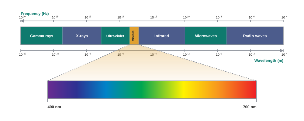
Fig. 8.7 – The electromagnetic spectrum.

This is the key point: radio waves, microwaves, light, X-rays and gamma rays are not different things. They are all electromagnetic waves — the same coupled, self-sustaining oscillation of electric and magnetic fields — differing only in frequency and wavelength. Because all of them travel through vacuum at the same speed \(c\), and because \(\\nu\\lambda = c\), a higher frequency simply means a shorter wavelength. What makes each region behave so differently is how it is produced and how it interacts with matter, both of which depend on frequency.

NoteCuriosity Corner

Q4. Radio waves, microwaves, visible light, X-rays and gamma rays seem completely different from one another. Are they truly different things, or the same phenomenon in disguise?

A. They are the same phenomenon — all are electromagnetic waves, differing only in wavelength (or frequency). Together they form the electromagnetic spectrum, and every one of them travels through vacuum at the same speed \(c\). What makes them seem so different is that their differing frequencies cause them to interact with matter in very different ways — which is why radio waves, light, and X-rays are produced, detected, and used so differently — but their underlying nature is identical.

NoteNumerical 8.4

An X-ray has a wavelength of \(1\\ \\text{nm} = 1 \\times 10^{-9}\) m. Taking \(c = 3 \\times 10^{8}\) m s⁻¹ and using \(\\nu\\lambda = c\), find its frequency and confirm which region of the spectrum it belongs to.

We now describe the different types of electromagnetic waves, going in order of decreasing wavelength — from the longest (radio) to the shortest (gamma).

8.4.1 Radio waves

Radio waves are produced by the accelerated motion of charges in conducting wires, such as the oscillating currents in an antenna. They are the waves used in radio and television communication systems.

Radio waves generally lie in the frequency range from about 500 kHz to about 1000 MHz. Within this, the AM (amplitude modulated) band runs from 530 kHz to 1710 kHz. Higher frequencies, up to 54 MHz, are used for short-wave bands. Television waves occupy the range from 54 MHz to 890 MHz, while the FM (frequency modulated) radio band extends from 88 MHz to 108 MHz.

Cellular phones use radio waves to carry voice communication in the ultrahigh frequency (UHF) band. The details of how such waves are transmitted and received are taken up in Chapter 15.

8.4.2 Microwaves

Microwaves are short-wavelength radio waves, with frequencies in the gigahertz (GHz) range. They are produced by special vacuum tubes called klystrons, magnetrons and Gunn diodes.

Because of their short wavelengths, microwaves are well suited to radar systems used in aircraft navigation. Radar also underlies the speed guns used to measure the speed of fast-moving objects such as cricket balls, tennis serves, and automobiles.

NoteReal-World Application

A speed gun works by sending out microwaves that reflect off a moving object and return with a slightly shifted frequency. From the size of this frequency shift, the instrument calculates the object’s speed — the same radar principle that lets air-traffic controllers track aircraft.

A familiar domestic use is the microwave oven. Here the frequency of the microwaves is deliberately chosen to match the resonant frequency of water molecules. Resonance means that when the driving frequency of a wave matches a natural frequency of a system, energy is transferred to that system most efficiently. Because the microwaves are tuned to water’s resonant frequency, energy passes very efficiently into the kinetic energy of the water molecules, raising the temperature of any food containing water.

This also settles a puzzle: a radio wave of a very different frequency does not match water’s resonance, so it passes through with little energy transfer, while microwaves at the tuned frequency heat the water strongly.

NoteCuriosity Corner

Q5. Why does a microwave oven heat the water in food so effectively, while radio waves of a different frequency pass through us harmlessly?

A. Because a microwave oven is tuned to a frequency that matches the natural response of water molecules. Its microwaves are chosen so that they are efficiently absorbed by the water in food, setting the water molecules into vigorous motion and heating the food from within. Radio waves have a much lower frequency that is not absorbed this way, so they carry little energy per photon and simply pass through us without depositing significant heat — the effect depends strongly on the frequency of the radiation.

8.4.3 Infrared waves

Infrared waves are produced by hot bodies and molecules. This band lies just beyond the low-frequency, long-wavelength (red) end of the visible spectrum.

Infrared waves are often called heat waves. The reason is that water molecules — present in most materials — readily absorb infrared radiation (many other molecules, such as carbon dioxide, CO₂, and ammonia, NH₃, also absorb it). Once absorbed, the energy increases the thermal motion of the molecules; that is, the material heats up and warms its surroundings. Infrared lamps make use of this effect and are used in physical therapy.

Infrared radiation also helps keep the Earth warm through the greenhouse effect. Incoming visible sunlight passes fairly easily through the atmosphere and is absorbed by the Earth’s surface. The warmed surface then re-radiates this energy as infrared (longer wavelength) radiation, which is trapped by greenhouse gases such as carbon dioxide and water vapour, keeping the surface warmer than it would otherwise be.

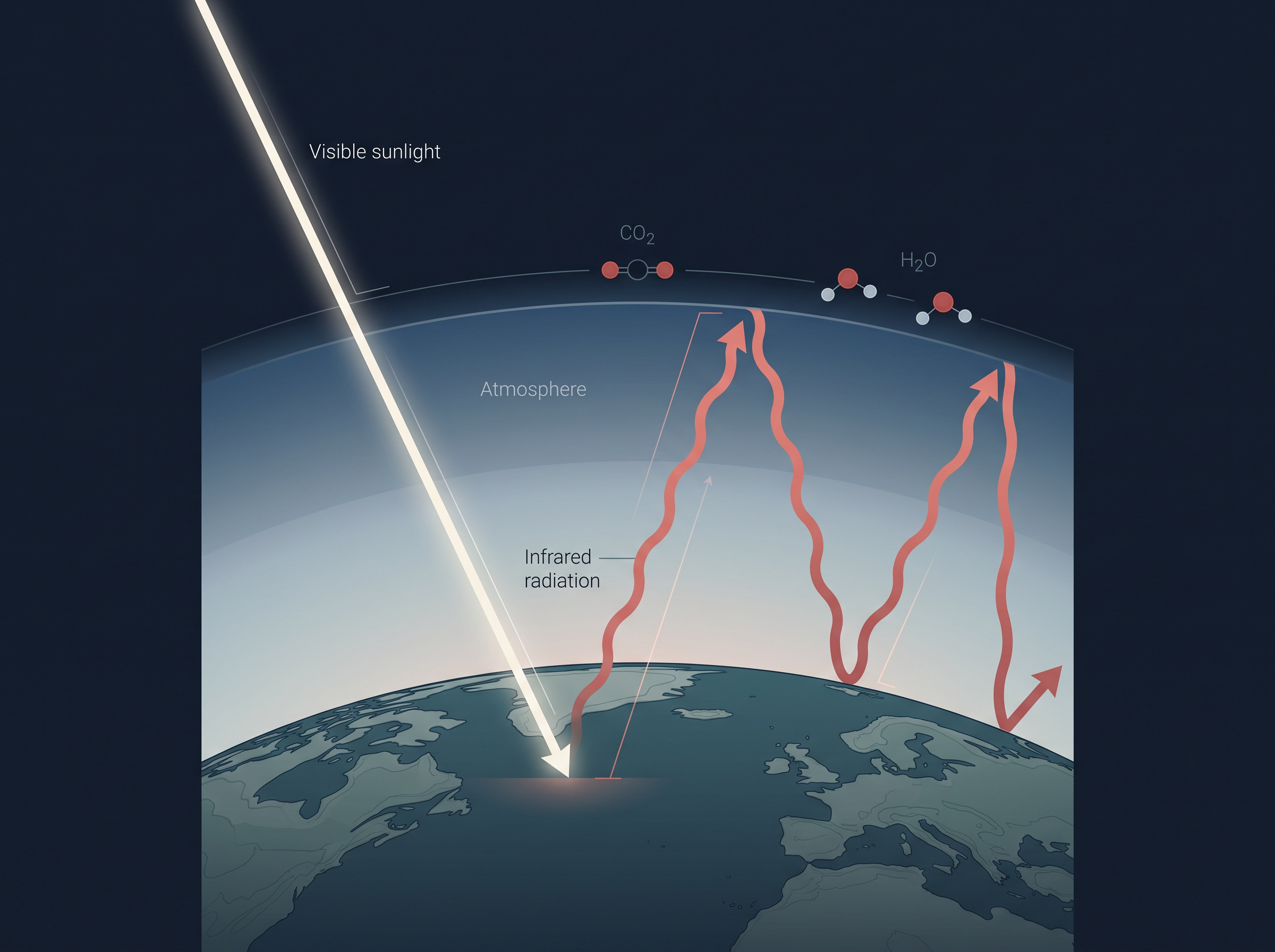
Fig. 8.8a – The greenhouse effect.

Infrared detectors are carried on Earth satellites, both for military purposes and to observe the growth of crops. Everyday electronic devices, such as semiconductor light-emitting diodes (LEDs), also emit infrared.

NoteReal-World Application

The remote controls of televisions, video players and hi-fi systems work by emitting coded pulses of infrared light. The device’s sensor detects these invisible infrared pulses and interprets them as commands, which is why a remote must usually be pointed roughly toward the appliance.

8.4.4 Visible rays

Visible light is the most familiar form of electromagnetic wave — it is the part of the spectrum that the human eye can detect.

It runs from about \(4 \\times 10^{14}\) Hz to about \(7 \\times 10^{14}\) Hz, corresponding to a wavelength range of roughly 700 nm down to 400 nm. Visible light emitted or reflected from the objects around us gives us most of our information about the world, and our eyes have evolved to be sensitive to exactly this range.

Different animals, however, are sensitive to different ranges. For example, snakes can detect infrared waves, and the “visible” range of many insects extends well into the ultraviolet — so these creatures effectively see parts of the spectrum that we cannot.

8.4.5 Ultraviolet rays

Ultraviolet (UV) rays cover wavelengths from about \(4 \\times 10^{-7}\) m (400 nm) down to about \(6 \\times 10^{-10}\) m (0.6 nm). They are produced by special lamps and by very hot bodies. The Sun is an important source of ultraviolet light.

Fortunately, most of the Sun’s UV is absorbed by the ozone layer in the atmosphere, at an altitude of about 40–50 km. This matters because large amounts of UV are harmful to humans. Exposure to UV triggers the skin to produce more melanin — the pigment that darkens skin — causing tanning. Ordinary glass absorbs UV, which is why one cannot get tanned or sunburnt through a glass window.

Because welding arcs give off large amounts of UV, welders wear special glass goggles or face masks to protect their eyes. Owing to their short wavelengths, UV rays can be focused into very narrow beams, useful for high-precision applications.

NoteReal-World Application

Two important uses of ultraviolet light are LASIK (Laser-assisted in situ keratomileusis) eye surgery, where a finely focused UV beam reshapes the cornea to correct vision, and UV lamps in water purifiers, where the radiation kills germs in the water.

The ozone layer’s protective role is so important that its depletion by chlorofluorocarbon (CFC) gases, such as freon, is a matter of serious international concern.

8.4.6 X-rays

Beyond the ultraviolet region lies the X-ray region. We are most familiar with X-rays through their medical uses. They cover wavelengths from about \(10^{-8}\) m (10 nm) down to about \(10^{-13}\) m (\(10^{-4}\) nm).

One common way to generate X-rays is to bombard a metal target with high-energy electrons. X-rays are used both as a diagnostic tool in medicine — for example, to image bones — and as a treatment for certain forms of cancer.

However, because X-rays can damage or destroy living tissues and organisms, great care must be taken to avoid unnecessary or excessive exposure. This is why protective shielding is used during medical X-ray procedures.

8.4.7 Gamma rays

Gamma rays lie in the highest-frequency region of the electromagnetic spectrum, with wavelengths from about \(10^{-10}\) m down to less than \(10^{-14}\) m.

This very high-frequency radiation is produced in nuclear reactions and is also emitted by radioactive nuclei. In medicine, gamma rays are used to destroy cancer cells.

Summary Table

Table 8.1 summarises the different types of electromagnetic waves, together with how each is produced and detected. As noted, the boundaries between regions are not sharp, and neighbouring regions overlap.

Table 8.1 — Different types of electromagnetic waves

Type	Wavelength range	Production	Detection
Radio	\(> 0.1\) m	Rapid acceleration and deceleration of electrons in aerials	Receiver’s aerials
Microwave	0.1 m to 1 mm	Klystron valve or magnetron valve	Point contact diodes
Infra-red	1 mm to 700 nm	Vibration of atoms and molecules	Thermopiles; Bolometer; Infrared photographic film
Light	700 nm to 400 nm	Electrons in atoms emit light when they move from one energy level to a lower energy level	The eye; Photocells; Photographic film
Ultraviolet	400 nm to 1 nm	Inner shell electrons in atoms moving from one energy level to a lower level	Photocells; Photographic film
X-rays	1 nm to \(10^{-3}\) nm	X-ray tubes or inner shell electrons	Photographic film; Geiger tubes; Ionisation chamber
Gamma rays	\(< 10^{-3}\) nm	Radioactive decay of the nucleus	Photographic film; Geiger tubes; Ionisation chamber

Notice how, moving down the table, the production mechanism shifts from the gross acceleration of electrons in wires (radio), to the vibration of atoms and molecules (infrared), to jumps of electrons between energy levels in atoms (visible, ultraviolet, X-rays), and finally to processes inside the atomic nucleus (gamma rays). The higher the frequency of the radiation, the deeper inside matter its source tends to lie.

8.5 Summary

1. Maxwell found an inconsistency in Ampere’s law and, to remove it, proposed an additional current called the displacement current. This current arises from a time-varying electric field and is given by \[i\_d = \\varepsilon\_0 \\frac{d\\Phi\_E}{dt}\] It acts as a source of magnetic field in exactly the same way as an ordinary conduction current.
2. An accelerating charge produces electromagnetic waves. A charge oscillating harmonically with frequency \(\\nu\) produces electromagnetic waves of the same frequency \(\\nu\). An oscillating electric dipole is therefore a basic source of electromagnetic waves.
3. Electromagnetic waves with wavelengths of the order of a few metres were first produced and detected in the laboratory by Hertz in 1887. This verified a basic prediction of Maxwell’s equations.
4. In an electromagnetic wave, the electric and magnetic fields oscillate sinusoidally in both space and time. The oscillating fields \(\\vec{E}\) and \(\\vec{B}\) are perpendicular to each other, and both are perpendicular to the direction in which the wave travels. For a wave of frequency \(\\nu\) and wavelength \(\\lambda\) propagating along the \(z\)-direction, \[E = E\_x(t) = E\_0 \\sin(kz - \\omega t) = E\_0 \\sin\\left\[2\\pi\\left(\\frac{z}{\\lambda} - \\nu t\\right)\\right] = E\_0 \\sin\\left\[2\\pi\\left(\\frac{z}{\\lambda} - \\frac{t}{T}\\right)\\right]\] \[B = B\_y(t) = B\_0 \\sin(kz - \\omega t) = B\_0 \\sin\\left\[2\\pi\\left(\\frac{z}{\\lambda} - \\nu t\\right)\\right] = B\_0 \\sin\\left\[2\\pi\\left(\\frac{z}{\\lambda} - \\frac{t}{T}\\right)\\right]\] The amplitudes of the two fields are related by \(E\_0/B\_0 = c\).
5. The speed \(c\) of an electromagnetic wave in vacuum is fixed by the free-space permeability \(\\mu\_0\) and permittivity \(\\varepsilon\_0\): \[c = \\frac{1}{\\sqrt{\\mu\_0 \\varepsilon\_0}}\] This value equals the speed of light measured in optical experiments. Hence light is an electromagnetic wave, and \(c\) is also the speed of light. All other electromagnetic waves travel with this same speed \(c\) in free space. In a material medium of permeability \(\\mu\) and permittivity \(\\varepsilon\), the speed of light (or of any electromagnetic wave) becomes \[v = \\frac{1}{\\sqrt{\\mu\\varepsilon}}\]
6. The spectrum of electromagnetic waves stretches, in principle, over an infinite range of wavelengths. Its different regions are known by different names — \(\\gamma\)-rays, X-rays, ultraviolet rays, visible rays, infrared rays, microwaves and radio waves — listed here in order of increasing wavelength, from about \(10^{-2}\) Å (or \(10^{-12}\) m) up to about \(10^{6}\) m. These waves interact with matter through their electric and magnetic fields, which set the charges present in all matter into oscillation. The detailed way in which a wave is absorbed, scattered, and so on depends both on its wavelength and on the nature of the atoms and molecules in the medium.

8.6 Points to Ponder

1. The basic difference between the various types of electromagnetic waves lies only in their wavelength or frequency — since all of them travel through vacuum at the very same speed \(c\). It is precisely because their frequencies differ that they differ so greatly in the way they interact with matter.
2. Accelerated charged particles radiate electromagnetic waves, and the wavelength of the wave is often related to the characteristic size of the system that produces it. For example, gamma radiation, with wavelengths of about \(10^{-14}\) m to \(10^{-15}\) m, typically comes from an atomic nucleus. X-rays are emitted from heavy atoms, while radio waves are produced by electrons accelerating in a circuit. A transmitting antenna radiates most efficiently when its length is about equal to the wavelength it sends out. Interestingly, the visible light emitted by atoms has a wavelength much larger than the size of an atom itself.
3. Infrared waves have frequencies lower than those of visible light. Because of this, they set into vibration not just the electrons but entire atoms or molecules of a substance. This vibration raises the internal energy, and therefore the temperature, of the substance — which is exactly why infrared waves are commonly called heat waves.
4. The centre of the sensitivity of our eyes coincides with the centre of the wavelength distribution of sunlight. This is no accident: human vision has evolved to be most sensitive to the wavelengths that arrive most strongly from the Sun.

8.7 NCERT Questions

1. Figure 8.9 shows a capacitor made of two circular plates each of radius 12 cm, and separated by 5.0 cm. The capacitor is being charged by an external source (not shown in the figure). The charging current is constant and equal to 0.15 A.

1. Calculate the capacitance and the rate of change of potential difference between the plates.
2. Obtain the displacement current across the plates.
3. Is Kirchhoff’s first rule (junction rule) valid at each plate of the capacitor? Explain.

2. A parallel plate capacitor (Fig. 8.10) made of circular plates each of radius \(R = 6.0\) cm has a capacitance \(C = 100\) pF. The capacitor is connected to a 230 V ac supply with a (angular) frequency of 300 rad s⁻¹.

1. What is the rms value of the conduction current?
2. Is the conduction current equal to the displacement current?
3. Determine the amplitude of \(B\) at a point 3.0 cm from the axis between the plates.

3. What physical quantity is the same for X-rays of wavelength \(10^{-10}\) m, red light of wavelength 6800 Å and radiowaves of wavelength 500 m?
4. A plane electromagnetic wave travels in vacuum along the \(z\)-direction. What can you say about the directions of its electric and magnetic field vectors? If the frequency of the wave is 30 MHz, what is its wavelength?
5. A radio can tune in to any station in the 7.5 MHz to 12 MHz band. What is the corresponding wavelength band?
6. A charged particle oscillates about its mean equilibrium position with a frequency of \(10^{9}\) Hz. What is the frequency of the electromagnetic waves produced by the oscillator?
7. The amplitude of the magnetic field part of a harmonic electromagnetic wave in vacuum is \(B\_0 = 510\) nT. What is the amplitude of the electric field part of the wave?
8. Suppose that the electric field amplitude of an electromagnetic wave is \(E\_0 = 120\) N/C and that its frequency is \(\\nu = 50.0\) MHz.

1. Determine \(B\_0\), \(\\omega\), \(k\), and \(\\lambda\).
2. Find expressions for \(\\vec{E}\) and \(\\vec{B}\).

9. The terminology of different parts of the electromagnetic spectrum is given in the text. Use the formula \(E = h\\nu\) (for the energy of a quantum of radiation: photon) and obtain the photon energy in units of eV for different parts of the electromagnetic spectrum. In what way are the different scales of photon energies that you obtain related to the sources of electromagnetic radiation?
10. In a plane electromagnetic wave, the electric field oscillates sinusoidally at a frequency of \(2.0 \\times 10^{10}\) Hz and amplitude 48 V m⁻¹.

1. What is the wavelength of the wave?
2. What is the amplitude of the oscillating magnetic field?
3. Show that the average energy density of the \(\\vec{E}\) field equals the average energy density of the \(\\vec{B}\) field. [\(c = 3 \\times 10^{8}\) m s⁻¹.]

8.8 Check Your Concepts

1. When Ampere’s circuital law in its original form is applied to a charging capacitor, it gives two different answers for the magnetic field depending on the surface chosen. Explain why this contradiction arises, and describe how the introduction of the displacement current resolves it.
2. A student argues: “Since no charge actually crosses the gap between the plates of a charging capacitor, there can be no magnetic field in that region.” State whether this reasoning is correct and justify your answer using the idea of displacement current.
3. Why can a charge moving with constant velocity not act as a source of electromagnetic waves, whereas a charge oscillating about a mean position can? Explain in terms of the fields the charge produces.
4. The amplitude relation \(B\_0 = E\_0/c\) makes the numerical value of \(B\_0\) very small compared with \(E\_0\). Does this mean that the magnetic field carries much less of the wave’s energy than the electric field? Explain your reasoning.
5. Explain why the first experimental demonstration of electromagnetic waves had to be carried out in the radio-frequency region, rather than at the frequency of visible light.
6. You cannot get a suntan while sitting indoors behind a closed glass window, even in strong sunlight. Identify the type of radiation responsible for tanning and use its interaction with glass to explain this observation.

8.9 Practice with Numericals

1. A parallel plate capacitor of capacitance 20 pF is being charged so that the potential difference across its plates increases at a steady rate of \(5.0 \\times 10^{4}\) V s⁻¹. Find the displacement current between the plates.
2. The electric field amplitude of a plane electromagnetic wave travelling in vacuum is \(E\_0 = 6.0\) N C⁻¹. Taking \(c = 3 \\times 10^{8}\) m s⁻¹, find the amplitude \(B\_0\) of its magnetic field.
3. An FM radio station transmits at a frequency of 90 MHz. Using \(\\nu\\lambda = c\) with \(c = 3 \\times 10^{8}\) m s⁻¹, find the wavelength of the broadcast wave.
4. Light of wavelength 500 nm travels through vacuum. Taking \(c = 3 \\times 10^{8}\) m s⁻¹, find its frequency and state which region of the electromagnetic spectrum it belongs to.
5. The electric field of a plane electromagnetic wave in vacuum is given by \(E\_x = 24 \\sin(\\omega t - kz)\) V m⁻¹, where \(\\omega = 6.0 \\times 10^{9}\) rad s⁻¹. Taking \(c = 3 \\times 10^{8}\) m s⁻¹, find (a) the wave number \(k\), (b) the wavelength \(\\lambda\), (c) the frequency \(\\nu\), and (d) the amplitude \(B\_0\) of the magnetic field.
6. A transparent medium has permittivity \(\\varepsilon = 9\\varepsilon\_0\) and permeability \(\\mu = \\mu\_0\). Using \(v = 1/\\sqrt{\\mu\\varepsilon}\) and \(c = 3 \\times 10^{8}\) m s⁻¹, find the speed of an electromagnetic wave in this medium.