Every month, price collectors visit a fixed list of shops in selected towns and villages and write down the price of the same set of items — a kilogram of rice, a litre of kerosene, a school shirt. Those thousands of separate figures are checked, grouped and averaged, and end up as a single index of consumer prices that tells the country how fast the cost of living is rising.
Nothing in that exercise happens by itself. Figures have to be obtained from somebody, by some method, at some cost in money, time and effort, and no inquiry can afford to observe everything it might like to. Once obtained, a mass of figures lying in no particular order tells nobody anything, so it has to be organised — grouped, counted and arranged into a series. Only then can it be set out in a table, a diagram or a graph in which a reader can see the pattern at a glance.
This chapter takes those three stages in order: where figures come from and how they are collected, how raw figures are classified into statistical series, and how organised figures are finally presented.
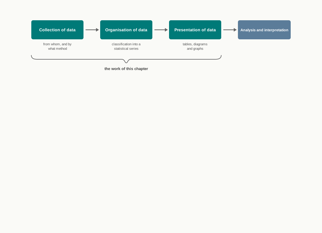
17.1 Data and the Statistical Inquiry
Statistics works on figures. Before an average can be found, a price index built or a correlation measured, somebody must go out and obtain the figures — from households, from factories, from shops or from records already lying in an office. That first step decides everything that follows, because a conclusion can never be more reliable than the figures it rests on.
Obtaining figures is itself an act of choice under constraint. An investigation has limited money, limited time and limited people, so it cannot record everything about everybody. It must decide what exactly to measure, over what area, over what period, and from whom. This section explains what data are and how an organised inquiry sets about collecting them.
17.1.1 Meaning of Data
Data are numerical descriptions of facts relating to some group of people, objects or events. If the ages of all the students in a class are noted down, the whole set of those figures is data. So are the incomes of a set of families, the marks obtained by a batch of candidates, or the annual production of rice in India over a run of years.
Data Data are numerical descriptions of certain observations or things, collected in respect of a group of persons, objects or events relating to a particular inquiry.
A single figure on its own is rarely of interest. Data become useful only as a set, because it is the set that shows how large the items are, how they differ from one another and how they are moving over time.
Data are the raw figures themselves. Information is what emerges after those figures have been organised and interpreted. The same data may yield different information depending on how they are treated.
17.1.2 Raw Data and Ordered Data
Figures as first written down are in no particular order. If the height of fifty students is recorded roll number by roll number, the resulting list follows the roll register and nothing else. Such a mass of unarranged figures is called raw data.
Raw Data Raw data are collected data that have not been organised numerically. They are a mass of figures in their original, crude form, arranged in no order of magnitude.
The first thing a statistician does with raw data is to arrange them in order of size — smallest first or largest first. Figures so arranged are called ordered data, and the arrangement itself is an array. Table 17.1 shows the same ten marks in both forms.
Table 17.1 — Marks Of Ten Students In Raw Form And As An Ordered Array | Roll number | Marks as recorded (raw data) | Marks in ascending order (ordered data) | |—|—|—| | 1 | 12 | 12 | | 2 | 19 | 19 | | 3 | 46 | 27 | | 4 | 36 | 35 | | 5 | 42 | 36 | | 6 | 27 | 37 | | 7 | 37 | 40 | | 8 | 35 | 41 | | 9 | 40 | 42 | | 10 | 41 | 46 |
Nothing has been added to the figures, yet the second column already answers questions the first cannot. The lowest and highest marks can be read off at once, and the spread between them — here 46 minus 12, or 34 marks — is immediately visible.
17.1.3 Internal Data and External Data
Data may also be classified by where they come from in relation to the organisation studying them. Internal data are drawn from the records and reports of the organisation itself: the annual accounts of a company, its production registers, its payroll. External data are obtained from agencies outside the organisation, such as a government department, a trade body or a research institution.
The distinction is one of standpoint rather than of the figures themselves. Sales records are internal data for the firm that keeps them and external data for a rival studying the industry. The main points of difference are set out below.
Compare Table 17.1 — Internal Data And External Data | Basis | Internal Data | External Data | |—|—|—| | Source | The records and reports of the organisation itself | Agencies outside the organisation | | Examples | Annual accounts, production registers, payroll | Census reports, ministry publications, trade association returns | | Coverage | Confined to the organisation’s own operations | Relates to the wider economy or industry | | Ease of access | Readily available within the organisation | Must be obtained from the publishing agency |
17.1.4 Meaning of a Statistical Inquiry
Data do not collect themselves. They are obtained through an organised investigation known as a statistical inquiry.
Statistical Inquiry A statistical inquiry is a systematic process of collecting and analysing data about some group of people or objects by the use of statistical techniques.
An inquiry involves three kinds of persons, and the syllabus expects each to be named correctly. The investigator is the person who plans and conducts the inquiry. The enumerator is the person who assists the investigator in the field, contacting people and filling in the entries. The respondent is the person from whom the information is actually obtained.
Investigator, enumerator and respondent are commonly confused in two-mark questions. Fix them by their role: the investigator plans, the enumerator collects, the respondent supplies.
17.1.5 Planning of a Statistical Inquiry
The quality of an inquiry is largely settled before a single figure is collected. Three matters have to be decided at the planning stage.
- Objective or purpose — the investigator must state clearly what information is wanted and what use it will be put to. An inquiry launched without a stated purpose collects the wrong things and wastes money, time and effort.
- Scope of the inquiry — the limits of the investigation must be fixed in three respects.
- Geographical area to be covered — a locality, a city, a state or the whole country.
- Period of time to which the figures relate, and within which collection must be completed, since data gathered too slowly are out of date by the time they are used.
- Number of items to be covered.
- Population and statistical unit — the group to be studied must be specified, and so must the unit in terms of which figures will be recorded.
In some inquiries the unit is obvious: in a population census it is a person, and in a count of dwellings it is a house. In others it must be defined with care. An inquiry into household spending on packaged food must first settle what counts as a household, or different enumerators will record the same family differently.
Statistical Unit A statistical unit is the unit in terms of which the investigator collects data — for example an individual, a household, a producer or a firm — and in terms of which the results of the inquiry are expressed.
Measuring How Households Spend The National Sample Survey, conducted by the National Statistical Office, sends trained enumerators to a scientifically selected set of households across rural India and urban India and records what each spends on food, fuel, clothing, education and health. The household is the statistical unit, and the resulting estimates of consumption expenditure are used to study living standards and poverty.
17.1.6 Stages of a Statistical Inquiry
An inquiry is a long process and passes through a settled sequence of stages, shown in Fig. 17.1.
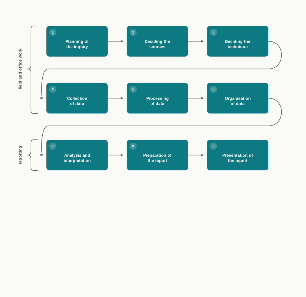
- Planning the inquiry — the objective, scope, population and statistical unit are settled, as explained above.
- Deciding the sources — the investigator settles whether the figures are to be collected first-hand from respondents or taken from records already compiled by some other agency.
- Deciding the technique — the investigator settles whether every unit in the population is to be covered or only a selected part of it.
- Collection of data — the first practical step, in which the plan is executed in the field. Since the data collected are the raw material of every later calculation, they must be accurate, reliable, representative and free from bias.
- Processing of data — the work now shifts from the field to the office, where the entries are checked, edited, coded and transferred to a computer or other record.
- Organisation of data — the processed figures are classified into groups and tabulated so that their significant features stand out.
- Analysis and interpretation — the organised figures are analysed by means of averages, percentages and other statistical measures, and inferences are drawn from them.
- Preparation of the report — the findings, the conclusions drawn and any suggestions arising from them are set down in writing.
- Presentation of the report — the report is placed before those who are to act on it, in a form that is clear, orderly and to the point.
The first three stages are preparation, the next three are the handling of figures, and the last three turn figures into conclusions that somebody can use. Sections 17.2 and 17.3 take up the sources and techniques of collection; the organisation and presentation of data occupy the remainder of the chapter.
17.2 Sources of Data
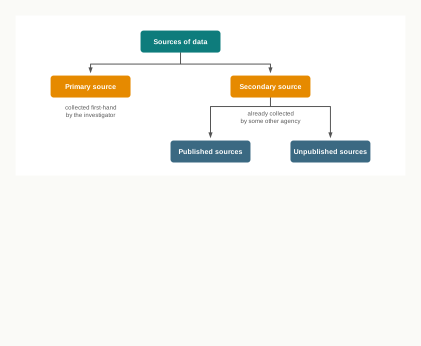
Having settled what it wants to find out, an inquiry must decide where the figures are to come from. There are only two possibilities. Either the investigator goes out and obtains the figures directly from the people or units concerned, or the investigator takes figures that some other agency has already collected and published. The first is the primary source, the second the secondary source.
The choice is a choice between accuracy and cost. Going into the field yields figures shaped exactly to the purpose of the inquiry, but consumes money, time and trained staff. Borrowing figures already compiled costs almost nothing, but they were collected for somebody else’s purpose and may not fit. Fig. 17.2 sets out the two sources and the further division of the secondary source.
17.2.1 Primary Data
Data obtained from the primary source are called primary data. Here the investigator, working through enumerators or field workers, approaches the respondents themselves and records the information at first hand.
Primary Data Primary data are data collected by the investigator himself, directly from the individual respondents, for the purpose of some specific study or inquiry. They are first-hand data, collected from the source of their origin.
Because they are collected for the inquiry in hand, primary data need no adjustment before use: the definitions, the units and the period are all those the investigator chose. They are original in character, and their quality can be checked at every stage. Against this stands their cost, for a field survey needs trained enumerators, transport and time.
Counting Every Person In India In the Census of India, enumerators visit every household in the country and record the age, sex, occupation, education and living conditions of each person. Because the figures are gathered at first hand from the people themselves, they are primary data for the Registrar General’s office that conducts the count. The census of 2011 covered a population of just over 121 crore.
17.2.2 Secondary Data
Data that have already been collected by somebody else, and are used by a later investigator for a purpose of his own, are called secondary data.
Secondary Data Secondary data are data not collected by the investigator himself but obtained from the records and publications of others. They are second-hand data, already collected and processed by some other person or agency.
Secondary data cost little to obtain, since they are simply lifted from reports, journals and official publications, and they may cover a span of years or an area that no single investigator could hope to survey. Their weakness follows from the same fact: they were collected under somebody else’s definitions, for somebody else’s purpose, and often for an earlier period.
Whether a given set of figures is primary or secondary therefore depends not on the figures but on who is using them. Census figures are primary data in the hands of the office that collected them and secondary data in the hands of a student who takes them from the published report.
Never label a set of figures ‘primary’ or ‘secondary’ by itself. The same figures are primary to the agency that collected them and secondary to everyone who uses them afterwards.
17.2.3 Difference between Primary and Secondary Data
The two kinds of data differ in origin, in how far they suit the study in hand, and in what they cost to obtain. The main points of difference are set out below.
Compare Table 17.2 — Primary Data And Secondary Data | Basis | Primary Data | Secondary Data | |—|—|—| | Originality | Original, first-hand data collected from the source of origin | Not original, second-hand data taken from the records of others | | Collecting agency | Collected by the investigator himself through enumerators or field workers | Collected earlier by some other person, agency or department | | Suitability | Collected for a predetermined objective, so they need no adjustment | Collected for another purpose, so they usually need adjustment before use | | Cost of collection | Expensive in money, time and effort | Inexpensive, since they are simply obtained from published reports | | Precautions needed | Care is needed in framing questions and training enumerators | Care is needed in judging the reliability, adequacy and suitability of the figures |
17.2.4 Published Sources of Secondary Data
Most secondary data reach the user in printed or electronic publications. Table 17.2 groups the principal published sources and names an example of each.
Table 17.2 — Published Sources Of Secondary Data | Type of source | Examples | |—|—| | Government publications | Economic Survey, Census of India reports, National Sample Survey reports, Annual Survey of Industries | | Central bank and financial publications | Reserve Bank of India Bulletin, Handbook of Statistics on the Indian Economy | | Semi-government publications | Reports of the Food Corporation of India, birth and death records of municipalities | | Reports of committees and commissions | Reports of the Finance Commission and of Pay Commissions | | International organisations | Human Development Report, World Development Report | | Research institutions and trade bodies | Studies of the National Council of Applied Economic Research and of chambers of commerce | | Journals, newspapers and company reports | Annual reports of joint-stock companies, financial dailies |
These sources differ in coverage and in how often they appear. Some, such as the census, come once in ten years; some, such as the Economic Survey, appear annually; and some, such as the Reserve Bank’s bulletin, appear every month.
17.2.5 Unpublished Sources of Secondary Data
Not all statistical data are published. A great deal exists as internal records kept in the files of government departments and private agencies, and as unpublished material held by research institutions, universities, trade associations, chambers of commerce and individual scholars.
Such records may be used as secondary data with the permission of the organisation concerned. Being unpublished, they have not been through the checking that publication normally involves, so the user must satisfy himself about how they were compiled.
17.2.6 Precautions in the Use of Secondary Data
Secondary data are somebody else’s work, and the user who takes them over takes over their defects as well. Four questions should be settled before they are used.
- Reliability — who collected the figures, by what method, and how competent and impartial was the collecting agency.
- Suitability — whether the definitions, units and period used by the original agency match those of the present inquiry. Figures on ‘income’ are of no use if the original inquiry meant by it something different from what the present one means.
- Adequacy — whether the figures cover the whole area and the whole period the present inquiry deals with, and whether the coverage is wide enough to support the conclusions to be drawn.
- Timeliness — whether the figures are recent enough for the purpose. Old figures may describe conditions that no longer hold.
A question on secondary data usually asks for both the sources and the precautions. Name published and unpublished sources separately, and give the precautions as reliability, suitability, adequacy and timeliness.
Where the answers to these questions are unsatisfactory, and the point at issue is important enough, there is no substitute for collecting the figures afresh. How that is done is the subject of Section 17.3.
17.3 Methods of Collecting Primary Data
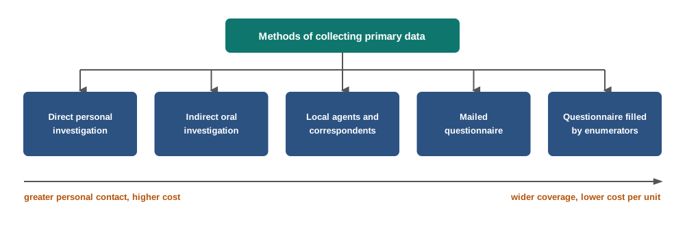
Once an inquiry decides to collect its figures at first hand, it must choose how to approach the respondents. The choice is again governed by the constraint of resources. A method that puts a trained investigator face to face with every respondent gives the most accurate answers and costs the most; a method that mails a form to a wide scattering of people costs least and returns the least dependable answers. Between these lie methods that trade a little accuracy for a large saving in cost and time.
Five methods are in common use, shown in Fig. 17.3.
17.3.1 Direct Personal Investigation
Under direct personal investigation the investigator collects the information personally from the respondents, meeting each one and putting the questions himself. An inquiry into the brands of soap a locality buys would be conducted by calling on the heads of families and asking them directly.
The merits follow from the personal contact. The data are original, collected at their source, and generally accurate, prompt and uniform, since one person asks the questions in one way. Doubts can be cleared on the spot, and the investigator can judge how seriously an answer should be taken.
The limitations follow from the same contact. The method is costly and slow, and becomes impracticable when a large number of persons has to be covered or when they are spread over a wide area. Everything, moreover, rests on the investigator: if he is untrained, or carries a bias or prejudice into the field, the figures will carry it too.
17.3.2 Indirect Oral Investigation
Sometimes the person concerned will not give a truthful answer, or cannot be reached at all. Under indirect oral investigation the information is obtained not from the respondent but from third parties — witnesses — who know enough about the matter to speak of it.
A person who is in debt beyond his means may understate his borrowings; the required information may then be sought from those who know his circumstances. The method is used extensively by committees and commissions appointed by the government, which take evidence from a large number of witnesses and may also seek the opinion of experts.
It is less expensive in money, time and effort than direct investigation and can cover a wide field. Its weakness is that the answers are at one remove from the facts. Witnesses have motives of their own, and their bias passes straight into the data, so the persons examined must be chosen with care.
17.3.4 Mailed Questionnaire
Under this method a questionnaire is sent by post or electronically to the respondents, who are asked to fill it in and return it within a stated time.
Questionnaire A questionnaire is a set of question sheets or forms containing all the questions relating to an inquiry, sent to the respondents so that they may record the required information themselves.
The method is the most economical of all in money, time and effort, and allows a very wide geographical coverage. The information is original, since it comes from the concerned persons themselves.
Its defects are serious. There is no direct contact, so a question misunderstood is a question answered wrongly, and the replies may not be uniform. Many respondents simply do not return the form, and those who do may not be representative of the rest. Above all, the method is useless where the respondents are unable to read and write. It is therefore used mainly by business houses and research organisations dealing with educated and scattered respondents.
17.3.5 Questionnaire Filled by Enumerators
Here a standardised questionnaire is placed in the charge of enumerators, who contact the respondents, put the questions and record the replies in their own handwriting. The form so filled in is called a schedule.
The method has the merits of wide coverage, personal contact with the informants, and a fair degree of uniformity and accuracy, since the enumerators are trained to record answers in one way. It works even where the respondents cannot read or write. It is extensively used for population censuses the world over.
Against this, it is expensive and time-consuming and requires a large body of competent and trained enumerators. For that reason it is generally employed by government institutions and is not suited to private inquiries.
A questionnaire is filled in by the respondent himself. A schedule is the same form filled in by an enumerator on the respondent’s behalf.
The two questionnaire-based methods differ in who does the writing, and everything else follows from that. The main points of difference are set out below.
Compare Table 17.3 — Mailed Questionnaire And Schedule Filled By Enumerators | Basis | Mailed Questionnaire | Schedule Filled by Enumerators | |—|—|—| | Who records the answers | The respondent himself | The enumerator, in his own handwriting | | Contact with the respondent | None; the form travels by post or electronically | Direct personal contact in the field | | Literacy of respondents | Usable only where respondents can read and write | Usable whether or not the respondents are literate | | Cost | Low, since no field staff is needed | High, since a large trained staff is needed | | Accuracy and response | Lower; doubts go uncleared and many forms are never returned | Higher; doubts are cleared on the spot and few units are missed | | Typical users | Business houses and research organisations | Government agencies conducting a census or large survey |
Table 17.3 brings the five methods together for revision.
Table 17.3 — The Five Methods Of Collecting Primary Data Compared | Method | Who supplies the information | Best suited to | Main limitation | |—|—|—|—| | Direct personal investigation | The respondent, in person | Small inquiries over a small area | Costly and slow; open to investigator bias | | Indirect oral investigation | Third parties and witnesses | Inquiries into matters respondents conceal | Answers are second-hand and may be biased | | Local agents and correspondents | Appointed correspondents in each area | Regular information over a wide area | Lack of uniformity; lower accuracy | | Mailed questionnaire | The respondent, in writing | Educated respondents spread widely | Poor response; useless if respondents cannot read | | Questionnaire filled by enumerators | The respondent, recorded by an enumerator | Census and other large official inquiries | Very costly; needs a large trained staff |
17.3.6 Designing a Good Questionnaire
Both the last two methods stand or fall by the quality of the form itself. A badly drafted questionnaire yields answers that no amount of later calculation can repair, so the drafting deserves care.
17.3.6.1 Basic Points in Drafting a Questionnaire
- Covering letter — enclose a letter stating the purpose and usefulness of the inquiry, assuring the respondents that their replies will be kept confidential, and, for a postal inquiry, a self-addressed stamped envelope for the reply.
- Limited number of questions — too few questions yield inadequate information and too many discourage a reply. The number should normally be kept between fifteen and twenty-five.
- Numbering — number the questions, so that both the respondent and the investigator can refer to them without confusion.
- Clarity — keep the questions clear, simple and unambiguous, and avoid technical terms and words carrying more than one meaning.
- Logical arrangement — place the questions in a natural sequence, so that each follows from the last. A question about the number of children should come after, not before, a question about marital status.
- Avoiding certain types of question — leave out questions the respondent will not answer honestly, such as those on the sources of his income, and any that would hurt his social or religious sentiments.
- Objectivity — frame the questions so that the answer is a matter of fact rather than of opinion.
- Definiteness and brevity — frame them so that a definite and short answer is possible.
- Impartiality — avoid controversial questions and any wording that leads the respondent towards a particular answer.
- Avoiding calculation and strain — do not ask questions whose answers require the respondent to calculate, and do not ask him to recall the distant past, since memory is unreliable.
- Cross-checks — build in questions that verify one another, such as asking both the age and the date of birth.
- Clear instructions and attractive layout — state plainly how the form is to be filled in, and leave enough space for the answers.
- Pre-testing — try the draft on a small group of respondents before it is finalised and amend whatever proves difficult to answer. Such a trial is called a pilot survey.
Questions on questionnaire design ask for the essentials, not all of them. Give four or five points with a one-line reason each, and name the pilot survey; a bare list without reasons rarely earns full marks.
17.3.6.2 Types of Questions Used in a Questionnaire
Questions fall into four broad categories, and most questionnaires use a mixture of them.
- Simple alternative questions — the respondent chooses between two answers, such as ‘yes’ and ‘no’ or ‘right’ and ‘wrong’. Example: ‘Does your household own a bicycle? Yes / No’.
- Multiple-choice questions — several alternative answers are printed and the respondent ticks one. Example: ‘Which fuel does your household use most for cooking? (a) firewood (b) kerosene (c) liquefied petroleum gas (d) electricity’.
- Specific information questions — the respondent supplies an exact fact in a word or a figure. Example: ‘How many members are there in your household?’
- Open-ended questions — the respondent gives his views in his own words. Example: ‘What in your view is the chief difficulty in getting farm produce to the market?’
The first three yield answers that can be counted and tabulated at once. Open-ended questions yield richer material but cannot be processed into a frequency table without further classification, so they are used sparingly.
17.4 Census and Sample Methods of Collection
Deciding where the figures will come from settles only half the question. The investigator must also decide how many units to approach. Either every unit belonging to the inquiry is covered, or only a selected part of them is covered and the rest are left out. The first is the census method, the second the sampling method.
This is the sharpest instance of scarcity in the whole business of collecting data. Complete coverage gives figures about which nothing has to be assumed, and costs the most; partial coverage costs a fraction as much and buys that saving with a margin of uncertainty about the units never visited.
17.4.1 Population and the Statistical Unit
Both methods begin from the same starting point — the group the inquiry is about. In statistics this group is called the population or universe.
Population In statistics, the population or universe is the totality of all the persons, objects or items relating to the inquiry under investigation.
The word is used in a special sense here and carries no suggestion of people. If an inquiry concerns the working life of the tube lights in a factory, the population is all the tube lights in that factory. If it concerns the monthly spending of the students of a school on cold drinks, the population is all the students of that school, and each student is the statistical unit.
Population in statistics means every item covered by the inquiry, whether those items are people, firms, fields or machines. It is not the number of inhabitants of a place.
17.4.2 The Census Method
Under the census method every single unit of the population is enumerated. Nothing is left to inference, because nothing is left out.
Census Method The census method is that method in which the required statistical information is collected from each and every unit constituting the population or universe relating to the inquiry.
Suppose the average monthly expenditure of the two thousand students of a school on cold drinks is to be found. Under this method the expenditure of each of the two thousand students is recorded, and the average is worked out from all two thousand figures.
The merits are those of completeness. The information obtained is direct, highly accurate and reliable, and free from the possibility of an unrepresentative selection. Because every unit is covered, the results can be broken down for any subgroup afterwards — by state, by age or by occupation — which is why national counts of population yield exhaustive information on the size, age and sex composition of the people, the occupational structure and the rural-urban distribution.
The demerits are those of scale. The method is very costly and very time-consuming, and it needs a large body of trained and reliable enumerators. It is therefore used only by governments and by a few large institutions, and only where complete coverage is genuinely required.
17.4.3 The Sampling Method
Under the sampling method only a part of the population is studied, and what is found in that part is taken to hold for the whole.
Sample A sample is a selected group of representative units drawn from the population. Under the sampling method, data are collected from this selected number of units and inferences are drawn from them about the entire population.
In the school inquiry, a few students would be selected from each class and their expenditure recorded, and the average so obtained would be taken as an estimate of the average for all two thousand. Fig. 17.4 sets the two methods side by side.
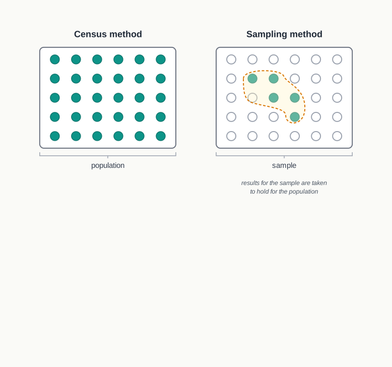
The method is economical, quick and convenient, and for that reason is widely used. It has a further and less obvious merit: because the number of units is small, more care can be taken over each one, so a sample carefully collected may be more accurate in its details than a hurried complete count. It is particularly suitable where the population is very large and its units are broadly similar to one another.
Its demerit is the risk of a biased selection. If the units chosen are not representative of the population, the inference drawn from them will be wrong, and no amount of calculation afterwards will reveal the error. Selecting a sample that genuinely represents the population is the central difficulty of the method.
Estimating A Crop Without Harvesting It State agriculture departments estimate the yield of foodgrain crops through crop-cutting experiments — small plots of fixed size are marked out in selected fields, harvested separately and weighed. No agency could weigh the produce of every field in India, so the yield of the selected plots is used to estimate the yield of the whole crop.
17.4.4 Difference between the Census and Sample Methods
The two methods differ in coverage, and their differences in cost, time and reliability all follow from that one difference. The main points of difference are set out below.
Compare Table 17.4 — The Census Method And The Sampling Method | Basis | Census Method | Sampling Method | |—|—|—| | Coverage | Every unit of the population is enumerated | Only selected representative units are studied | | Cost | Very high, since the whole population is covered | Low, since only a part is covered | | Time | Long | Short | | Staff required | A large body of trained enumerators | A small team | | Nature of the result | An actual figure for the population | An estimate of the population figure, drawn by inference | | Chief risk | Errors of enumeration over so vast an operation | A biased or unrepresentative sample | | Suitability | Where complete coverage is essential and resources permit | Where the population is large and its units broadly similar |
The choice between them is therefore not a matter of one being better than the other. Where the population is small, or where a figure is needed for every subgroup within it, the census method is worth its cost. Where the population is large and reasonably uniform, sampling gives an answer good enough for the purpose at a small fraction of the expense.
Questions on this pair often ask which method suits a stated situation. Decide by the size of the population and by whether every unit must be covered — estimating a country’s population needs a census, estimating the average spending of a school’s students does not.
17.5 Organisation of Data
The field work is now over and the figures are in hand. What the investigator possesses at this point is a mass of raw data — accurate, perhaps, and dearly bought, but shapeless. Before anything can be learnt from it, it has to be put in order.
17.5.1 Why Raw Data Must Be Organised
A small set of figures can be read as it stands. Where the figures run into hundreds or thousands, they are unwieldy, unorganised and haphazard, and no reader can hold them in his mind at once. The eye can take in ten marks; it cannot take in the marks of four hundred candidates written out one after another.
The difficulty is not that the raw data are incomplete. Everything the inquiry found is there. The difficulty is that the information is buried in the bulk: the figures carry facts about the group as a whole — how large the items typically are, how widely they differ, where they cluster — and none of these facts is visible until the figures are condensed.
Organisation is the work of condensing them. It sacrifices detail deliberately, since two hundred separate entries become a table of eight classes and the individual entries disappear, and it buys in exchange a picture of the whole that the entries could never have given.
17.5.2 Meaning of Organisation of Data
Organisation of Data Organisation of data refers to the arrangement of data in a condensed form and their proper and suitable grouping through classification and tabulation.
Two operations are involved, and they are performed in that order. Classification divides the whole body of data into a number of groups or classes, each holding items that share some common characteristic. Tabulation then sets the classified figures out in well-designed and systematic tables.
The two are distinct. Classification is concerned with dividing the data; tabulation is concerned with arranging and presenting what the division has produced. Classification is taken up in Section 17.6 and tabular presentation in Section 17.8.
A Dealer’s Sales Register A wholesale dealer’s register records every sale of the day in the order it happened — a hundred and forty entries by closing time. Read straight through, it shows nothing. Grouped by item and totalled, the same entries show at once which goods are moving, which are idle and where the day’s takings came from.
17.5.3 Variables and Attributes
Data are collected about the characteristics of the units studied, and those characteristics are of two kinds. Some can be measured and stated as a number; others can only be observed as present or absent.
Variable A variable is a characteristic that can be measured and expressed in numerical and quantitative terms, and whose value differs from one item to another.
Height, weight, age, income, price and volume of sales are all variables, because each takes a numerical value that varies from one unit to the next. When a phenomenon assumes different values in this way it is called a variable in statistics, and classification according to it is known as classification by variables.
Attribute An attribute is a qualitative characteristic which cannot be measured numerically, such as sex, nationality, marital status, colour of eyes or literacy. It can only be found to be present or absent in a unit.
Where the characteristic is an attribute, all that can be recorded is which units possess it and which do not. If the attribute under study is literacy, an individual can only be counted as literate or illiterate; there is no numerical value to measure. The units are therefore classified by the presence or absence of the attribute in them.
Compare Table 17.5 — Variable And Attribute | Basis | Variable | Attribute | |—|—|—| | Nature | Quantitative characteristic | Qualitative characteristic | | Measurement | Can be measured and stated as a number | Cannot be measured; only presence or absence can be noted | | Examples | Height, income, marks, price | Sex, literacy, marital status, nationality | | Basis of classification | Units are grouped by the numerical values of the characteristic | Units are grouped by whether they possess the characteristic | | Type of classification | Quantitative classification | Qualitative classification |
A characteristic recorded in numbers is not always a variable. A code number given to each state, or a roll number given to each student, is only a label and measures nothing.
17.5.4 Discrete and Continuous Variables
Variables themselves divide into two kinds according to the values they are capable of taking.
A discrete variable takes only exact or separate values, with gaps between them and nothing in between. The number of children in a family is discrete: a family may have two children or three, but not 2.5. So are the number of workers in a factory and the number of rooms in a house, all of which are counted in whole numbers.
A continuous variable can take any numerical value, whole or fractional, within a certain range. The height of a student may be 160 centimetres, or 160.1, or 160.25, or any value between; height is measured rather than counted, and measurement can always be made finer.
The distinction governs how a variable is later organised into a series, as Section 17.7 will show: a discrete variable is set out against its exact values, a continuous one against classes such as 10–15 or 15–20. Table 17.4 classifies some common characteristics.
Table 17.4 — Characteristics Classified As Attributes, Discrete Variables And Continuous Variables | Characteristic | Attribute or variable | If a variable, discrete or continuous | |—|—|—| | Marital status of a person | Attribute | — | | Number of members in a household | Variable | Discrete | | Monthly income of a household (₹) | Variable | Continuous | | Literacy of a person | Attribute | — | | Number of cars owned by a family | Variable | Discrete | | Daily wage of a worker (₹) | Variable | Continuous | | Weight of a wheat bag (kg) | Variable | Continuous | | Nationality of a person | Attribute | — |
The test for a discrete variable is whether a value between two neighbouring values is possible. If it is, the variable is continuous. Money amounts are treated as continuous even though they stop at the paisa.
17.6 Classification of Data
Organising data begins with classification. Until the items have been sorted into groups, no table can be drawn and no average can be found, because there is nothing to count.
17.6.1 Meaning of Classification
Classification of Data Classification of data is the process of arranging raw data into different groups or classes according to some common characteristic or criterion, so that items alike in that respect are placed together and items unlike are placed apart.
The idea is familiar from ordinary life. Letters at a post office are sorted by the town they are addressed to, and books in a school library are shelved by the subject they deal with. In each case a single characteristic is chosen and everything is arranged by it, so that any item can be found and any group can be counted.
Statistical classification works the same way. Students may be grouped by the marks they obtained, or people by their age or their monthly income. What decides the grouping is the purpose of the inquiry, since the characteristic chosen is the one whose effect the inquiry wishes to see.
Classification and tabulation are two steps, not one. Classification divides the data into groups; tabulation then arranges those groups in rows and columns.
17.6.2 Objectives of Classification
- Simplification — it presents a mass of complex data in a simple, condensed and logical form, so that the whole body can be taken in at once.
- Scientific arrangement — it arranges the data in an orderly manner, which is the necessary preparation for every later statistical operation.
- Utility — it brings out the points of similarity and dissimilarity among the items and so raises the usefulness of the data.
- Distinctive features — it makes the significant features of the data stand out, which the raw figures conceal.
- Comparability — it makes comparison possible, between one group and another or between one period and another, and so allows inferences to be drawn.
- Relationship — it helps in finding out the relationship among the various characteristics of the data, such as that between literacy and income.
17.6.3 Types of Classification
Data can be classified on four bases — place, time, quality and quantity — and these give the four types shown in Fig. 17.5.
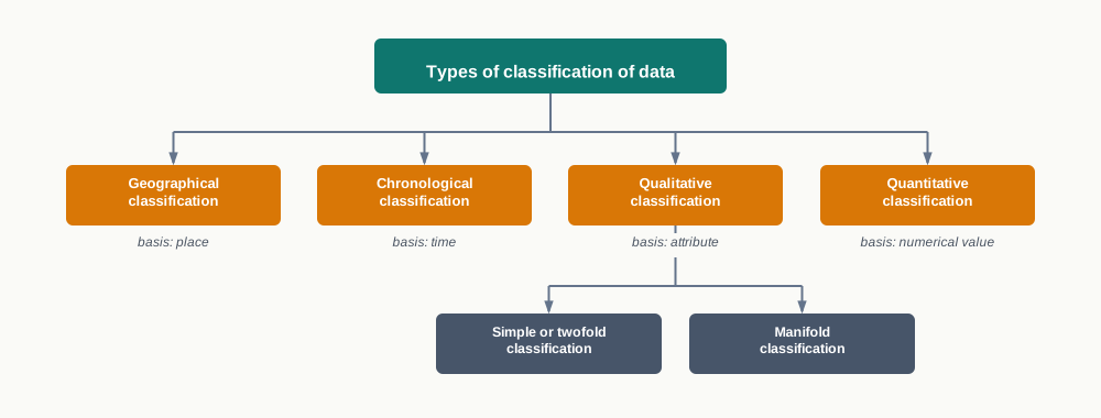
Each is taken up in turn below.
17.6.4 Geographical Classification
In geographical classification the data are classified on the basis of place — by village, district, state or country. It is also called spatial classification. The output of wheat in India, for instance, may be set out state by state, or the population of the country may be shown for each state separately.
The arrangement within such a classification is usually alphabetical, or by the size of the figure, so that the largest and smallest areas can be seen at a glance.
17.6.5 Chronological Classification
In chronological classification the data are classified on the basis of time — by week, month, quarter, year or decade. Data so arranged are also called time series data.
The population of India shown for each census year in turn, or the annual output of foodgrains shown year by year, is a chronological classification. Its value lies in showing movement: only when the same figure is set down for successive periods can a rise, a fall or a turning point be seen.
17.6.6 Qualitative Classification
In qualitative classification the data are classified on the basis of some attribute, that is, some characteristic that cannot be measured. Since an attribute can only be present or absent, the units are grouped by whether they possess it. Qualitative classification is of two kinds.
17.6.6.1 Simple or Twofold Classification
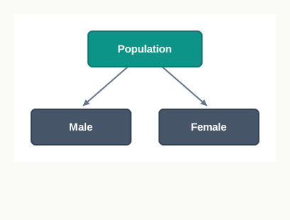
Where the data are classified by the presence or absence of a single attribute, the classification is simple or twofold. There are then exactly two classes: those possessing the attribute and those not possessing it. Classifying a population by sex, into males and females, is a simple classification, as Fig. 17.6 shows.
17.6.6.2 Manifold Classification
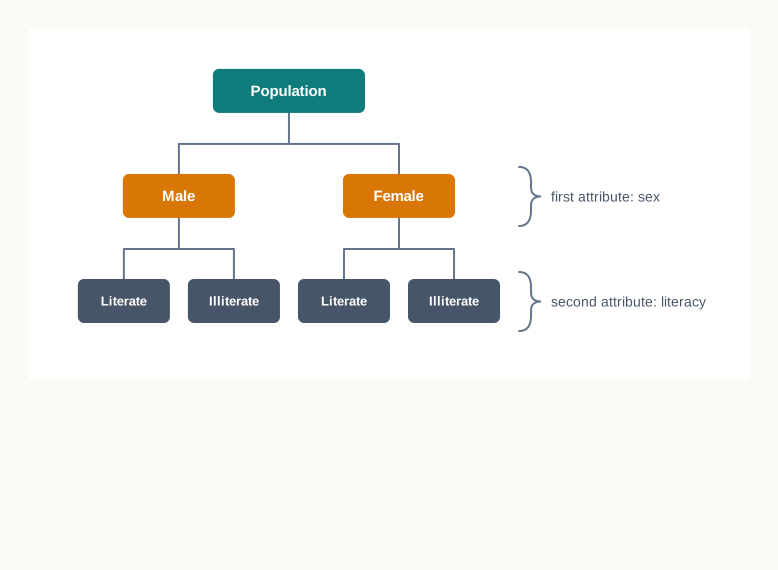
Where the data are classified by more than one attribute, one after another, the classification is manifold or multiple. The population may first be divided by sex into males and females, and each of those two classes then divided by literacy into literate and illiterate, giving four classes in all. Fig. 17.7 shows the arrangement.
17.6.7 Quantitative Classification
In quantitative classification the data are classified according to a characteristic that can be measured — height, weight, income, birth rate or marks obtained. Here the units are grouped by their numerical values, so that students may be arranged by the marks they scored or workers by their daily wages.
Since a measurable characteristic that takes different values is a variable, quantitative classification is also known as classification by variables. It is the type that leads directly to the frequency distributions of Section 17.7, and it is the type on which almost all later statistical work is done.
Table 17.5 — The Four Types Of Classification Illustrated | Type | Basis of classification | Illustration | |—|—|—| | Geographical | Place | Foodgrain output shown separately for each state | | Chronological | Time | Population of India shown for each census year | | Qualitative | Attribute | Workers classified as literate and illiterate | | Quantitative | Numerical value of a variable | Workers classified by daily wage into ₹300–400, ₹400–500 and so on |
The last two types are the ones commonly confused, and the difference between them is worth fixing.
Compare Table 17.6 — Qualitative And Quantitative Classification | Basis | Qualitative Classification | Quantitative Classification | |—|—|—| | Characteristic used | An attribute, which cannot be measured | A variable, which can be measured | | How classes are formed | By the presence or absence of the attribute | By the numerical values or class intervals of the variable | | Examples | Sex, literacy, marital status, nationality | Height, income, marks, daily wage | | Number of classes | Two under simple classification, more under manifold | As many as the chosen class intervals give | | Also known as | Classification according to attributes | Classification by variables |
Four Ways Of Looking At India’s Workers One body of survey data on workers can be classified four ways over. By place, workers divide into rural and urban; by time, the same figure is set down for successive survey rounds; by attribute, workers are grouped as male and female; and by variable, as earning under ₹10,000 a month, ₹10,000 to ₹20,000, and so on. The data never change — only the question being asked of them.
Name the basis, not just the type. A one-mark answer that says ‘geographical classification’ earns little; ‘classification on the basis of place, such as state-wise output’ earns the mark in full.
17.7 Statistical Series
Classification tells us on what basis the items are to be grouped. A statistical series is what the grouping actually produces — the data set out in a logical order, ready to be tabulated, averaged and compared.
Statistical Series A statistical series is a set of data arranged in some logical order, so that the items can be read against the values of the characteristic being studied.
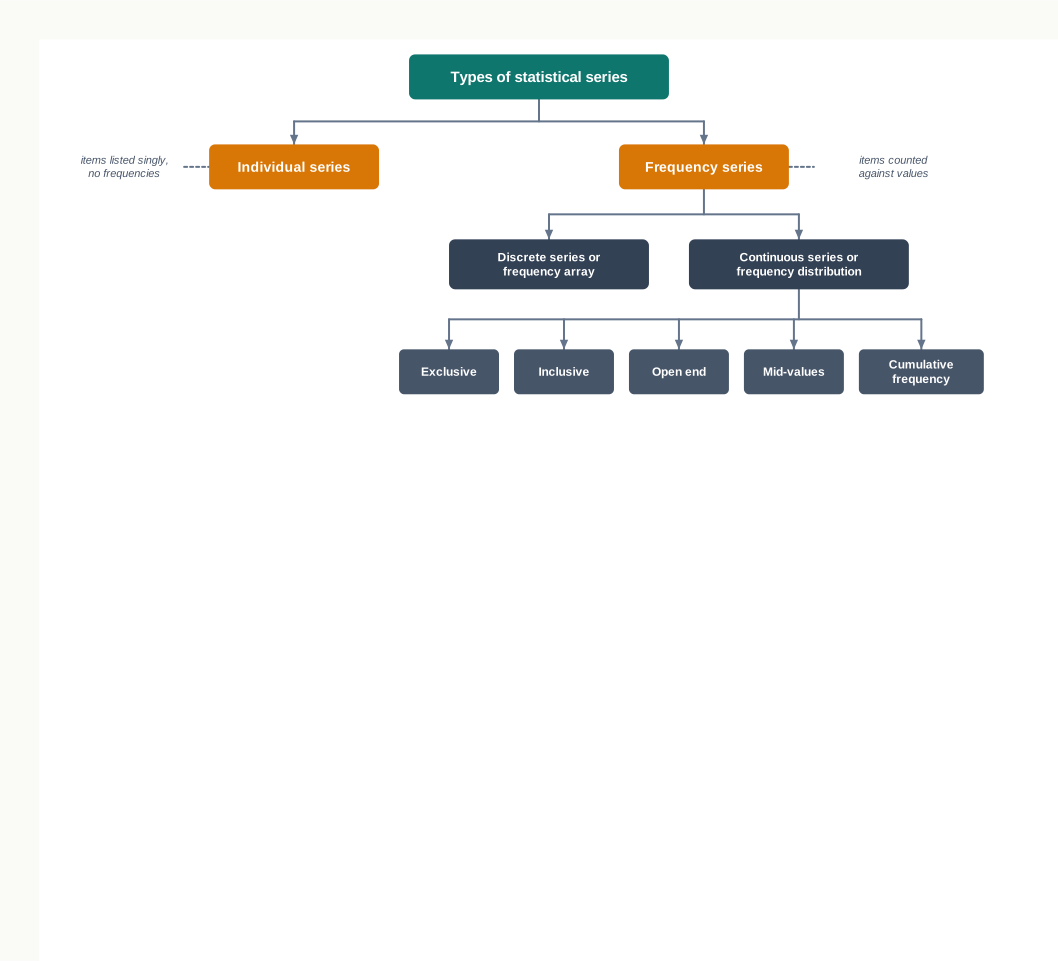
Series differ according to the nature of the variable. Where every item is listed separately the series is individual; where items are counted against the values they take, the series carries frequencies. Fig. 17.8 sets out the whole family.
17.7.1 Individual Series
In an individual series each item is listed singly and has its own value. Nothing is grouped and no frequencies appear. The daily wages earned by each worker in a small workshop, or the marks obtained by each student in a class, can be listed in this way.
Such a series can be arranged in two ways. Under serial order the items are listed in the order in which they were recorded — by roll number, by token number, by date. Under a simple array they are arranged by magnitude, either ascending, with the smallest first, or descending, with the largest first.
SE 17.1 — Arranging An Individual Series
The daily wages, in rupees, paid to ten workers of a workshop on a particular day were recorded token number by token number as: 420, 385, 500, 360, 445, 500, 390, 415, 470, 430. Present these data as an individual series in serial order and as an ascending array, and state the range.
In serial order, by token number 420, 385, 500, 360, 445, 500, 390, 415, 470, 430
As an ascending array 360, 385, 390, 415, 420, 430, 445, 470, 500, 500
Lowest wage ₹360
Highest wage ₹500
Range = highest − lowest ₹500 − ₹360 = ₹140
The array shows that the ten wages lie within a band of ₹140, which the serial order does not reveal.
An individual series is simple to prepare and keeps every figure intact. That is also its limitation: where the number of items is large, listing them singly leaves the data as unwieldy as before.
17.7.2 Frequency and Frequency Distribution
The way out is to stop listing items and start counting them. The number of times a particular value occurs in the data is called its frequency.
Frequency The frequency of a value is the number of times that value occurs in the given data. A table showing the values of a variable together with their corresponding frequencies is called a frequency distribution.
Counting is done with the help of tally bars. As the investigator goes through the raw data item by item, a vertical stroke is entered against the value that item takes. Every fifth stroke is drawn across the preceding four, so that the marks fall into blocks of five and can be totalled quickly at the end. The total of the strokes against a value is its frequency, and the sum of all the frequencies, written \(\sum f\), equals the number of items in the data. In the tally columns of this chapter a completed block of five is printed as four upright strokes crossed by a fifth.
17.7.3 Discrete Series or Frequency Array
Where the variable is discrete, each of its exact values can be shown separately with the number of items taking that value. Such a series is a discrete series or frequency array.
Three columns are needed: the values of the variable in the first, arranged in ascending or descending order; the tally bars in the second; and the total frequency in the third. The tally column is working, and is dropped when the finished series is presented.
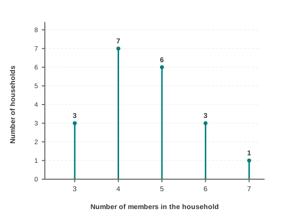
Table 17.6 — Working For The Frequency Array Of Household Size | Number of members (1) | Tally bars (2) | Frequency, f (3) | |—|—|—| | 3 | III | 3 | | 4 | IIII II | 7 | | 5 | IIII I | 6 | | 6 | III | 3 | | 7 | I | 1 | | Total | — | 20 |
SE 17.2 — Preparing A Frequency Array
Twenty households in a locality were surveyed to find how many members each had. The replies were: 4, 5, 3, 6, 4, 4, 5, 3, 7, 4, 5, 6, 4, 3, 5, 4, 6, 5, 4, 5. Prepare a frequency array of the number of members; the tally work is set out in Table 17.6.
From Table 17.6, the values taken by the variable 3, 4, 5, 6 and 7 members
Frequency of 3 members 3 households
Frequency of 4 members 7 households
Frequency of 5 members 6 households
Frequency of 6 members 3 households
Frequency of 7 members 1 household
\(\sum f\) 20 households
The twenty separate replies have become a series of five values, and it is now visible at once that households of four members are the commonest.
A frequency array works only while the variable takes a few exact values. Where the values run into scores or hundreds, a separate line for each is no improvement on the raw data at all.
17.7.4 Continuous Series or Frequency Distribution
Where the variable is continuous, or where a discrete variable takes too many values to list, the items are grouped into ranges. Such a series is a continuous series or frequency distribution, and is also called a series of grouped data.
A range of values within which a set of items falls is a class, such as 20–30 or 30–40. The lowest and highest values of a class are its class limits: the lower limit and the upper limit. The difference between them is the class interval or class size.
Class Interval The class interval, or class size, is the span or width of a class, obtained as the difference between its upper limit and its lower limit. For the class 20–30, the class interval is \(30 - 20 = 10\).
The value lying exactly half-way between the two limits is the mid-value or class-mark, obtained by adding the two limits and dividing by two.
\[m = \dfrac{l_1 + l_2}{2}\]
Here \(m\) is the mid-value of the class, \(l_1\) its lower limit and \(l_2\) its upper limit, all in the units of the variable. The mid-value of the class 20–30 is \(\dfrac{20 + 30}{2} = 25\). It represents the whole class in every later calculation, on the assumption that the items in a class are spread evenly across it.
Income Tax Slabs Are Class Intervals Personal income tax is charged not on each income separately but on slabs — bands of income, each with a lower and an upper limit, with one rate applied to all income falling inside a band. A schedule that treated every income figure separately would be unusable. Grouping into classes is what makes the tax schedule short enough to print and simple enough to apply.
17.7.5 Construction of a Frequency Distribution
Four steps turn raw data into a frequency distribution.
- Arrange the raw data as an array, so that the lowest and highest values can be seen and the range found.
- Decide the number of classes and the class size. The number of classes should generally lie between six and fifteen, and the class size should be uniform and, as far as possible, 5 or a multiple of 5.
- Write out the classes in a three-column table, with the classes in the first column, tally bars in the second and frequencies in the third.
- Go through the data item by item, entering a tally against the class each item falls in, and total the tallies to obtain the class frequencies.
Too few classes hide the pattern by lumping unlike items together; too many scatter the items so thinly that each class holds almost nothing. The choice of class size is a judgement between these two losses.
Table 17.7 — Working For The Frequency Distribution Of Marks Of Forty Students | Marks (1) | Tally bars (2) | Frequency, f (3) | |—|—|—| | 20–30 | IIII | 4 | | 30–40 | IIII II | 7 | | 40–50 | IIII IIII | 10 | | 50–60 | IIII IIII | 9 | | 60–70 | IIII I | 6 | | 70–80 | IIII | 4 | | Total | — | 40 |
SE 17.3 — Constructing A Frequency Distribution
The marks obtained out of 100 by forty students of a class were: 45, 33, 24, 55, 63, 41, 72, 36, 52, 27, 48, 58, 66, 31, 43, 75, 21, 38, 51, 47, 61, 34, 56, 29, 44, 68, 53, 39, 40, 57, 71, 49, 64, 32, 42, 59, 78, 46, 54, 69. Prepare a frequency distribution taking a class interval of 10; the tally work is set out in Table 17.7.
Highest value 78 marks
Lowest value 21 marks
Range = highest − lowest 78 − 21 = 57 marks
Class interval taken 10 marks
Number of classes needed 6, running from 20–30 to 70–80
From Table 17.7, \(\sum f\) 40 students
The forty separate marks are now a distribution of six classes, and the class 40–50, holding 10 students, is the one in which marks are thickest.
17.7.6 Types of Frequency Distribution Series
Frequency distributions are of five types, according to how the classes are written.
17.7.6.1 Exclusive and Inclusive Series
In an exclusive series the items corresponding to the upper limit of a class are excluded from that class and counted in the next. The upper limit of one class is therefore the lower limit of the next, as in 10–20, 20–30, 30–40. A student scoring 20 marks goes into the class 20–30, not into 10–20, so the class 10–20 in fact holds values from 10 up to 19 and their fractions.
In an inclusive series all items up to and including the upper limit are counted in that class. The classes therefore do not repeat a limit, and are written 10–19, 20–29, 30–39, with a gap between the upper limit of one class and the lower limit of the next. A student scoring 19 marks and one scoring 10 marks both fall in the class 10–19.
In an exclusive series the upper limit belongs to the next class, not to its own. An item of value 30 in the classes 20–30 and 30–40 is counted in 30–40.
Compare Table 17.7 — Exclusive Series And Inclusive Series | Basis | Exclusive Series | Inclusive Series | |—|—|—| | Treatment of the upper limit | Excluded from the class and counted in the next | Included in the class itself | | Form of the classes | The upper limit repeats as the next lower limit, as in 10–20, 20–30 | Limits do not repeat, as in 10–19, 20–29 | | Gap between classes | No gap; the classes are continuous | A gap of 0.1 to 1.0 between one class and the next | | Suitability | Suited to a continuous variable | Suited to a discrete variable | | Use in calculation | Ready for use as it stands | Must be converted to the exclusive form before most calculations |
17.7.6.2 Open End and Mid-Values Series
An open end series is one in which the lower limit of the first class, or the upper limit of the last class, or both, are missing. In their place stand ‘less than’ or ‘below’ at the bottom and ‘more than’ or ‘above’ at the top, as in Table 17.8.
Table 17.8 — An Open End Series Of Ages | Age in years | Number of persons | |—|—| | Below 10 | 7 | | 10–20 | 8 | | 20–30 | 12 | | 30–40 | 6 | | Above 40 | 4 |
Open classes are used where a few items lie far from the rest, and where fixing a limit for them would create a long stretch of empty classes. Where the class interval is uniform through the rest of the series, the open classes may be closed by giving them the same interval — here the first class becomes 0–10 and the last 40–50.
A mid-values series gives only the mid-value of each class and its frequency, leaving the limits unstated, as in Table 17.9.
Table 17.9 — A Mid-Values Series | Mid-value | 5 | 15 | 25 | 35 | 45 | |—|—|—|—|—|—| | Frequency | 7 | 8 | 12 | 6 | 4 |
The limits can be recovered in three steps. Take the difference between two consecutive mid-values, here \(15 - 5 = 10\); halve it, giving \(\dfrac{10}{2} = 5\); then subtract that half from each mid-value for the lower limit and add it for the upper. The first class is therefore \(5 - 5 = 0\) to \(5 + 5 = 10\), and the remaining classes are 10–20, 20–30, 30–40 and 40–50.
17.7.6.3 Cumulative Frequency Series
In a cumulative frequency series the frequencies are added up progressively, class by class, so that each entry shows how many items lie below or above a stated value.
Cumulative Frequency The cumulative frequency of a class is the total of its own frequency and the frequencies of all the classes preceding it, under the ‘less than’ method, or of all the classes following it, under the ‘more than’ method.
A less than series is built by starting from the first class and adding downwards, and it shows how many items fall below each upper limit. A more than series is built by starting from the last class and adding upwards, and it shows how many items lie above each lower limit. Table 17.10 sets out both for the distribution of marks found in SE 17.3.
Table 17.10 — Less Than And More Than Cumulative Frequency Distributions Of Marks | Marks | Frequency, f | Less than (upper limit) | Cumulative frequency (less than) | More than (lower limit) | Cumulative frequency (more than) | |—|—|—|—|—|—| | 20–30 | 4 | Less than 30 | 4 | More than 20 | 40 | | 30–40 | 7 | Less than 40 | 11 | More than 30 | 36 | | 40–50 | 10 | Less than 50 | 21 | More than 40 | 29 | | 50–60 | 9 | Less than 60 | 30 | More than 50 | 19 | | 60–70 | 6 | Less than 70 | 36 | More than 60 | 10 | | 70–80 | 4 | Less than 80 | 40 | More than 70 | 4 |
Each series can be turned back into the simple frequencies it came from. Under the ‘less than’ form, the frequency of a class is found by deducting from its cumulative frequency the cumulative frequency of the class before it: the frequency of 40–50 is \(21 - 11 = 10\). Under the ‘more than’ form, the frequency of a class is found by deducting from its cumulative frequency that of the class after it: \(29 - 19 = 10\) again.
Cumulative frequencies are the basis of the median, the quartiles and the ogive. Always check that the last entry of a ‘less than’ series and the first entry of a ‘more than’ series both equal \(\sum f\); if they do not, the addition has gone wrong.
17.8 Tabular Presentation of Data
The data have been collected, classified and formed into a series. What remains is to place them before a reader in a form he can take in — and a reader who cannot take them in gains nothing from all the work that went before.
17.8.1 Meaning and Purpose of Presentation of Data
Presentation of Data Presentation of data refers to the various ways in which data are set out so that they may be easily and clearly understood and analysed.
Presentation is not decoration. Classified data are still rows of figures, and the pattern in them becomes visible only when they are laid out in a form the eye can follow. A well-presented table or diagram makes the comparison the inquiry was undertaken to make, and does it at a glance.
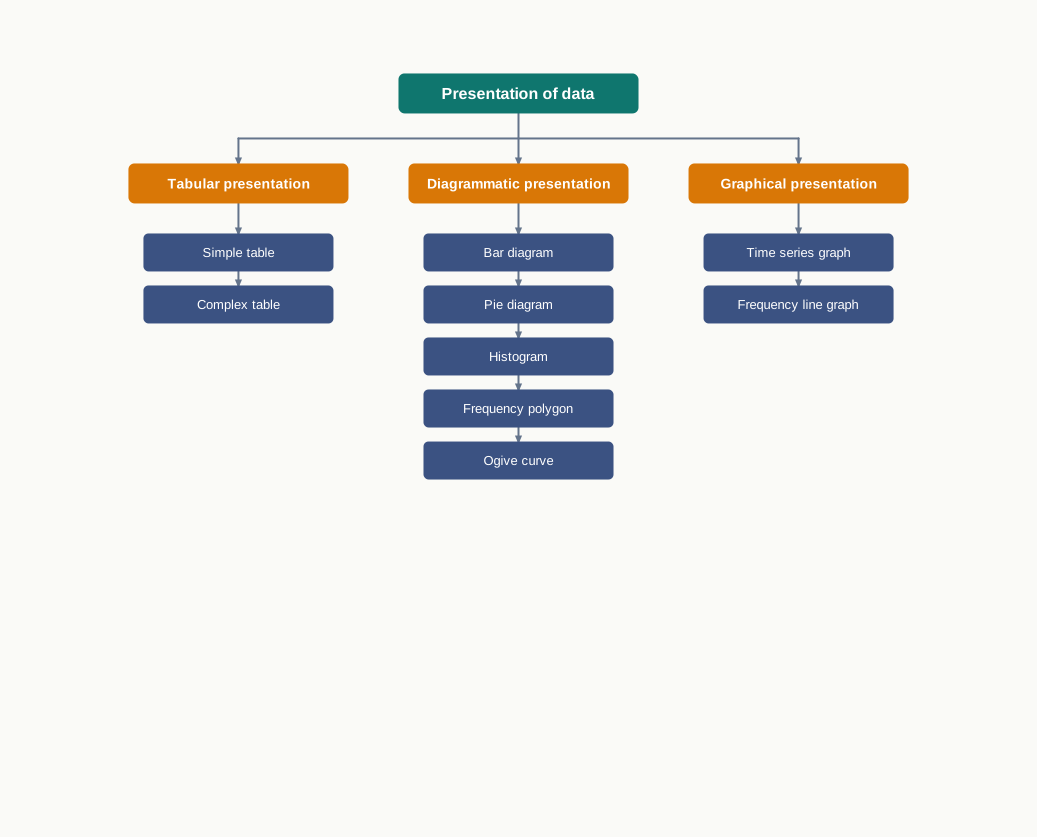
Data may be presented in three forms, shown in Fig. 17.9: in tables, in diagrams and in graphs. Tabular presentation is taken up in this section, diagrammatic presentation in Section 17.9 and graphical presentation in Section 17.10.
17.8.2 Meaning of a Statistical Table
Statistical Table A statistical table is a systematic organisation of data in columns and rows, so that each figure can be read against the two characteristics that locate it.
The strength of a table is that it fixes every figure by position. A reader finds the row he wants and the column he wants, and the figure standing where they cross is the one he is after. That is why tabulation is the simplest, most economical and most widely used form of presentation, and why almost every diagram and graph in this chapter is drawn from a table first.
17.8.3 Parts of a Statistical Table
A table has nine parts, and each has a settled place, shown in Fig. 17.10.
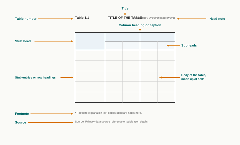
- Table number — every table is numbered so that it can be referred to. In this book the number carries the chapter first, so that Table 17.6 is the sixth table of Chapter 17.
- Title — a short, clear statement, printed above the table, of exactly what the table shows. It should name the characteristic, the place and the period.
- Head note — a brief note in brackets, placed at the top right, giving the units in which the figures are stated or the period they cover, such as ‘in ₹ crore’ or ‘in tonnes’.
- Stub head — the heading of the first column, describing what the rows stand for.
- Stub entries — the row headings themselves, which identify the information contained in each row, such as the different years.
- Caption or column heading — the heading given to each column, describing what the figures in it stand for.
- Subheads — where a column heading divides into parts, as when a column for students divides into boys and girls, the parts are given subheads beneath the main caption.
- Body of the table — the figures themselves. Each individual figure is called a cell, and is fixed by the row and column it stands in.
- Footnote and source — the footnote explains anything in the table that needs qualifying, and the source names the publication the figures were taken from, with its year. A source line is required whenever the data are secondary.
The caption heads the columns and the stub heads the rows. A table read with the two interchanged gives figures that look plausible and mean nothing.
Why Official Tables Carry A Source Line Statistical tables in government publications such as the Economic Survey almost always carry a head note stating the unit and a source line naming the ministry or agency that supplied the figures. This lets a reader check the original, see how the figures were defined, and know which year’s estimate he is looking at — the same precautions Section 17.2.6 requires of anyone using secondary data.
17.8.4 Simple and Complex Tables
A simple table, also called a one-way table, presents data relating to only one characteristic. Table 17.11 shows the enrolment of a school over five years, and enrolment is the only characteristic recorded.
Table 17.11 — Enrolment In A Secondary School, 2018 To 2022 | Year | Number of students enrolled | |—|—| | 2018 | 620 | | 2019 | 655 | | 2020 | 690 | | 2021 | 712 | | 2022 | 745 |
A complex table presents data relating to two or more characteristics at the same time. If the same enrolment figures are also divided by sex, the table becomes complex, as in Table 17.12, where the caption divides into two subheads.
Table 17.12 — Enrolment In A Secondary School By Sex, 2018 To 2022 | Year | Boys | Girls | Total | |—|—|—|—| | 2018 | 330 | 290 | 620 | | 2019 | 345 | 310 | 655 | | 2020 | 360 | 330 | 690 | | 2021 | 368 | 344 | 712 | | 2022 | 380 | 365 | 745 |
The totals in Table 17.12 are exactly the figures of Table 17.11. Nothing has been added to the data; a second characteristic has simply been brought in, and with it the fact that enrolment of girls rose faster over the five years than that of boys.
The main points of difference are set out below.
Compare Table 17.8 — Simple Table And Complex Table | Basis | Simple Table | Complex Table | |—|—|—| | Characteristics shown | One only | Two or more at the same time | | Also called | One-way table | Two-way or manifold table | | Subheads | Not needed | The caption divides into subheads | | Information yielded | The behaviour of a single characteristic | The behaviour of one characteristic across the classes of another | | Ease of reading | Read at a glance | Needs more care, since each cell is fixed by several headings |
A question asking you to draw a table and explain its parts wants the skeleton labelled, not a table of figures. Show the table number, title, head note, stub, caption, body, footnote and source, and name each part.
17.9 Diagrammatic Presentation of Data
A table fixes every figure exactly, but it still has to be read figure by figure. Where the point to be made is a comparison — this year against last, this item against that — a diagram makes it in one look.
17.9.1 Meaning and Usefulness of Diagrammatic Presentation
Diagrammatic Presentation Diagrammatic presentation is the presentation of data in the form of geometric figures, pictures, maps or curves, so that the main features of the data can be grasped at a glance.
The gain is speed of comprehension, and it is bought at a price. A diagram shows relative size, not exact size: a reader can see that one bar is about twice another, but he cannot read either off to the last unit. A diagram is therefore an aid to a table, never a substitute for one, and the figures should always be available behind it.
Diagrams are of most use where a time series is being shown, or where several groups are being compared. They are of least use where the data are numerous or the variables many, since a crowded diagram conveys less than the plain table it replaced.
17.9.2 Bar Diagrams
A bar diagram presents data as a set of bars or rectangles whose lengths are proportional to the values they stand for. All the bars are of equal width and stand on a common base line at equal distances from one another, so that only their height varies and height alone carries the comparison.
17.9.2.1 Simple Bar Diagram
A simple bar diagram represents a single set of figures, one bar to each item or period. Table 17.13 gives the annual output of a cement factory over five years, and Fig. 17.11 presents it as a simple bar diagram in panel (a).
Table 17.13 — Annual Output Of A Cement Factory, 2018 To 2022 | Year | Output (thousand tonnes) | |—|—| | 2018 | 240 | | 2019 | 265 | | 2020 | 210 | | 2021 | 285 | | 2022 | 310 |
17.9.2.2 Multiple Bar Diagram
A multiple bar diagram represents two or more related sets of figures at the same time. For each period a group of bars is drawn, one bar to each set, and the bars within a group touch one another while the groups stand apart. The bars of a set are shaded alike throughout and identified by a key. Panel (b) of Fig. 17.11 presents the enrolment figures of Table 17.12 in this form.
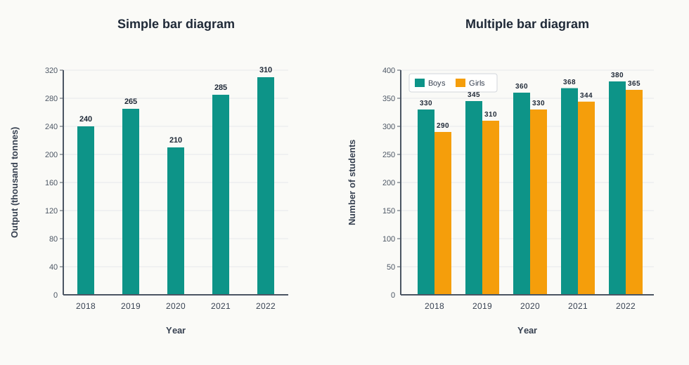
Read together, the two panels show what each form is for. The simple diagram shows how one quantity moved; the multiple diagram shows how two quantities moved in relation to each other.
Bars must be of equal width and equally spaced. Varying the width makes the eye compare areas instead of heights, and the diagram then misstates the data.
17.9.3 Pie Diagram
A pie diagram shows how a total is divided among its components. The whole is drawn as a circle, and the circle is cut into sectors, one to each component, the angle of a sector being proportional to the share of the component in the total.
The angle at the centre of a circle is 360°, and that angle stands for the whole of the quantity being divided. The share of any component is therefore converted into degrees before the sector can be drawn.
\[\text{Angle of a component} = \dfrac{\text{Value of the component}}{\text{Total value}} \times 360°\]
Here the value of the component and the total value are in the same units, and the result is in degrees. Where the components are already expressed as percentages, the same rule reduces to multiplying each percentage by 3.6.
Four steps construct the diagram.
- Express each component as a share of the total, in value or in per cent.
- Convert each share into degrees by the rule above, and check that the degrees add up to 360°.
- Draw a circle and mark a radius, usually vertical, as the starting line.
- Measure off each sector in turn from that line with a protractor, taking the components in order of size, and shade and label each sector.
Table 17.14 sets out the monthly expenditure of a family and its conversion into degrees, and Fig. 17.12 presents it as a pie diagram.
Table 17.14 — Monthly Expenditure Of A Family And Its Conversion Into Degrees | Item | Share of expenditure (per cent) | Angle of the sector (per cent × 3.6) | |—|—|—| | Food | 40 | 144° | | Housing | 20 | 72° | | Education | 15 | 54° | | Transport | 10 | 36° | | Other items | 10 | 36° | | Health | 5 | 18° | | Total | 100 | 360° |
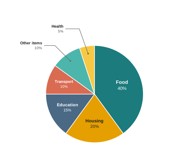
The Rupee Comes And Goes Every Union Budget is accompanied by two pie diagrams, one showing where each rupee of government receipts comes from and the other where each rupee of expenditure goes. Neither adds a single figure to the Budget documents. They exist because a reader can see the size of a sector at once, where he would have to work through pages of tables to reach the same impression.
17.9.4 Histogram
A histogram presents a grouped frequency distribution as a set of adjoining rectangles. Each class is marked off on the X-axis with a width equal to its class interval, and a rectangle is raised on it with a height proportional to the frequency of that class. Since the classes are continuous, the rectangles touch one another.
A histogram is therefore drawn only from grouped data, and only where the series is in the exclusive form. An inclusive series must be converted before the histogram can be drawn, or gaps will appear where none exist in the data.
The rectangles are two-dimensional, and it is the area of each that represents its frequency. Where all the classes are of the same size, height alone shows the frequency, and the histogram can be read like a set of bars — but the two are not the same diagram.
Compare Table 17.9 — Bar Diagram And Histogram | Basis | Bar Diagram | Histogram | |—|—|—| | Data used | Any set of figures, whether classified by attribute, place or time | Grouped frequency distributions only | | Dimension | One-dimensional; only the height of the bar counts | Two-dimensional; the area of the rectangle counts | | Width of the bars | Uniform and arbitrary, chosen for appearance | Fixed by the class interval, and unequal where the classes are unequal | | Spacing | Bars stand apart at equal distances | Rectangles adjoin, since the classes are continuous | | X-axis | Carries items, groups or periods | Carries the values of a continuous variable |
17.9.5 Frequency Polygon
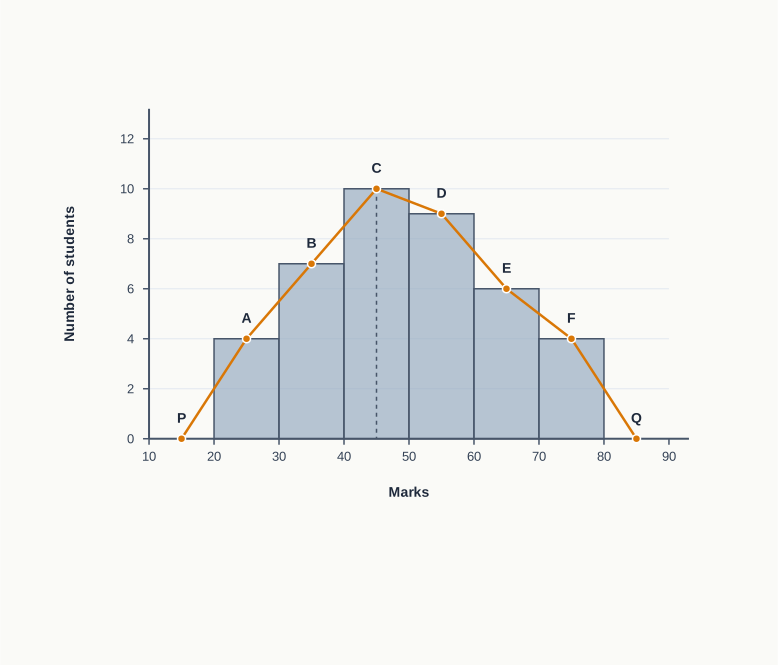
A frequency polygon is obtained by joining the mid-points of the tops of the rectangles of a histogram by straight lines. The curve so drawn has as many sides as there are classes, which is what gives it the name.
The two ends are carried down to the X-axis at the mid-points of the classes immediately below the first and immediately above the last, both of which are taken to have zero frequency. This closes the figure, and it is done so that the area enclosed by the polygon equals the area of the histogram it came from — the polygon cuts off a corner of each rectangle and adds an equal corner outside it.
Fig. 17.13 draws the histogram and the frequency polygon together for the distribution of marks obtained in SE 17.3.
17.9.6 Ogive Curve
An ogive is the curve obtained by plotting a cumulative frequency distribution and joining the plotted points by a smooth curve.
A less than ogive is drawn by plotting each ‘less than’ cumulative frequency against the upper limit of its class. Since the cumulative total can only grow as the upper limits rise, the curve slopes upward from left to right. A more than ogive is drawn by plotting each ‘more than’ cumulative frequency against the lower limit of its class, and slopes downward from left to right for the same reason in reverse.
Fig. 17.14 draws both from the cumulative distributions of Table 17.10.
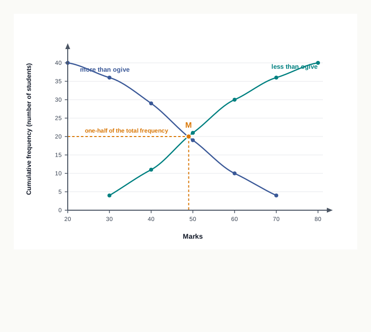
Where the two curves cross, the number of items below that value equals the number above it. The value read off the X-axis at that point is the median of the distribution, a measure taken up in the chapter on measures of central value.
Plot a less than ogive against upper limits and a more than ogive against lower limits. Plotting either against the mid-values is the commonest error, and it displaces the median read off the diagram.
17.10 Graphical Presentation of Data
A diagram compares quantities that stand side by side. A graph does something different: it plots the values of two variables against each other on a pair of axes, so that the relation between them appears as a line.
17.10.1 Meaning of Graphical Presentation
Graphical Presentation Graphical presentation is the presentation of data on a graph, by plotting the values of two variables along the X-axis and the Y-axis and joining the plotted points to obtain a line or curve.
The convention is the usual one. The independent variable — most often time — is measured along the X-axis, and the dependent variable along the Y-axis. Each plotted point fixes one pair of values, and joining the points shows how the second variable moved as the first changed.
What a graph shows that a table cannot is direction and rate of change. A rising line, a flattening line and a line that turns downward each tell the reader something about the movement of the series which no column of figures announces by itself.
17.10.2 Time Series Graphs
A time series graph presents data expressed over successive periods — weeks, months, years or decades. Time is measured along the X-axis and the variable along the Y-axis. Such graphs are of two kinds, according to how many variables are shown.
17.10.2.1 One Variable Graphs
A one variable graph shows the values of a single variable over successive periods. Table 17.15 gives the quantity of milk procured daily by a dairy cooperative over five years, and Fig. 17.15 plots it.
Table 17.15 — Daily Milk Procurement Of A Dairy Cooperative, 2018 To 2022 | Year | Milk procured (thousand litres a day) | |—|—| | 2018 | 42 | | 2019 | 48 | | 2020 | 51 | | 2021 | 57 | | 2022 | 64 |
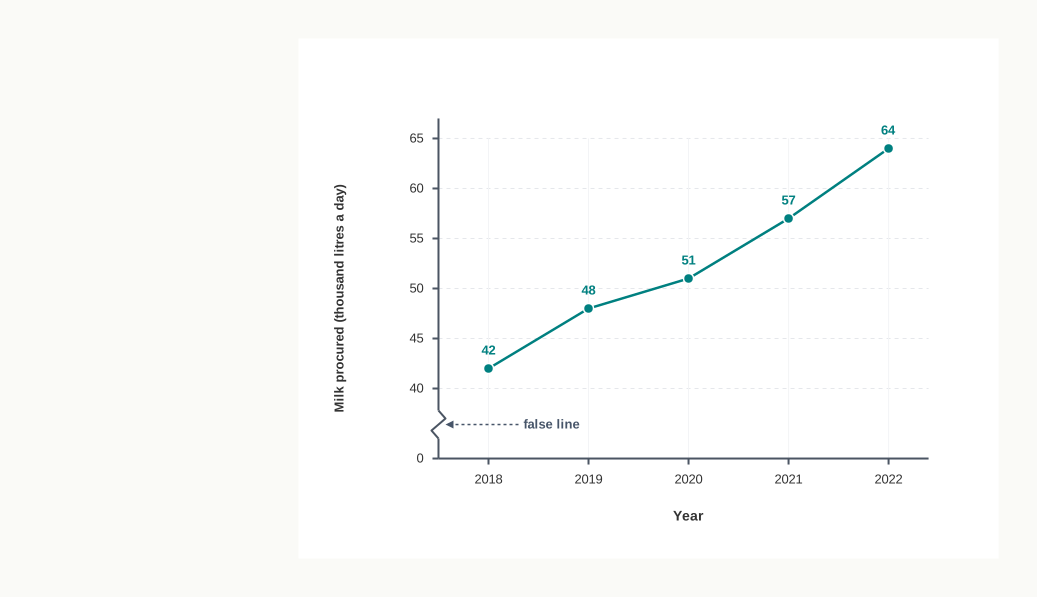
The Y-axis of Fig. 17.15 does not start at zero. Where every value in a series is large and the differences between them are small, a scale beginning at zero would compress the whole series into a narrow band near the top of the graph, and the movement would be invisible. The axis is therefore started above the origin and a false line — a cut or kink — is shown on it to warn the reader.
A false line must always be marked. An axis that begins above zero without a kink exaggerates every rise and fall, and the reader has no way of knowing it.
17.10.2.2 Two or More Variable Graphs
A two variable graph shows two or more related series on the same pair of axes, one line to each, so that their movements can be compared directly. The lines are drawn differently — one continuous, one broken — and identified by a key. Table 17.16 gives the revenue and the expenditure of a municipal body, and Fig. 17.16 plots both.
Table 17.16 — Revenue And Expenditure Of A Municipal Body, 2018 To 2022 | Year | Revenue (₹ crore) | Expenditure (₹ crore) | |—|—|—| | 2018 | 120 | 110 | | 2019 | 132 | 125 | | 2020 | 145 | 140 | | 2021 | 160 | 158 | | 2022 | 178 | 172 |
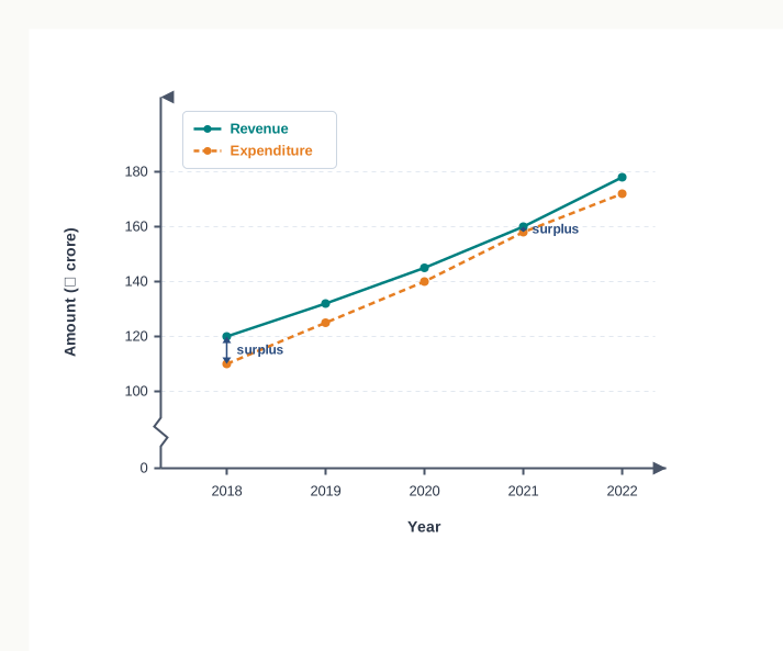
Both series rise, so a table of either alone would report growth. Only the two together show what matters, which is that the gap between them narrowed from ₹10 crore in 2018 to ₹2 crore in 2021 before widening again — the sort of relation a graph makes visible at once.
17.10.3 Frequency Line Graph
A frequency line graph is drawn for a discrete frequency distribution. The values of the variable are marked along the X-axis, and at each value a vertical line is raised whose height equals the frequency of that value.
The vertical lines stand apart and are not joined, and this is deliberate. A discrete variable takes only exact values, so there is nothing between one value and the next to plot. Fig. 17.17 draws the frequency array of household size obtained in SE 17.2.
17.10.4 Limitations of Diagrams and Graphs
Diagrams and graphs are simple, easily understood and effective at presenting data at a glance, and for time series and comparisons between groups they are the best form of presentation there is. Their limits should nevertheless be kept in view.
- They show approximations — a reader can see relative size but cannot read an exact value off a bar or a curve.
- They are of limited use where the data are numerous or the variables many, since a crowded figure is harder to read than the table it replaced.
- They can mislead — a suppressed zero, an unmarked false line or bars of unequal width all misstate the data without stating anything false in words.
- They cannot be worked upon — no average, no measure of dispersion and no correlation can be calculated from a diagram; all of these need the figures themselves.
For these reasons the figures should always accompany the picture. The two forms of presentation differ in what each is for, as set out below.
Compare Table 17.10 — Diagrammatic And Graphical Presentation | Basis | Diagrammatic Presentation | Graphical Presentation | |—|—|—| | Form used | Bars, circles and other geometric figures | Points plotted on a pair of axes and joined into a line or curve | | Material needed | Ordinary paper; drawn to a chosen scale | Graph paper, with both axes to scale | | Data suited to | Comparison between items, groups or places | Movement of a variable over time, or the relation between two variables | | What it shows best | Relative size at a glance | Direction and rate of change | | Use in further analysis | None; it is a display only | The median can be read from an ogive, and trend from a time series graph |
Reading A Price Chart Wholesale prices of an agricultural commodity are published as a monthly series and plotted as a time series graph. The table tells a trader what the price was in each month; the graph tells him whether it is climbing steadily, has flattened, or has turned. He needs both, and he acts on the second.
Distinguish the three forms by what carries the information — rows and columns in a table, the height of a bar or the angle of a sector in a diagram, and a plotted line on a pair of axes in a graph.
This completes the chapter. Data have been collected from a source by a chosen method, organised into classes and a series, and set out in a table, a diagram and a graph. What remains is to work upon them, and that is the business of the chapters that follow: to find the value about which the data centre, how widely they are spread about it, and how one series moves in relation to another.
17.11 Summary
- Data are numerical descriptions of observations relating to a group of persons, objects or events. Figures as first recorded, in no order of magnitude, are raw data; arranged by size, they become ordered data or an array.
- Data drawn from an organisation’s own records are internal data; data obtained from agencies outside it are external data.
- A statistical inquiry is a systematic process of collecting and analysing data by the use of statistical techniques. The investigator plans it, the enumerator collects in the field, and the respondent supplies the information.
- Planning an inquiry means settling three things before collection begins.
- Its objective or purpose.
- Its scope — the area, the period and the number of items to be covered.
- The population to be studied and the statistical unit in terms of which figures will be recorded.
- An inquiry passes through nine stages: planning, deciding the sources, deciding the technique, collection, processing, organisation, analysis and interpretation, preparation of the report, and its presentation.
- Data come from two sources. Primary data are collected first-hand by the investigator for the inquiry in hand; secondary data are taken from records already compiled by somebody else. The same figures are primary to the agency that collected them and secondary to everyone using them afterwards.
- Secondary data are obtained from published sources, such as government reports and the publications of international organisations, and from unpublished sources, such as the internal records of departments and research institutions. Before use they must be tested for reliability, suitability, adequacy and timeliness.
- Primary data are collected by five methods: direct personal investigation, indirect oral investigation, information from local agents and correspondents, mailed questionnaires, and questionnaires filled in by enumerators. A form filled in by the respondent is a questionnaire; the same form filled in by an enumerator is a schedule.
- A good questionnaire is short, clearly worded, logically arranged, objective and free of questions that strain the memory or invite calculation, and it is pre-tested on a small group in a pilot survey before being finalised.
- Coverage may be complete or partial. Under the census method every unit of the population is enumerated; under the sampling method only selected representative units are studied and inferences are drawn from them for the whole. The census is accurate and costly, sampling economical and open to the risk of a biased selection.
- Organisation of data is their arrangement in condensed form through classification, which divides the data into groups, and tabulation, which sets the groups out in rows and columns.
- A characteristic that can be measured is a variable; one that can only be found present or absent is an attribute. A discrete variable takes only exact values, with nothing between them; a continuous variable takes any value within a range.
- Data may be classified on four bases: place, giving geographical classification; time, giving chronological classification; attribute, giving qualitative classification, which is simple where one attribute is used and manifold where more than one is used; and numerical value, giving quantitative classification or classification by variables.
- A statistical series is data arranged in a logical order. In an individual series each item is listed singly. In a frequency series items are counted against values, the count being the frequency and the total of all frequencies being \(\sum f\).
- A discrete series or frequency array shows each exact value of a discrete variable against its frequency. A continuous series or frequency distribution groups items into classes, each with a lower limit and an upper limit, the difference between them being the class interval.
- The mid-value or class-mark of a class is the value half-way between its limits. \[m = \dfrac{l_1 + l_2}{2}\] Here \(m\) is the mid-value, \(l_1\) the lower limit and \(l_2\) the upper limit of the class, all in the units of the variable. The mid-value represents the whole class in later calculations.
- Frequency distributions take five forms.
- Exclusive, where the upper limit of a class is excluded from it and counted in the next.
- Inclusive, where all items up to and including the upper limit are counted in the class.
- Open end, where the lower limit of the first class or the upper limit of the last is missing.
- Mid-values, where only the mid-value of each class is given, the limits being recoverable by halving the difference between two consecutive mid-values and subtracting and adding it.
- Cumulative frequency, where frequencies are added progressively — downwards from the first class for a ‘less than’ series and upwards from the last for a ‘more than’ series.
- Data may be presented in three forms: in tables, in diagrams and in graphs.
- A statistical table organises data in columns and rows and has nine parts: table number, title, head note, stub head, stub entries, caption with its subheads, body of cells, footnote and source. A simple table shows one characteristic; a complex table shows two or more.
- Diagrammatic presentation sets data out as geometric figures. A simple bar diagram shows one set of figures and a multiple bar diagram two or more; a pie diagram divides a circle into sectors proportional to the shares of the components.
- The angle of a sector in a pie diagram is found as follows. \[\text{Angle of a component} = \dfrac{\text{Value of the component}}{\text{Total value}} \times 360°\] The value of the component and the total value are in the same units and the result is in degrees. Where components are given as percentages, each percentage is multiplied by 3.6, and all the angles must total 360°.
- A histogram presents a grouped frequency distribution as adjoining rectangles whose areas represent the frequencies, and is drawn only from an exclusive series. A frequency polygon joins the mid-points of the tops of those rectangles and is carried down to the axis at both ends so that its area equals that of the histogram.
- An ogive plots cumulative frequencies — a less than ogive against the upper limits, rising from left to right, and a more than ogive against the lower limits, falling from left to right. The value at which the two curves cross is the median.
- Graphical presentation plots two variables on a pair of axes, the independent variable along the X-axis. A time series graph may show one variable or several; where the scale does not begin at zero, a false line or kink must be marked on the axis. A frequency line graph shows a discrete series as separate vertical lines that are not joined.
- Diagrams and graphs convey relative size and direction of change at a glance, but they give approximations only, mislead easily if the scale is manipulated, and cannot themselves be used for calculation. The table should always accompany them.
- The three types of statistical series, which govern how every later measure is calculated, differ as follows.
Compare Table 17.11 — Individual, Discrete And Continuous Series | Basis | Individual Series | Discrete Series | Continuous Series | |—|—|—|—| | How items appear | Listed singly, each with its own value | Each exact value shown once, with its frequency | Items grouped into classes, each class with its frequency | | Frequencies | None | Present, against exact values | Present, against classes | | Variable suited to | Any, where the items are few | A discrete variable taking few values | A continuous variable, or a discrete one taking many values | | Form of presentation | Serial order or array | Frequency array of three columns | Frequency distribution with class limits | | Diagram drawn from it | None in this chapter | Frequency line graph | Histogram, frequency polygon and ogive |
17.12 Points to Ponder
- Every statistical inquiry has to choose between covering everything roughly and covering a part of it carefully. If the money available for an inquiry into household spending were halved, would you cut the number of households visited or the number of questions asked of each? What would be lost either way?
- Grouping forty marks into six classes threw away the individual figures and gave back the shape of the whole set. Is there a point at which the classes become so wide that the shape is lost as well? How would you know, working only from the data, that you had passed it?
- Secondary data cost almost nothing and cover ground no single investigator could reach, yet they were collected under somebody else’s definitions. If a set of published figures were adequate in coverage but defined ‘household’ differently from your inquiry, would you use them with a note of caution, adjust them, or collect afresh?
- A false line on an axis is honest only if the reader notices it. Two graphs of the same data, one starting at zero and one starting above it, leave different impressions of the same rise. Where does a legitimate choice of scale end and a misleading one begin?
- The census method is described as more accurate because it leaves nothing out, yet a sample can be supervised more closely, unit by unit. Under what conditions might a carefully drawn sample give a truer figure than a complete enumeration, and what does that say about the meaning of accuracy in statistics?
- Attributes such as literacy or occupation cannot be measured, only recorded as present or absent, and so cannot enter an average. Does this mean that qualitative characteristics matter less to an economist than quantitative ones, or only that they have to be studied by other means?
17.13 Objective Questions
- A researcher studying the wheat trade uses the arrivals recorded by a regulated market committee. For the researcher, these figures are [1]
- primary data, because they were collected in the field
- secondary data, because they were compiled by another agency
- primary data, because they relate to the researcher’s own subject
- neither primary nor secondary data
- In an exclusive series with the classes 20–30 and 30–40, an item of value 30 is counted in the class __________. [1]
- Assertion (A): The sampling method is preferred to the census method for testing the life of electric bulbs produced by a factory. [1] Reason (R): The census method is more costly and more time-consuming than the sampling method.
- Both A and R are true and R is the correct explanation of A
- Both A and R are true but R is not the correct explanation of A
- A is true but R is false
- A is false but R is true
- State whether the following statement is true or false, giving a reason: In a frequency line graph the vertical lines are joined to one another to form a continuous curve. [1]
- Match the items in Column I with those in Column II. [1]
| a. Chronological classification |
i. Workers grouped by daily wage into ₹300–400, ₹400–500 and so on |
| b. Manifold classification |
ii. Output of a factory shown for each year from 2018 to 2022 |
| c. Quantitative classification |
iii. Population divided by sex and each class further divided by literacy |
17.14 Check Your Concepts
- Distinguish between a questionnaire and a schedule. [2]
- Why must a false line be marked on the axis of a time series graph? Explain with reference to what a reader would otherwise conclude. [3]
- The number of members in each of twenty households of a locality was recorded as: 5, 4, 6, 4, 3, 5, 4, 7, 5, 4, 6, 3, 4, 5, 6, 4, 5, 3, 4, 6. Prepare a frequency array of the number of members, showing the tally bars, and state the value that occurs most often. [4]
- A statistical inquiry is to be conducted into the monthly expenditure of households in a town on packaged food. Explain the considerations at the planning stage, and state, with reasons, which method of collecting primary data and which technique of coverage you would recommend. [6]
17.15 Case-Based Question
- Meera Nair, who runs a small readymade garments unit, wants to know how the spending of families in her town divides between clothing and other items, so that she can plan her stock for the coming season. She has two possibilities before her. She can send a printed form by post to two thousand households across the town, asking each to record its monthly spending under six heads; or she can engage four trained assistants to visit two hundred selected households and fill in the same form by questioning the members. Her budget will stretch to only one of the two.
- Identify the method of collecting primary data in each of the two possibilities, and state one merit and one limitation of each in Meera’s situation. [2]
- Meera decides to present her findings as a pie diagram of household spending rather than as a table. State one advantage and one limitation of this choice. [2]