Chapter 20: Correlation
Every statistical measure taken up so far has looked at one variable at a time. An average tells us where a single series centres, and a measure of dispersion tells us how widely its items are scattered about that centre. Economic questions, however, involve two quantities at once. A household’s spending moves with its income. The quantity of a commodity buyers take home moves against its price. The yield of a crop moves with the rainfall of the season. In each case the interest lies not in either series by itself but in whether the two move together, in which direction, and how closely. Correlation is the statistical tool built for that question. It works on a distribution in which every item carries two values rather than one, and reduces the relationship between them to a single number stating both the direction of the association and its strength. Knowing how firmly consumption follows income, or how sharply demand follows price, allows one to be estimated from the other rather than guessed at. This chapter takes up the meaning, types and degrees of correlation, and then the three methods of measuring it — the scatter diagram, Karl Pearson’s coefficient of correlation and Spearman’s rank correlation coefficient.
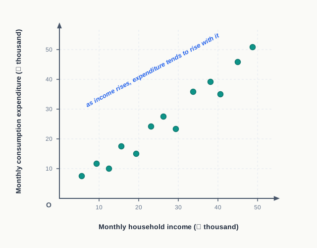
Fig. 20.0 – Scatter diagram of household income and consumption.
20.1 Studying Two Variables Together
Statistics is used in economics to reduce a mass of figures to a few readable numbers. So far that work has been done on one series at a time. An average locates the centre of a single series and a measure of dispersion states how far its items lie from that centre. Both answer questions about one variable considered on its own.
Economic questions are rarely of that kind. The interest usually lies in a pair of quantities and in whether one moves with the other. Does output rise as more fertiliser is applied? Does a firm sell more when it spends more on advertising? Does the value of a currency fall as prices within the country rise? Each of these asks about two variables at once, and no average or standard deviation can answer it.
20.1.1 Univariate and Bi-variate Distributions
A distribution in which every item carries a single value is a univariate distribution. The marks of forty students in one subject, or the daily wages of sixty workers, form such a series. All the statistical work of the earlier chapters was done on distributions of this type.
A distribution in which every item carries two values is a bi-variate distribution. Here each observation is a pair, and the pairing is what matters — the first value of one series belongs with the first value of the other, the second with the second, and so on throughout. The advertising expenditure and sales of a firm over eight years, set out in Table 20.1, form a bi-variate distribution of this kind.
Neither column in Table 20.1 is of much interest by itself. Read together, however, the two columns show that the years of heavier advertising are broadly the years of larger sales. It is this joint reading that the study of correlation makes exact.
The two forms of distribution may now be set side by side.
20.1.2 Meaning of Correlation
Two variables are said to be correlated when a change in one is accompanied by a change in the other in a regular way. If the change in the second is not regular, so that a rise in the first is sometimes met by a rise and sometimes by a fall, the two are uncorrelated.
Correlation therefore records an association, and that association has two aspects. The first is direction — whether the two variables move the same way or opposite ways. The second is degree — how closely the movement of one is matched by the movement of the other. A measure of correlation states both in a single number.
20.1.3 Significance of Correlation
The value of the tool lies in what it allows the economist to do once the association is known.
- It measures the strength of a relationship — the closeness of two series is reduced to one number that can be compared across pairs of variables and across periods, which no eye-reading of two columns of figures can supply.
- It supports estimation — where income and consumption are known to be closely correlated, the consumption of a household can be estimated from its income with reasonable confidence instead of being guessed at.
- It tests economic theory — the law of demand asserts an inverse relation between price and quantity demanded, and correlation measured from market data shows whether the figures bear the assertion out.
- It guides policy and business decisions — a firm that knows how closely its sales follow its advertising can judge whether further expenditure is worth undertaking.
- It narrows a field of enquiry — a high correlation between two variables marks the pair as worth investigating for a causal link, and a very low one suggests that the search should be directed elsewhere.
The last point needs care. Correlation establishes association, not causation. Where two variables are found to move together, the relationship may run from the first to the second, from the second to the first, or from a third variable acting on both. It may also be the outcome of chance alone. Deciding which of these holds is a matter for economic reasoning about the variables concerned, and the statistical measure cannot settle it.
20.2 Types of Correlation
Once two variables are known to be associated, the association has to be described before it can be measured. Correlation is classified on three counts — the direction in which the two variables move, the steadiness of the ratio in which they move, and the number of variables brought into the study at one time.
20.2.1 Positive and Negative Correlation
Classification by direction is the first and the most used. Two variables are positively correlated when they move in the same direction, and negatively correlated when they move in opposite directions.
Positive correlation exists where a rise in one variable is accompanied by a rise in the other, and a fall by a fall. The relation between the number of workers employed in a factory and its total output, shown in Table 20.2, is of this kind.
Negative correlation exists where the two variables move in opposite directions, a rise in one being accompanied by a fall in the other. Sales of woollen garments against the average temperature of the month, set out in Table 20.3, follow this pattern.
The direction of correlation is carried by the sign of the coefficient. A positive sign records movement in the same direction and a negative sign movement in opposite directions. The sign says nothing about how close the relationship is; that is a separate matter, taken up in the next section. The two directions may be set against each other as follows.
20.2.2 Linear and Non-linear Correlation
The second classification looks not at the direction of the movement but at its steadiness.
Correlation is linear when a change in one variable is met by a change in the other in a constant ratio throughout the series. If every addition of one worker raises output by twenty units, whether the tenth worker or the twentieth, the ratio holds constant and the correlation is linear. Plotted on a graph, such a pair of series yields points that lie on or about a straight line.
Correlation is non-linear when the ratio does not stay constant. Here a change in one variable is still accompanied by a change in the other, but the size of the response varies from one part of the series to another. Output may rise steeply as the first few workers are added and only slightly as later ones are taken on. Plotted on a graph, the points trace a curve rather than a straight line. The two patterns are compared in Fig. 20.1.
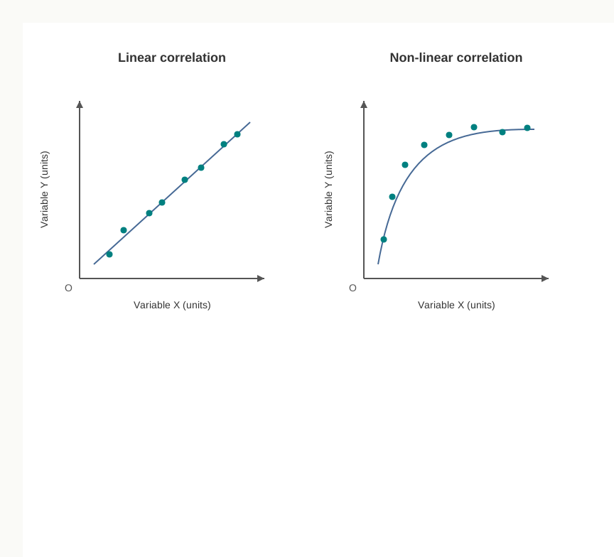
Fig. 20.1 – Linear and non-linear correlation.
Most relationships in economics are non-linear in strict terms. The methods prescribed at this stage nevertheless assume a linear relationship, because a straight line is a serviceable approximation over the range of values ordinarily observed and keeps the arithmetic within reach.
20.2.3 Simple, Multiple and Partial Correlation
The third classification rests on the number of variables under study.
- Simple correlation — the relationship between two variables only, such as the price of a commodity and the quantity of it supplied. All the measurement taught in this chapter is of this type.
- Multiple correlation — the relationship between one variable and two or more others taken together, such as the milk yield of a herd studied against feed, breed and veterinary care at the same time.
- Partial correlation — the relationship between two variables while the remaining variables are held constant, such as the relation of milk yield to feed alone, with breed and veterinary care treated as unchanged.
Multiple and partial correlation are noted here for their meaning alone. Their measurement lies outside the scope of this course, and every method that follows is applied to two variables only.
20.3 Degrees of Correlation
Direction answers only half the question. Two pairs of variables may both move in the same direction and yet differ greatly in how faithfully the second follows the first. The degree of correlation is the second aspect of the association, and it states how close that following is.
20.3.1 The Coefficient of Correlation as a Measure of Degree
Both aspects of correlation are carried by a single figure, the coefficient of correlation. It is written as \(r\) when computed by Karl Pearson’s method and as \(r_k\) when computed from ranks, and it is a pure number, free of the units in which either variable is measured.
The coefficient cannot fall outside a fixed range.
\[-1 \leq r \leq +1\]
Here \(r\) is the coefficient of correlation, \(-1\) its lowest possible value and \(+1\) its highest. The sign of \(r\) gives the direction of the relationship and its numerical size, read without the sign, gives the degree. The nearer the figure lies to either end of the range, the closer the relationship; the nearer it lies to the middle, the looser. This range is shown in Fig. 20.2.
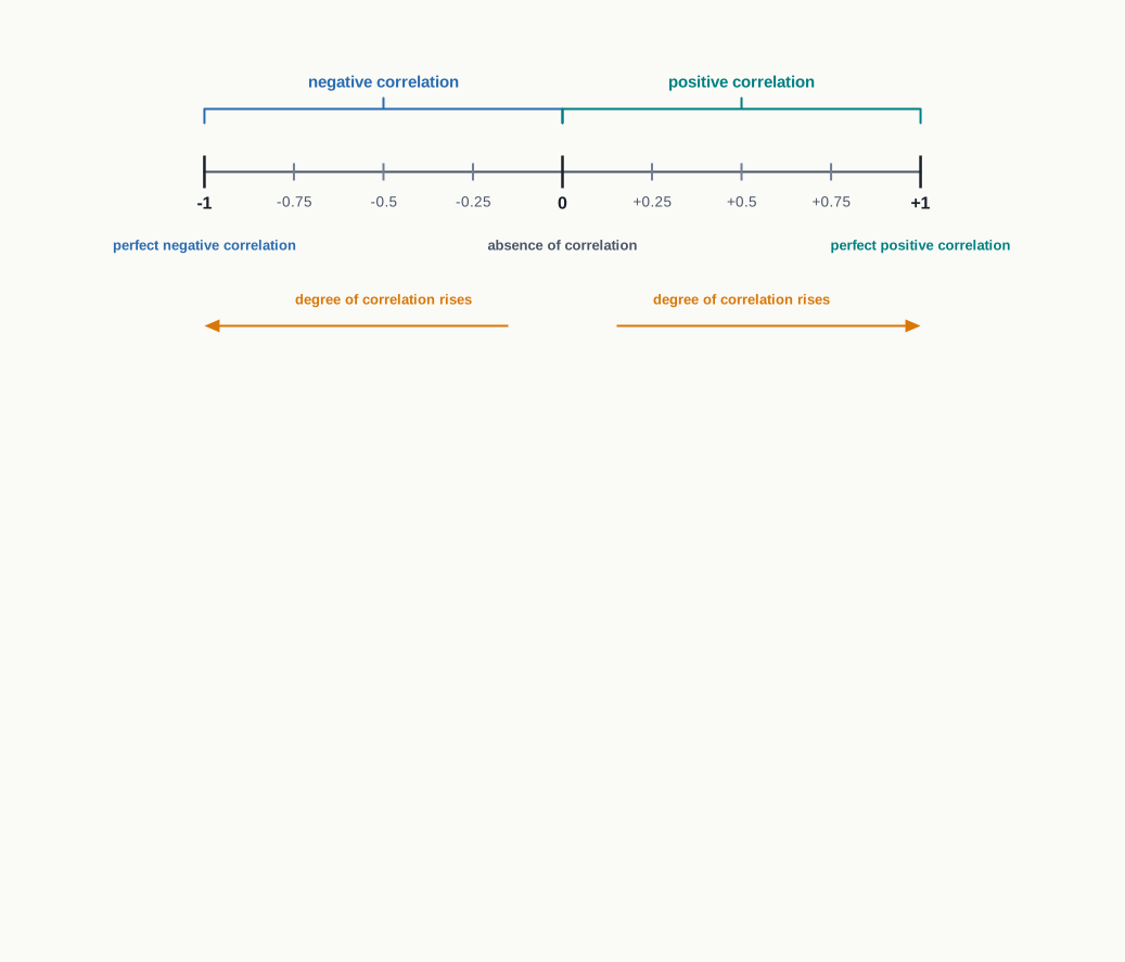
Fig. 20.2 – The range of the coefficient of correlation.
20.3.2 Perfect Correlation
Correlation is perfect when the two variables move in a constant ratio throughout the series, so that the change in one is matched exactly by a proportionate change in the other at every point. The coefficient then takes one of the two extreme values of its range.
- Perfect positive correlation — the two variables move in the same direction in a constant ratio, and \(r = +1\). If a worker paid a fixed rate per piece produces twice as many pieces, the wage earned is exactly doubled.
- Perfect negative correlation — the two variables move in opposite directions in a constant ratio, and \(r = -1\). If a fixed sum is divided between two heads of expenditure, every rupee added to the first is a rupee taken from the second.
Perfect correlation is common enough where one variable is defined in terms of the other by an arithmetical rule. It is almost never found in economic data drawn from observation, because any real pair of variables is disturbed by other influences that no rule accounts for.
20.3.3 Absence of Correlation
Correlation is absent when a change in one variable is not accompanied by any regular change in the other. A rise in the first is met sometimes by a rise and sometimes by a fall in the second, with no pattern running through the series, and the coefficient works out to \(r = 0\).
The height of a group of workers and the wages they earn is a pair of this kind. The two figures can be collected and set alongside each other, but no relationship exists between them and none appears in the coefficient. Where \(r = 0\) the two variables are said to be uncorrelated. The two extremes of the range may be compared with this middle case as follows.
20.3.4 Limited Degrees of Correlation
Between the extremes and the middle lie the values actually met with in practice. These are the limited degrees, and they are described by how near the coefficient stands to 1, its sign being set aside for the purpose. The customary description is given in Table 20.4.
These bands are a convention adopted for convenience of description and not a rule of measurement. Nothing changes in the arithmetic as a coefficient passes from 0.74 to 0.76; only the word used to report it changes. The figure itself, with its sign, remains the statement of the result, and the description is added to make that figure readable.
20.4 Methods of Measuring Correlation
Direction and degree have now been described. What remains is to obtain them from the figures themselves. Three methods are prescribed for the purpose — the scatter diagram, Karl Pearson’s coefficient of correlation and Spearman’s rank correlation coefficient. Each works on a bi-variate distribution and each ends in a statement about direction and degree, but they differ in the form of the data they need and in the exactness of the answer they give.
The Graphic Method
The scatter diagram plots the paired values as points on a graph and leaves the relationship to be read from the pattern the points form. It is quick, needs no arithmetic and shows at a glance whether the association is positive or negative and whether it is close or loose. What it does not give is a number. Two scatters may both look close without the diagram settling which of them is the closer, and a diagram cannot be carried into any further calculation.
The Algebraic Methods
The two algebraic methods answer with a coefficient.
Karl Pearson’s coefficient works on the values themselves. It compares the deviations of each variable from its own mean and yields the most exact measure of the three, but it requires the data to be quantitative and it assumes the relationship to be linear.
Spearman’s rank correlation works on the ranks of the values rather than the values. Its exactness is lower, since the ranks discard the size of the gaps between the items, but it can be applied where Karl Pearson’s method cannot — to qualities that can be ordered but not measured, and to series carrying items so extreme that the mean is pulled out of position.
Choosing A Method
The choice among the three follows from the data in hand and the use the answer is to be put to. The main points of difference are set out below.
In practice the scatter diagram is drawn first and the coefficient computed afterwards. The diagram warns whether the relationship is linear, which is the condition Karl Pearson’s method assumes; where the points trace a curve, a coefficient computed from them will understate a relationship that plainly exists.
Each method is taken up in turn in the sections that follow — the scatter diagram in 20.5, Karl Pearson’s coefficient in 20.6 and Spearman’s rank correlation in 20.7.
20.5 The Scatter Diagram
The simplest of the three methods puts the figures on a graph and lets the relationship show itself. Nothing is computed. The pairs are plotted as points and the pattern the points form is read for direction and degree.
20.5.1 Meaning and Construction of a Scatter Diagram
A scatter diagram is a graph on which each pair of values in a bi-variate distribution is shown as a single point. One variable is taken on the X-axis and the other on the Y-axis, and a point is marked where the two values of a pair meet. A distribution of eight pairs yields eight points, and the cluster they form is the scatter.
The steps in drawing one are few.
- Choose the axes — the variable treated as the influencing one is taken on the X-axis and the other on the Y-axis, each labelled with its unit.
- Fix the scales — the scale on each axis is chosen so that the whole range of that variable fits the space available, and the two scales need not be the same.
- Plot the pairs — for each pair, move along the X-axis to the value of the first variable and up to the value of the second, and mark a dot where the two meet.
- Read the scatter — examine the direction in which the cluster of dots runs and how tightly the dots are packed about that direction.
The figures in Table 20.5, giving the number of retail outlets a beverage company maintains in eight towns and its monthly sales in each, are plotted in this way in Fig. 20.3.
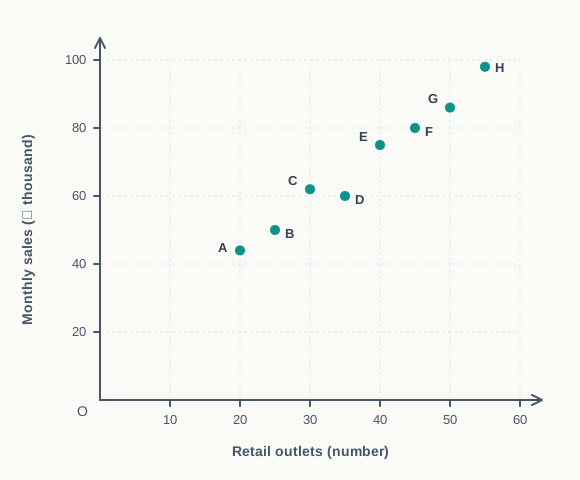
Fig. 20.3 – Scatter diagram of retail outlets and monthly sales.
20.5.2 Reading Direction and Degree from the Scatter
The scatter is read on the two counts already familiar. Direction is given by the way the cluster runs, and degree by how tightly the dots hold to that run.
Direction Of The Scatter
Where the dots run upward from the lower left to the upper right, the two variables rise and fall together and the correlation is positive. Where they run downward from the upper left to the lower right, one rises as the other falls and the correlation is negative. Where they show no drift in either direction, no correlation is present.
Degree Of The Scatter
Degree is judged by the width of the band the dots occupy. Dots lying exactly on a single straight line show perfect correlation. As the band widens the degree falls, and dots spread evenly over the whole space show the absence of correlation. The two perfect cases are drawn in Fig. 20.4.
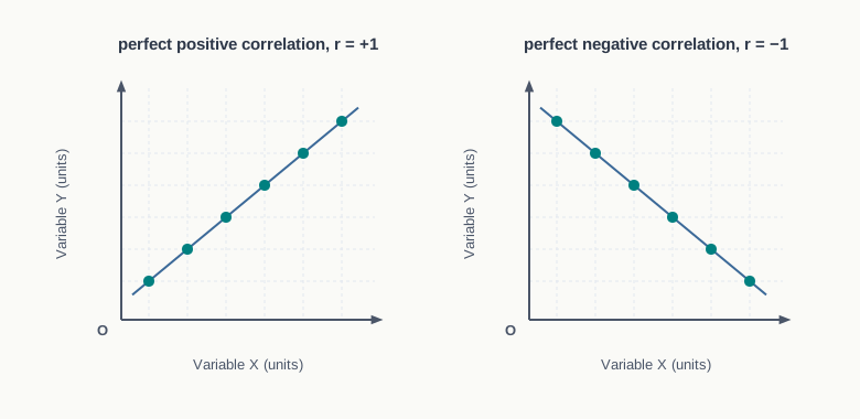
Fig. 20.4 – Perfect positive and perfect negative correlation.
The cases met with in practice lie between these extremes, and three of them are shown in Fig. 20.5.
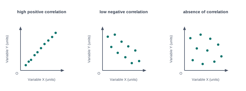
Fig. 20.5 – Limited degrees and the absence of correlation.
20.5.3 Merits and Demerits of the Scatter Diagram
The method is worth using for what it does quickly, and worth leaving for what it cannot do at all.
Merits
- Simplicity — the diagram needs no computation and no knowledge of any formula, and can be drawn as soon as the paired values are in hand.
- Immediate reading — direction and rough degree are taken in at a glance, which no table of figures allows.
- Detection of non-linearity — a scatter tracing a curve shows at once that the relationship is not linear, a warning no coefficient carries.
- Independence from extreme items — a single unusually large or small pair stands out as a stray dot and does not distort the pattern the rest of the dots make.
- A guide to further work — the diagram shows whether measurement is worth undertaking and which method it should be undertaken by.
Demerits
- No numerical result — the method gives no coefficient, so the degree of correlation cannot be stated exactly or compared with that of another pair of variables.
- Dependence on judgement — the reading rests on the eye of the reader, and two people may describe the same scatter differently.
- No use in further calculation — a pattern of dots cannot be carried into any later statistical work, as a coefficient can.
- Unsuitability for large distributions — a distribution running to hundreds of pairs produces a crowd of dots from which no clear band can be read.
20.6 Karl Pearson’s Coefficient of Correlation
The scatter diagram shows a relationship but does not measure it. Karl Pearson’s method supplies the measurement. It works on the values themselves and reduces the whole bi-variate distribution to one figure carrying both direction and degree.
20.6.1 Meaning of the Coefficient of Correlation
The method rests on a simple idea. If two variables are related, then the items standing above the mean of the first series should tend to stand above the mean of the second as well, and the items standing below one mean should tend to stand below the other. The method therefore works not with the values but with their deviations from their own means, and asks how regularly the two sets of deviations agree in sign and in size.
The method carries three assumptions, and each of them limits where it may be used.
- The relationship is linear — the two variables are taken to change in a constant ratio, so the coefficient understates a relationship that traces a curve.
- A cause-and-effect relation exists between the variables — the method is meant for pairs that can sensibly be connected, and applying it to unconnected series yields a figure that means nothing.
- The variables are affected by a large number of independent causes — the many small influences at work are taken to offset one another, so that the pattern left in the data is the relationship being measured.
20.6.2 The Direct Method
The direct method takes deviations from the actual arithmetic mean of each series. It is used where both means work out to whole numbers, since deviations from a fractional mean turn the arithmetic awkward.
The coefficient compares the sum of the products of the paired deviations with the spread of the two series taken together, so that a close agreement of deviations yields a large value and an irregular one a small value.
\[r = \dfrac{\sum xy}{\sqrt{\sum x^2 \times \sum y^2}}\]
Here \(x = X - \bar{X}\) is the deviation of an item of the first series from its mean and \(y = Y - \bar{Y}\) the deviation of the corresponding item of the second series from its mean; \(\sum xy\) is the total of the products of the paired deviations, and \(\sum x^2\) and \(\sum y^2\) the totals of their squares. The result is a pure number lying between −1 and +1, read for direction by its sign and for degree by its size.
The steps are four. The two means are found; the deviations \(x\) and \(y\) are taken; the columns \(xy\), \(x^2\) and \(y^2\) are worked out and totalled; and the totals are placed in the formula. The arrangement is shown in SE 20.1, for which the working is set out in Table 20.6.
20.6.3 The Short-cut Method
Where the means are fractional, deviations from them run into decimals and the squaring becomes laborious. The short-cut method avoids this by taking deviations from an assumed mean — any convenient value chosen from within the series — and then correcting the result for the difference between the assumed mean and the actual one.
\[r = \dfrac{\sum dx\,dy - \dfrac{\sum dx \times \sum dy}{N}}{\sqrt{\sum dx^2 - \dfrac{(\sum dx)^2}{N}} \times \sqrt{\sum dy^2 - \dfrac{(\sum dy)^2}{N}}}\]
Here \(dx = X - A_x\) and \(dy = Y - A_y\) are the deviations of the two series from their assumed means \(A_x\) and \(A_y\), \(N\) is the number of pairs, and \(\sum dx\,dy\), \(\sum dx^2\) and \(\sum dy^2\) are the totals of the product and square columns. The three terms subtracted are the corrections for the assumed means. The result is read exactly as before, and it is the same figure the direct method would give on the same data.
The method is set out in SE 20.2, with the working in Table 20.7.
The short-cut method comes into its own where the figures themselves are large, since the assumed mean may be placed near the centre of the series and the deviations kept small. SE 20.3 is of that kind, with its working in Table 20.8.
20.6.4 Interpreting the Value of the Coefficient
A computed coefficient is not an answer until it has been read. Four properties govern the reading.
- The coefficient lies between −1 and +1 — a value outside this range can only mean an arithmetical error, and the working should be checked rather than the result reported.
- The sign gives the direction — a positive coefficient records movement in the same direction and a negative one movement in opposite directions.
- The size gives the degree — the sign is set aside and the figure read against the bands of Table 20.4, so that 0.9 and −0.9 stand for equally close relationships.
- The coefficient is a pure number — it carries no unit and is unaffected by the units in which the two variables are measured, so income in rupees against output in quintals yields the same coefficient as income in thousands of rupees against output in tonnes.
The reading is completed in words. A coefficient of +0.98 between area and output is reported not as a number alone but as a high degree of positive correlation, meaning that farms with larger areas under the crop are, in this data, the farms with larger output.
20.6.5 Merits and Demerits of Karl Pearson’s Method
Merits
- Exactness — the method gives a single definite figure, so the relationship can be stated precisely and compared with that between any other pair of variables.
- Direction and degree together — one coefficient carries both, the sign supplying the first and the size the second.
- Independence of units — being a pure number, the coefficient allows series measured in different units to be compared directly.
- Use of the whole data — every pair of values enters the computation, so nothing observed is discarded.
- A basis for further work — the coefficient can be carried into later statistical analysis, which a diagram cannot.
Demerits
- Assumption of linearity — the method takes the relationship to be linear and understates a close relationship that traces a curve.
- Sensitivity to extreme items — the deviations are squared, so one unusually large or small pair can move the coefficient appreciably.
- Length of computation — the method is the most laborious of the three, particularly where the means are fractional.
- Restriction to quantitative data — qualities that can be ordered but not measured, such as beauty or honesty, cannot be handled at all.
- Risk of misreading — a high coefficient is easily taken for proof of causation, which the method does not supply.
20.7 Spearman’s Rank Correlation Coefficient
Karl Pearson’s method needs measured values. A great deal of the material an economist works with cannot be measured at all, and some of what can be measured carries items so extreme that the mean is dragged out of position. For both cases there is a second algebraic method, which works on the order of the items instead of their values.
20.7.1 Why Ranks Are Used
Ranking arranges the items of a series in order — first, second, third — without recording how far apart they stand. That loss of information is the price of the method, and it buys two things Karl Pearson’s method cannot supply.
- Qualities can be handled — honesty, efficiency, consumer preference and the quality of a product have no unit and cannot be added or averaged, but a set of items can be placed in order on any of them, and ranks so obtained can be correlated.
- Extreme items are contained — a single very large value takes only the first rank, however large it is, so it cannot pull the result about as it does when squared deviations from the mean are used.
The coefficient obtained is written \(r_k\) and is read exactly as \(r\) is read, lying between −1 and +1 and carrying direction in its sign and degree in its size.
The coefficient rests on the differences between the paired ranks. Where the two orders agree at every place, every difference is zero and the coefficient reaches +1; where the orders are exactly reversed, the differences are at their largest and the coefficient reaches −1.
\[r_k = 1 - \dfrac{6\sum D^2}{N^3 - N}\]
Here \(D\) is the difference between the two ranks of a pair, \(\sum D^2\) the total of the squares of those differences and \(N\) the number of pairs. The 6 in the numerator is a constant of the formula and is not to be altered. The result is a pure number between −1 and +1.
20.7.2 When Ranks Are Given
Where the data already comes as ranks, no ranking is needed and the work begins at the difference column. The differences are taken pair by pair, squared and totalled, and the total placed in the formula. The arrangement is shown in SE 20.4, with the working in Table 20.9.
20.7.3 When Ranks Are Not Given
Where the data comes as values, the values must first be ranked. Each series is ranked separately and within itself, the largest item taking rank 1, the next rank 2, and so on to the smallest. The order chosen must be the same for both series — if the largest is ranked first in one, it must be ranked first in the other as well, or the sign of the result is reversed. Once the ranks are in place the work proceeds as before, as SE 20.5 shows, with the working in Table 20.10.
20.7.4 When Ranks Are Equal
Two or more items of a series are sometimes equal in value, and no reason exists for placing one above the other. Such items are given the same rank, taken as the average of the ranks they would have occupied between them. Two items competing for the third and fourth places each take rank 3.5; three items competing for the second, third and fourth places each take rank 3.
Equal ranks disturb the formula, because the ranks of the series no longer run as a plain sequence. A correction is therefore added to \(\sum D^2\) for every group of tied items.
\[r_k = 1 - \dfrac{6\left[\sum D^2 + \dfrac{1}{12}(m_1^3 - m_1) + \dfrac{1}{12}(m_2^3 - m_2) + \cdots\right]}{N^3 - N}\]
Here \(m_1\), \(m_2\) and so on are the numbers of items in each group of equal ranks, one such term being added for every group in either series, and \(N\) is the number of pairs. Where an item ties with one other, \(m = 2\) and the term works out to 0.5. The method is shown in SE 20.6, with the working in Table 20.11.
20.7.5 Merits and Demerits of Rank Correlation
Merits
- Application to qualities — attributes that can be ordered but not measured are brought within the reach of correlation, which no other method allows.
- Simplicity — the arithmetic is shorter than Karl Pearson’s, and once the ranks are in place only one column has to be squared and totalled.
- Resistance to extreme items — an unusually large or small value takes only the first or the last rank, so it cannot distort the result.
- Use with incomplete data — where the values themselves are not known but the order is, the method still yields a coefficient.
Demerits
- Loss of information — the size of the gaps between items is discarded, so two series that differ greatly in spread give the same ranks and the same coefficient.
- Lower exactness — being computed from ranks, the coefficient is an approximation to the one Karl Pearson’s method would give on the same data.
- Labour with large distributions — ranking becomes long and error-prone as the number of items rises.
- Unsuitability for grouped data — the method is applied to individual items in pairs and cannot be used on a frequency distribution.
20.8 Summary
- Averages and measures of dispersion describe one variable at a time. Correlation is the tool used where each item carries two values and the question is whether the two variables move together.
- A univariate distribution records one value for each item; a bi-variate distribution records two, and the pairing of the values is what makes the study of correlation possible.
- Correlation states two things about a relationship:
- Direction — whether the two variables move the same way or opposite ways.
- Degree — how closely the movement of one is matched by the movement of the other.
- Correlation shows association only. It does not establish that one variable causes the other, since the relation may run either way, may arise from a third variable acting on both, or may be the outcome of chance, in which case it is called spurious correlation.
- Correlation is classified on three bases:
- Direction of movement — positive, where both variables move the same way, and negative, where they move opposite ways.
- Ratio of change — linear, where the ratio stays constant and the points fall about a straight line, and non-linear, where the ratio varies and the points trace a curve.
- Number of variables — simple for two variables, multiple for one variable against two or more together, and partial for two variables with the rest held constant.
- The coefficient of correlation is a pure number confined to a fixed range, \(-1 \leq r \leq +1\), where \(r\) is the coefficient. Its sign gives the direction of the relationship and its size, read without the sign, gives the degree.
- Correlation is perfect at \(r = +1\) or \(r = -1\), where the two variables move in a constant ratio, and absent at \(r = 0\), where no regular movement links them. Values between are described as high, moderate or low by convention, not by any rule of measurement.
- Three methods of measurement are prescribed — the scatter diagram, Karl Pearson’s coefficient of correlation and Spearman’s rank correlation coefficient.
- The scatter diagram plots each pair as a point and leaves the relationship to be read from the pattern. A band running upward from the lower left shows positive correlation and one running downward shows negative correlation; the narrower the band, the higher the degree. It is quick and shows non-linearity at once, but yields no number and cannot be carried into further work.
- Karl Pearson’s coefficient measures linear correlation from the deviations of each series about its own mean. By the direct method, using deviations from the actual means: \[r = \dfrac{\sum xy}{\sqrt{\sum x^2 \times \sum y^2}}\] Here \(x = X - \bar{X}\) and \(y = Y - \bar{Y}\) are the deviations of a pair from their respective means, \(\sum xy\) is the total of their products, and \(\sum x^2\) and \(\sum y^2\) the totals of their squares.
- Where the means are fractional, deviations are taken from assumed means and the short-cut method is used: \[r = \dfrac{\sum dx\,dy - \dfrac{\sum dx \times \sum dy}{N}}{\sqrt{\sum dx^2 - \dfrac{(\sum dx)^2}{N}} \times \sqrt{\sum dy^2 - \dfrac{(\sum dy)^2}{N}}}\] Here \(dx = X - A_x\) and \(dy = Y - A_y\) are deviations from the assumed means \(A_x\) and \(A_y\), and \(N\) is the number of pairs. The choice of assumed mean does not affect the result.
- Karl Pearson’s method assumes a linear relationship, a sensible cause-and-effect connection between the variables, and the presence of many independent influences. It is the most exact of the three methods, but it needs quantitative data and is disturbed by extreme items.
- Spearman’s method works on the order of the items rather than their values, and so reaches qualities that cannot be measured and resists extreme items: \[r_k = 1 - \dfrac{6\sum D^2}{N^3 - N}\] Here \(D\) is the difference between the two ranks of a pair, \(\sum D^2\) the total of the squares of those differences and \(N\) the number of pairs.
- Where two or more items of a series are equal, each is given the average of the ranks they would have occupied, and a correction is added for every such group: \[r_k = 1 - \dfrac{6\left[\sum D^2 + \dfrac{1}{12}(m_1^3 - m_1) + \dfrac{1}{12}(m_2^3 - m_2) + \cdots\right]}{N^3 - N}\] Here \(m_1\), \(m_2\) and so on are the numbers of items in each group of equal ranks, one term being added for each group in either series.
- Both series must be ranked in the same order, and the differences must total zero. A non-zero \(\sum D\) signals an error in ranking.
- The two algebraic methods answer the same question from different data, and differ as follows.
- Whichever method is used, the answer is complete only when read in words — the sign reported as the direction of the relationship and the size as its degree, with no claim of causation attached.
20.9 Points to Ponder
A study finds a high positive correlation between the number of hospitals in a district and the number of recorded illnesses. Does the figure suggest that hospitals make people ill, that illness draws hospitals to a district, or that some third condition explains both? What would you need to know before deciding?
Karl Pearson’s method assumes a cause-and-effect relation between the two variables, yet the coefficient can be computed from any two series of the same length, however unconnected. If the arithmetic never objects, what protects a study from producing meaningless results?
Spearman’s method discards the size of the gaps between items and keeps only their order. Two districts may be separated by a wide gap in per capita income and two others by a narrow one, and both pairs count the same once ranked. When is this loss a reasonable price to pay, and when does it hide something the economist needed to see?
Economic relationships are seldom linear — the response of output to fertiliser, or of consumption to income, usually weakens as the quantity rises. The methods taught here assume linearity all the same. Is a straight-line measure of a curved relationship a useful approximation or a misleading one?
The bands describing a coefficient as high, moderate or low are a convention rather than a rule. A study reporting a coefficient of 0.76 may describe its result as a high degree of correlation while another reporting 0.74 calls its own moderate. What difficulties does this create when findings from different studies are compared?
Suppose a firm establishes that its sales are highly correlated with its advertising expenditure over the past ten years. How far can that finding be relied on in deciding next year’s advertising budget, and what could make the relationship break down?
20.10 Objective Questions
- The coefficient of correlation between two variables works out to −1.2. This means that: [1]
- the two variables are perfectly negatively correlated
- the two variables are uncorrelated
- an error has been made in the computation
- the relationship between the two variables is non-linear
- Assertion (A): A coefficient of correlation of zero between two variables does not prove that the two are unrelated. [1] Reason (R): Karl Pearson’s coefficient measures linear correlation only, and a relationship that traces a curve may yield a coefficient of zero.
- Both A and R are true and R is the correct explanation of A.
- Both A and R are true but R is not the correct explanation of A.
- A is true but R is false.
- A is false but R is true.
- Where two items of a series are equal in value, each is given the __________ of the ranks they would have occupied. [1]
- State whether the following is true or false, with a reason: The scatter diagram gives the exact degree of correlation between two variables. [1]
- Match the descriptions in Column A with the terms in Column B: [1]
| Column A | Column B |
|---|---|
| a. Two variables move in opposite directions | i. Linear correlation |
| b. One variable is studied against two others taken together | ii. Negative correlation |
| c. A change in one variable is met by a change in the other in a constant ratio | iii. Multiple correlation |
20.11 Check Your Concepts
- Define correlation and state the two things a coefficient of correlation tells us about a relationship. [2]
- Distinguish between positive and negative correlation, giving one economic example of each. [3]
- ‘A high coefficient of correlation between two variables proves that one causes the other.’ Evaluate this claim, supporting your answer with an example. [4]
- The following figures give the number of tube wells and the area irrigated on five farms. Calculate Karl Pearson’s coefficient of correlation by the direct method and state the direction and degree of the relationship. [6] Tube wells: 3, 6, 9, 12, 15 Area irrigated (hectares): 10, 14, 20, 24, 32
20.12 Case-Based Question
- Rohit Sen runs a stationery shop and has begun offering a discount during the school admission season. Over six weeks he records the discount offered as a percentage of the marked price and the number of notebooks sold in that week. Plotting the pairs, he finds the dots running upward from the lower left to the upper right in a narrow band. In the same six weeks he also notes the ranks his three suppliers are given by his customers for quality and the ranks he himself gives them for price. [4]
- State what Rohit’s plotted diagram is called, and what its pattern tells him about the direction and degree of the relationship between discount and notebooks sold. [2]
- Rohit wishes to measure the relationship between the quality ranks and the price ranks of his three suppliers. Name the method he should use and give one reason why Karl Pearson’s method would not serve. [2]