Chapter 18: Measures of Central Value

Numbers arrive in bulk. The marks of four hundred candidates in a board examination, the rainfall recorded at fifty stations through a monsoon, the electricity bill of every household on a street — data of this kind cannot be held in the mind, and it cannot be compared. Classifying and tabulating the figures is only the first step. They must be condensed further, until the whole set can be spoken of in a single value. That value is called a central value, or an average. It is one number, drawn from within the range of the data, chosen to stand for all of them. Say that the candidates of one school averaged 90 marks and those of another 95, and a comparison that was impossible a moment earlier becomes immediate. Economics rests on averages constantly — average income, average cost, average output — so a careful question follows. Which single value truly represents a series, and how is it to be computed from the data actually in hand? This chapter takes up the three averages the syllabus prescribes: the arithmetic mean, the median and the mode. It works each of them out for individual, discrete and continuous series, adds the weighted mean, locates the median and the mode graphically, and closes with the relationship among the three and the grounds for choosing between them.

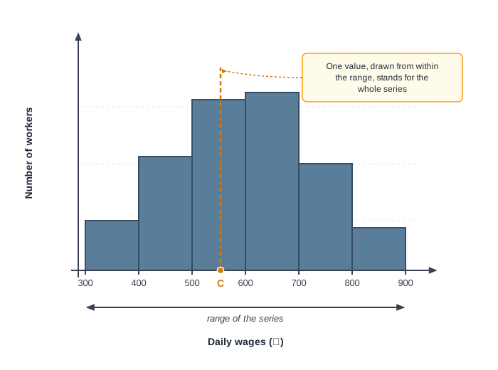
Fig. 18.0 – A series and its central value.

18.1 The Idea of an Average

18.1.1 Why Raw Data Must Be Summarised

The purpose of statistical analysis is to make a mass of information intelligible. Data as first collected are raw — a long list of figures in no particular order, carrying no meaning that can be read off at a glance. Before anything can be said about them, they must be reduced to a manageable form.

Classification is the first step in that reduction. Sorting the figures into classes and arranging them in a table brings out the main characteristics of the data and shows how the observations are distributed. But classification only organises the information; it does not shrink it.

Even a well-drawn frequency table may run to many rows, and a reader who wants to compare one set of data with another still has too much to hold in mind. The data must therefore be condensed a second time, until the characteristic of the whole set is expressed in one single value.

That single value is called a central value, or an average. It is the number the series can be spoken of by, and it is what makes comparison between two series possible at all.

Economy Example

Per Capita Income Is An Average India’s per capita income is national income divided by the total population — a single figure standing for the income of every resident. It condenses the earnings of more than a billion people into one number, which is why it is used to compare India with other economies. It says nothing, however, about how unequally that income is actually shared.

18.1.2 Average Defined

An average is a single value that is representative of all the items in a series. Because the individual values of a series usually cluster around it, an average is also called a measure of central tendency — it marks the centre about which the observations tend to gather.

Two features are essential to the idea. First, the average must lie within the range of the data, somewhere between the smallest and the largest item. Second, it must be used to represent all the values of the series, not merely a few of them.

Definition

Average An average is a single value within the range of the data that is used to represent all the values in the series. Since it lies somewhere within the central range of the data, it is also called a measure of central value. It expresses the characteristic of the whole series in one figure.

The word is familiar from ordinary speech long before it is met in statistics. Average rainfall, average height, average yield of milk per cow, average size of a family — in every case a single value is being offered as the representative of many.

Measures of central tendency are the methods of statistical analysis by which such a value is estimated. Their standing in the subject is such that Bowley described statistics as the science of averages.

18.1.3 Objectives of Studying Averages

An average is computed for definite purposes, and knowing what those purposes are helps in judging whether a particular average has served them. Three objectives are usually stated.

Representation of the data — the first aim is to arrive at a single figure for the whole series that may be used in place of it. All later use of the average depends on how faithfully that one figure stands for the many.
Description of the basic feature — the average gives a bird’s-eye view of the data and describes the characteristic of the entire group. It would be meaningless to recite the height of every student in a school, but the average height tells us at once whether the students are tall or short.
Facilitating comparison — averages allow one set of data to be set beside another. The output of two factories, the yield of two districts or the performance of two sections of a class can be compared only after each has been reduced to a single representative value.

Exam Pointer

When a question asks you to define an average, give the definition in the subject’s own words — ‘a single value within the range of the data used to represent all the values in the series’. Answers that say only ‘the middle value’ lose the mark.

18.1.4 Characteristics of a Good Average

Since several different averages exist, some standard is needed against which each may be judged. A good average should satisfy the following characteristics.

Rigidly defined — the average should be defined properly and clearly, so that its value is fixed by the data and leaves no scope for misunderstanding or differing interpretation.
Based on all the items — it should take every item of the series into account, since a value drawn from only part of the data cannot represent the entire mass of it.
Simple to calculate — a measure that is easy to compute will be widely used, while one that demands elaborate working will not be, whatever its other merits.
Easy to understand — the average should be readily understood by a person of ordinary intelligence, because it is meant to communicate the character of the data to others.
Least affected by extreme observations — one or two unusually small or unusually large items should not pull the average away from the bulk of the data, or it ceases to represent the series.
Capable of algebraic treatment — an average that can be handled mathematically is of greater practical use. If the average income of two groups and the size of each group are known, it should be possible to work out their combined average income.
Sampling stability — the average should be least affected by fluctuations of sampling. If four different groups are drawn from the same class to find the average height of its students, the four results should not differ materially from one another.

No single average satisfies all seven conditions, which is precisely why more than one measure is in use and why the choice among them has to be made with care.

Watch Out

An average represents a series but need not be a value that actually occurs in it. The average size of a family may work out to 4.3 persons, though no family has that size.

18.1.5 Types of Averages

Averages fall into two broad categories, according to whether their value is decided by the size of the items or by the position the items occupy.

Mathematical averages — these are calculated by taking into account the values of all the items in the series. The arithmetic mean, the geometric mean and the harmonic mean belong to this group.
Positional averages — the value of these depends on the position of the items in an ordered series rather than on the size of every item. The median, the quartiles and the mode are averages of position.

The distinction is worth holding on to, because it explains much of what follows in this chapter — why one measure is disturbed by an extreme item and another is not, and why one can be handled algebraically while the other cannot.

Fig. 18.1 sets out the whole family of averages and shows where each of the measures named above belongs.

Fig. 18.1

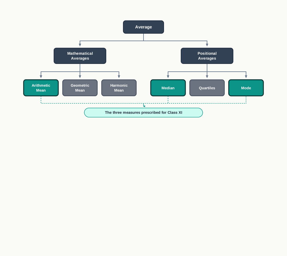
Fig. 18.1 – Types of averages.

The main points of difference between the two categories are set out below.

Compare Table

Each of these averages has its own merits and demerits, and which of them suits a given body of data depends on the data and on the purpose in hand. Of the whole family, the syllabus for Class XI prescribes three — the arithmetic mean, the median and the mode — and it is to these that the rest of the chapter is devoted. The geometric mean, the harmonic mean and the quartiles are named here only so that the classification is complete.

18.2 Arithmetic Mean

18.2.1 Meaning of the Arithmetic Mean

Of all the averages the arithmetic mean is the one in common use, so much so that to most people ‘average’ means nothing else. It is obtained by adding up the values of all the items of a series and dividing the total by the number of items.

The reasoning behind it is a simple one. If the total quantity in a series were shared out equally among all the items, each item would receive the mean — which is why the mean of a set of wages is spoken of as the average wage rate, and the mean of a set of incomes as the average income.

Definition

Arithmetic Mean The arithmetic mean is the number obtained by dividing the sum of the values of all the items of a series by the number of items. In the words of Secrist, it is the amount secured by dividing the sum of the values of the items in a series by their number.

The arithmetic mean of a set of \(N\) values is written as follows.

\[\bar{X} = \dfrac{X_1 + X_2 + X_3 + \ldots + X_n}{N} = \dfrac{\Sigma X}{N}\]

Here \(\bar{X}\), read ‘X bar’, is the arithmetic mean; \(X_1, X_2, X_3 \ldots X_n\) are the \(N\) values taken by the variable \(X\), such as marks or wages or incomes; \(N\) is the number of observations; and \(\Sigma\), the Greek capital letter sigma, stands for ‘the sum of’, so that \(\Sigma X\) is the sum of all the individual values in the series. The mean is expressed in the same unit as the variable itself — rupees, kilograms, marks, years.

The arithmetic mean is of two kinds. In the simple arithmetic mean every item of the series is given equal importance, all items being treated as equally important. In the weighted arithmetic mean the items are given different importance, according to how significant each is. Sections 18.2.2 to 18.2.5 deal with the simple mean; the weighted mean is taken up in Section 18.2.6.

How the simple mean is computed depends on the form the data take, and three forms have to be distinguished — the individual series, the discrete series and the continuous series.

18.2.2 Arithmetic Mean of an Individual Series

An individual series is one in which the values are listed singly and no frequencies are given. Here the mean may be found by either of two methods.

The Direct Method

The direct method applies the basic formula \(\bar{X} = \Sigma X / N\) and takes three steps. Add up the values of all the items to obtain \(\Sigma X\); count the observations to obtain \(N\); divide the first total by the second.

The Short-Cut Method

When the items are many, or their values large, adding them all is laborious. The short-cut method reduces the arithmetic by measuring each item not from zero but from a convenient value close to the centre of the series, called the assumed mean.

\[\bar{X} = A + \dfrac{\Sigma d}{N}\]

Here \(A\) is the assumed mean, \(d\) is the deviation of an item from it, so that \(d = X - A\); \(\Sigma d\) is the sum of these deviations and \(N\) the number of observations. Items larger than \(A\) give positive deviations and items smaller than \(A\) give negative ones, so \(\Sigma d\) may be positive or negative. The quotient \(\Sigma d / N\) is the correction that carries the assumed mean to the true mean.

Any value may be taken as \(A\); a whole number near the middle of the series keeps the working light. If \(A\) happens to equal the actual mean, \(\Sigma d\) works out to zero.

The working is set out in Table 18.1.

Table

Table 18.1 — Working For The Mean Daily Wage By The Short-Cut Method | Worker | Daily wage (₹) X | Deviation from assumed mean (d = X − 500) | |—|—|—| | 1 | 420 | −80 | | 2 | 450 | −50 | | 3 | 480 | −20 | | 4 | 500 | 0 | | 5 | 520 | +20 | | 6 | 560 | +60 | | 7 | 600 | +100 | | 8 | 630 | +130 | | N = 8 | ΣX = 4,160 | Σd = +160 |

Example 18.1

SE 18.1 — Mean Daily Wage By The Direct And Short-Cut Methods

Eight workers at a printing press earn daily wages of ₹420, ₹450, ₹480, ₹500, ₹520, ₹560, ₹600 and ₹630. Calculate the arithmetic mean of the wages by the direct method, and verify the answer by the short-cut method taking ₹500 as the assumed mean; the working is set out in Table 18.1.

By the direct method, from Table 18.1, \(\Sigma X = 4{,}160\) and \(N = 8\)

\(\bar{X} = \dfrac{\Sigma X}{N} = \dfrac{4{,}160}{8} = ₹520\)

By the short-cut method, from Table 18.1, \(A = ₹500\), \(\Sigma d = 160\) and \(N = 8\)

\(\bar{X} = A + \dfrac{\Sigma d}{N} = 500 + \dfrac{160}{8} = 500 + 20 = ₹520\)

The mean daily wage is ₹520, and both methods give the same answer.

18.2.3 Arithmetic Mean of a Discrete Series

In a discrete series each value of the variable is written once and the number of times it occurs is recorded against it as its frequency. An item occurring five times must count five times over in the total, and the formula is adjusted accordingly.

\[\bar{X} = \dfrac{f_1X_1 + f_2X_2 + \ldots + f_nX_n}{f_1 + f_2 + \ldots + f_n} = \dfrac{\Sigma fX}{\Sigma f}\]

Here \(X_1, X_2 \ldots X_n\) are the different values of the variable and \(f_1, f_2 \ldots f_n\) their respective frequencies; \(\Sigma fX\) is the sum of the products of each value and its frequency, and \(\Sigma f\) is the total number of observations. Each value is multiplied by its frequency, the products are added, and the total is divided by the total frequency.

The short-cut method may be used here as well. Deviations are taken from an assumed mean and each is multiplied by the frequency of its own value.

\[\bar{X} = A + \dfrac{\Sigma fd}{\Sigma f}\]

In this formula \(d = X - A\) as before, \(\Sigma fd\) is the sum of the products of the deviations and their frequencies, and \(\Sigma f\) is the total frequency. Where \(\Sigma fd\) is negative, the correction is subtracted from the assumed mean.

The frequencies and the products needed for the direct method are set out in Table 18.2.

Table

Table 18.2 — Working For The Mean Number Of Bicycles Sold Per Day | Bicycles sold per day (X) | Number of days (f) | Product of value and frequency (fX) | |—|—|—| | 2 | 4 | 8 | | 3 | 7 | 21 | | 4 | 10 | 40 | | 5 | 9 | 45 | | 6 | 6 | 36 | | 7 | 4 | 28 | | Total | Σf = 40 | ΣfX = 178 |

Example 18.2

SE 18.2 — Mean Of A Discrete Series By The Direct Method

A cycle dealer records the number of bicycles sold on each of 40 working days. Sales of 2 bicycles occurred on 4 days, 3 on 7 days, 4 on 10 days, 5 on 9 days, 6 on 6 days and 7 on 4 days. Calculate the average number of bicycles sold per day; the working is set out in Table 18.2.

From Table 18.2, \(\Sigma fX = 178\) and \(\Sigma f = 40\)

\(\bar{X} = \dfrac{\Sigma fX}{\Sigma f} = \dfrac{178}{40} = 4.45\) bicycles

The dealer sells 4.45 bicycles a day on average, though no single day’s sale can take that value.

18.2.4 Arithmetic Mean of a Continuous Series

In a continuous series the data are grouped into class intervals such as 10–20 or 20–30, and only the frequency of each class is known, not the individual values within it. The difficulty is met by assuming that the items of a class are spread evenly over it, so that the mid-value of the class may stand for every item in it.

The mid-value is found by adding the lower and upper limits of a class and dividing by two; for the class 20–30 it is \((20 + 30)/2 = 25\). Once each class has been replaced by its mid-value, the series is treated exactly as a discrete series would be.

\[\bar{X} = \dfrac{\Sigma fm}{\Sigma f}\]

Here \(m\) is the mid-value of a class, \(f\) its frequency and \(\Sigma f\) the total frequency; \(\Sigma fm\) is the sum of the products of the mid-values and their frequencies. This is the direct method. The short-cut method takes deviations of the mid-values from an assumed mean, \(d = m - A\), and applies \(\bar{X} = A + \Sigma fd / \Sigma f\).

The Step Deviation Method

Where all the classes are of equal width, the short-cut method can be shortened further. Every deviation \(d\) is then a multiple of the class width, so dividing each by the width leaves a small whole number called the step deviation, written \(d'\).

\[\bar{X} = A + \dfrac{\Sigma fd'}{\Sigma f} \times C\]

Here \(A\) is the assumed mean, \(d' = d / C\) is the step deviation, \(C\) is the size of the class interval and \(\Sigma fd'\) the sum of the products of the step deviations and their frequencies. Since dividing by \(C\) shrinks every deviation, the correction must be multiplied by \(C\) to restore the scale. The method is also called the coding method, and it is the one to use whenever the class intervals are equal.

The working by this method is set out in Table 18.3.

Table

Table 18.3 — Working For The Mean Monthly Expenditure On Food By The Step Deviation Method | Monthly expenditure (₹) | Households (f) | Mid-value (m) | Step deviation (d′ = (m − 4,500) ÷ 1,000) | Product (fd′) | |—|—|—|—|—| | 2,000–3,000 | 5 | 2,500 | −2 | −10 | | 3,000–4,000 | 10 | 3,500 | −1 | −10 | | 4,000–5,000 | 16 | 4,500 | 0 | 0 | | 5,000–6,000 | 14 | 5,500 | +1 | +14 | | 6,000–7,000 | 9 | 6,500 | +2 | +18 | | 7,000–8,000 | 6 | 7,500 | +3 | +18 | | Total | Σf = 60 | | | Σfd′ = +30 |

Example 18.3

SE 18.3 — Mean Of A Continuous Series By The Step Deviation Method

The monthly expenditure on food of 60 households in a locality is distributed as follows: ₹2,000–3,000, 5 households; ₹3,000–4,000, 10; ₹4,000–5,000, 16; ₹5,000–6,000, 14; ₹6,000–7,000, 9; ₹7,000–8,000, 6. Calculate the mean monthly expenditure on food, taking ₹4,500 as the assumed mean; the working is set out in Table 18.3.

From Table 18.3, \(A = ₹4{,}500\), \(\Sigma fd' = 30\), \(\Sigma f = 60\) and \(C = ₹1{,}000\)

\(\bar{X} = A + \dfrac{\Sigma fd'}{\Sigma f} \times C\)

\(\bar{X} = 4{,}500 + \dfrac{30}{60} \times 1{,}000\)

\(\bar{X} = 4{,}500 + 500 = ₹5{,}000\)

The mean monthly expenditure on food is ₹5,000 per household.

Exam Pointer

The step deviation working is not finished until the correction has been multiplied by C. Dropping that multiplication is the commonest error in these numericals, and it leaves the answer far too close to the assumed mean.

18.2.5 Special Problems in Calculating the Arithmetic Mean

Data do not always arrive in a form ready for the formulas above. Four situations call for an adjustment before the mean can be computed.

Cumulative frequency distributions — where the data are given as a ‘less than’ or ‘more than’ series, the simple frequency of each class must be recovered first. In a ‘less than’ series the frequency of a class is found by deducting the cumulative frequency of the preceding class from that of the class itself; in a ‘more than’ series each cumulative frequency is reduced by the one below it. The mean is then computed in the usual way.
Open-end classes — where the lower limit of the first class or the upper limit of the last is not stated, the missing limit has to be supplied before a mid-value can be found. It is assumed on the pattern of the other classes: if the stated classes are all of width 10 and the first is ‘below 10’, its lower limit is taken as 0, and if the last is ‘above 40’, its upper limit is taken as 50.
Correcting a wrong value — where an item has been copied wrongly and the mean already computed from it, the incorrect total is recovered as \(\Sigma X = \bar{X} \times N\), the wrong value is deducted from it and the right one added.

\[\text{Correct } \bar{X} = \dfrac{\text{Incorrect } \Sigma X - \text{Incorrect value} + \text{Correct value}}{N}\]

A missing item or frequency — where the mean is known but one value or one frequency is not, the unknown is written as \(X\) or \(f\), the direct-method formula is applied as an equation, and the equation is solved for the unknown.

Watch Out

Assuming a limit for an open-end class changes the mid-value of that class and so changes the mean. Always state the assumption you have made.

18.2.6 Weighted Arithmetic Mean

The simple arithmetic mean treats every item as equally important. In many series they are not. A household spends far more on food than on entertainment, so an average of the price changes it faces cannot give the two items equal standing; a student’s subjects may carry different credit; a factory may employ far more workers on one wage rate than on another.

In such cases the relative importance of each item must enter the calculation. The figure attached to an item to express that importance is its weight, and the average so obtained is the weighted arithmetic mean.

\[\bar{X}_w = \dfrac{\Sigma WX}{\Sigma W}\]

Here \(\bar{X}_w\) is the weighted arithmetic mean, \(X\) the different values of the variable, \(W\) the weight attached to each value, \(\Sigma WX\) the sum of the products of the values and their weights, and \(\Sigma W\) the sum of the weights. The unit is that of the variable. The working is the same as for a discrete series, with the weight \(W\) standing where the frequency \(f\) stood.

The working is set out in Table 18.4.

Table

Table 18.4 — Working For The Weighted Mean Price Of Rice | Grade of rice | Price per kg (₹) X | Quantity sold in kg (W) | Product (WX) | |—|—|—|—| | Ordinary | 40 | 120 | 4,800 | | Medium | 55 | 60 | 3,300 | | Fine | 70 | 20 | 1,400 | | Total | | ΣW = 200 | ΣWX = 9,500 |

Example 18.4

SE 18.4 — Weighted Mean Price Of Rice

A fair price shop sells three grades of rice in a month — ordinary at ₹40 per kg, medium at ₹55 per kg and fine at ₹70 per kg. The quantities sold are 120 kg, 60 kg and 20 kg respectively. Calculate the weighted mean price of the rice sold, taking the quantities as weights; the working is set out in Table 18.4.

From Table 18.4, \(\Sigma WX = 9{,}500\) and \(\Sigma W = 200\)

\(\bar{X}_w = \dfrac{\Sigma WX}{\Sigma W} = \dfrac{9{,}500}{200} = ₹47.50\) per kg

The weighted mean price is ₹47.50 per kg, well below the simple mean of ₹55, because most of the rice sold was of the cheapest grade.

Economy Example

Average Size Of A Landholding The Agriculture Census divides the total operated area in India by the number of operational holdings to obtain the average size of a holding. Successive censuses have shown that average falling, as holdings are divided among heirs from one generation to the next. The single figure is what makes the trend across decades visible at all.

18.2.7 Properties of the Arithmetic Mean

The arithmetic mean has mathematical properties that no positional average shares, and it is these that make it so useful in further statistical work.

The sum of the deviations of the items from the mean is zero — that is, \(\Sigma (X - \bar{X}) = 0\). The positive deviations of the items above the mean exactly cancel the negative deviations of those below it, which is another way of saying that the mean is the point of balance of a series.
The sum of the squares of the deviations from the mean is minimum — the squared deviations taken from the mean total less than those taken from any other value. This property makes the mean the natural base from which to measure dispersion in the next chapter.
The product of the mean and the number of observations equals the sum of all the values — since \(\bar{X} = \Sigma X / N\), it follows that \(N\bar{X} = \Sigma X\). Knowing the average wage in a factory and the number of workers, we can at once compute the total wage bill.
The means of two or more groups can be combined — where the mean of each group and the number of items in it are known, the mean of the groups taken together may be computed without returning to the original data.

\[\bar{X}_{12} = \dfrac{N_1\bar{X}_1 + N_2\bar{X}_2}{N_1 + N_2}\]

Here \(\bar{X}_{12}\) is the combined mean of the two groups, \(\bar{X}_1\) and \(\bar{X}_2\) are their separate means, and \(N_1\) and \(N_2\) the number of items in each. The formula extends to any number of groups, the numerator taking one product for each group and the denominator the total of all the items.

18.2.8 Merits and Demerits of the Arithmetic Mean

The arithmetic mean meets most of the conditions of a good average laid down in Section 18.1.4, and its merits follow from them.

Certainty — the mean is rigidly defined, so its value is definite and leaves no room for differing interpretation.
Based on all observations — every item of the series enters the calculation, which makes the mean the most representative of the three measures.
Simplicity — it is the easiest of the averages to understand and to compute, and it is the one a common reader already has in mind when the word average is used.
Capable of algebraic treatment — the properties set out in Section 18.2.7 allow the mean to be used in further mathematical work, which is why it is so extensively employed in statistical analysis.
Stability — it is affected less than other averages by changes in the sample drawn from a population, and so gives comparatively steady results.

Against these stand real limitations, and they are limitations of exactly the same feature — that the mean uses every value in the series.

Affected by extreme values — one very small or very large item pulls the mean towards itself. A student scoring 80, 85 and 65 marks in three subjects and 10 in a fourth has a mean of 60, which represents none of the four results.
Cannot be computed from incomplete data — since every item is needed, a single missing value makes the mean impossible to calculate directly.
May not figure in the series — the mean of 4, 8, 15 and 21 is 12, and no item in that series has the value 12.
May give absurd results — where the variable can take only whole values, the mean may not. An average of 3.4 children per family is arithmetically correct and descriptively impossible.
May mislead — three workers earning ₹600, ₹700 and ₹800 a day and three earning ₹600, ₹300 and ₹1,200 have the same mean daily wage of ₹700, though the two groups are not alike at all. The mean reports the centre and is silent about the spread.

The mean, then, should be used with judgement rather than by habit. It remains the most widely used measure of central value in practice, and the average income, average expenditure, average cost and average revenue of economics are all arithmetic means.

18.3 Median

18.3.1 Meaning of the Median

The arithmetic mean answers the question ‘what would each item get if the total were shared equally?’ The median answers a different one: ‘which item stands at the centre when the series is arranged in order?’

The median is the value of the variable that divides a series into two equal parts, so that half the observations have values greater than it and half have values smaller. Arrange the weights of five persons in ascending order as 50, 55, 62, 65 and 70 kg, and the median weight is 62 kg — two items lie below it and two above.

Definition

Median The median is that value of the variable which divides the group into two equal parts, one part comprising all values greater than the median value and the other part comprising all values smaller than it. This definition is due to Connor.

The median is a positional average. Its value is settled by the place an item occupies in an ordered series, not by the size of the other items, and unlike the arithmetic mean it does not take their values into account at all. That is why the median is particularly useful where the items cannot be measured exactly. Average intelligence or average health cannot be added and divided, but a group of persons can still be arranged in order and the middle one identified.

The median may be found by two methods — the algebraic method, which computes it from a formula, and the graphic method, which reads it off a curve. Both are taken up below, the algebraic method first.

18.3.2 Median of an Individual Series

Since the median is defined by position, the first step in every case is to put the raw data into an array — that is, to arrange the items in ascending or descending order of magnitude. Either order gives the same median. The number of items \(N\) is then counted, and the position of the median item located.

\[M = \text{size of } \left(\dfrac{N + 1}{2}\right)\text{th item}\]

Here \(M\) is the median and \(N\) the number of observations. The formula gives the position of the median in the array, not its value; the value is then read off from the item standing in that position, and carries the unit of the variable.

Where \(N\) is odd, \((N+1)/2\) is a whole number and the median is simply the value of that item. Where \(N\) is even, \((N+1)/2\) falls halfway between two items, and the median is taken as the average of the two values lying on either side of it. In that case the median does not coincide with any item of the series.

Example 18.5

SE 18.5 — Median Monthly Rent Of Shops

The monthly rents paid by nine shops in a market are ₹4,000, ₹4,500, ₹5,000, ₹5,200, ₹5,800, ₹6,000, ₹6,500, ₹7,000 and ₹9,500. Calculate the median rent. Calculate it again for the ten shops that result when a tenth shop paying ₹12,000 joins the market.

The items are already arranged in ascending order.

For nine shops, \(N = 9\)

\(M = \text{size of } \left(\dfrac{9 + 1}{2}\right)\text{th item} = \text{size of the 5th item}\)

\(M = ₹5{,}800\)

For ten shops, \(N = 10\)

\(M = \text{size of } \left(\dfrac{10 + 1}{2}\right)\text{th item} = \text{size of the 5.5th item}\)

\(M = \dfrac{\text{5th item} + \text{6th item}}{2} = \dfrac{5{,}800 + 6{,}000}{2} = ₹5{,}900\)

The median rent is ₹5,800 for nine shops and ₹5,900 for ten, the addition of a rent of ₹12,000 having moved it by only ₹100.

18.3.3 Median of a Discrete Series

In a discrete series the values are already arranged in order and each carries a frequency, so the middle item has to be traced through the frequencies. This is done by cumulating them — adding each frequency to the total of those before it — to obtain the cumulative frequency of every value.

\[M = \text{value of } \left(\dfrac{N + 1}{2}\right)\text{th item, where } N = \Sigma f\]

Here \(N\) is the total of the frequencies. The position of the median item is found as before; the cumulative frequency column is then read down until the first cumulative frequency equal to or greater than that position is reached, and the value standing against it is the median.

The cumulative frequencies are set out in Table 18.5.

Table

Table 18.5 — Working For The Median Number Of Days Of Work Obtained In A Week | Days of work in a week (X) | Number of labourers (f) | Cumulative frequency (c.f.) | |—|—|—| | 1 | 3 | 3 | | 2 | 7 | 10 | | 3 | 12 | 22 | | 4 | 10 | 32 | | 5 | 8 | 40 | | 6 | 5 | 45 | | Total | Σf = 45 | |

Example 18.6

SE 18.6 — Median Of A Discrete Series

A survey of 45 casual labourers records the number of days of work each obtained in a particular week: 1 day, 3 labourers; 2 days, 7; 3 days, 12; 4 days, 10; 5 days, 8; 6 days, 5. Calculate the median number of days of work; the working is set out in Table 18.5.

From Table 18.5, \(N = \Sigma f = 45\)

\(M = \text{value of } \left(\dfrac{45 + 1}{2}\right)\text{th item} = \text{value of the 23rd item}\)

The 22nd item falls in the cumulative frequency 22 and the 32nd in the cumulative frequency 32, so the 23rd item lies against the value 4.

\(M = 4\) days

The median labourer obtained 4 days of work in the week.

18.3.4 Median of a Continuous Series

In a continuous series the individual values are lost inside the class intervals, so the median cannot simply be picked out. It is located in two stages: the class containing the median is identified first, and its exact value within that class is then estimated.

The class containing the median is called the median class. It is found by cumulating the frequencies and reading down the cumulative frequency column to the first class whose cumulative frequency equals or exceeds \(N/2\). Note the change: for a continuous series the median position is taken as \(N/2\), not \((N+1)/2\), because the items are treated as spread continuously over the classes rather than counted one by one.

Having found the class, the median is estimated within it on the assumption that the items are spread evenly across the interval.

\[M = L_1 + \left(\dfrac{\dfrac{N}{2} - c.f.}{f_{\text{median}}}\right) \times C\]

Here \(L_1\) is the lower limit of the median class; \(N\) is the total frequency \(\Sigma f\); \(c.f.\) is the cumulative frequency of the class immediately preceding the median class; \(f_{\text{median}}\) is the frequency of the median class itself; and \(C\) is the width of the median class. The bracketed fraction is the proportion of the median class that must be crossed to reach the middle item, and multiplying it by \(C\) converts that proportion into units of the variable. The answer carries the unit of the variable.

The cumulative frequencies are set out in Table 18.6.

Table

Table 18.6 — Working For The Median Weight Of Students | Weight (kg) | Number of students (f) | Cumulative frequency (c.f.) | |—|—|—| | 30–35 | 4 | 4 | | 35–40 | 9 | 13 | | 40–45 | 14 | 27 | | 45–50 | 18 | 45 | | 50–55 | 10 | 55 | | 55–60 | 5 | 60 | | Total | Σf = 60 | |

Example 18.7

SE 18.7 — Median Of A Continuous Series

The weights of 60 students of a class are distributed as follows: 30–35 kg, 4 students; 35–40 kg, 9; 40–45 kg, 14; 45–50 kg, 18; 50–55 kg, 10; 55–60 kg, 5. Calculate the median weight; the working is set out in Table 18.6.

From Table 18.6, \(N = \Sigma f = 60\)

\(\dfrac{N}{2} = \dfrac{60}{2} = 30\)th item

The cumulative frequency 27 falls short of 30 and the next cumulative frequency 45 exceeds it, so the median class is 45–50.

\(L_1 = 45\), \(c.f. = 27\), \(f_{\text{median}} = 18\), \(C = 5\)

\(M = 45 + \left(\dfrac{30 - 27}{18}\right) \times 5\)

\(M = 45 + \dfrac{3}{18} \times 5 = 45 + 0.83\)

\(M = 45.83\) kg

The median weight of the students is 45.83 kg.

Watch Out

The median class is the class in which the cumulative frequency first reaches N ÷ 2. It is not the class with the highest frequency — that one belongs to the mode.

18.3.5 Special Problems in Calculating the Median

Three situations require attention before the formula of Section 18.3.4 can be applied.

Cumulative frequency distributions — where the data are given as a ‘less than’ or ‘more than’ series, the simple frequency of each class must be recovered first, exactly as for the mean. Only then can the frequency of the median class be read.
Mid-values given instead of classes — where the series lists mid-values alone, the class intervals must be reconstructed. The width is the difference between two consecutive mid-values, and half of it is subtracted from and added to each mid-value to obtain the limits of its class.
Unequal class intervals — no adjustment is needed. The formula takes the width \(C\) of the median class alone, so classes of differing width cause no difficulty here, though they do for the mode.

The simple frequencies recovered from a ‘less than’ series are set out in Table 18.7.

Table

Table 18.7 — Working For The Median Annual Income Of Farmers | Annual income (₹ thousand) | Number of farmers (f) | Cumulative frequency (c.f.) | |—|—|—| | 0–20 | 8 | 8 | | 20–40 | 14 | 22 | | 40–60 | 23 | 45 | | 60–80 | 23 | 68 | | 80–100 | 12 | 80 | | Total | Σf = 80 | |

Example 18.8

SE 18.8 — Median From A ‘Less Than’ Cumulative Distribution

The annual incomes of 80 farmers in a block are reported as follows: less than ₹20 thousand, 8 farmers; less than ₹40 thousand, 22; less than ₹60 thousand, 45; less than ₹80 thousand, 68; less than ₹100 thousand, 80. Calculate the median annual income; the working is set out in Table 18.7.

Each simple frequency is obtained by deducting the cumulative frequency of the preceding class, as shown in Table 18.7.

\(N = \Sigma f = 80\)

\(\dfrac{N}{2} = \dfrac{80}{2} = 40\)th item

The cumulative frequency 22 falls short of 40 and the next cumulative frequency 45 exceeds it, so the median class is 40–60.

\(L_1 = 40\), \(c.f. = 22\), \(f_{\text{median}} = 23\), \(C = 20\)

\(M = 40 + \left(\dfrac{40 - 22}{23}\right) \times 20\)

\(M = 40 + \dfrac{18}{23} \times 20 = 40 + 15.65\)

\(M = ₹55.65\) thousand

The median annual income is ₹55,650, so half the farmers in the block earn less than this.

Exam Pointer

Use (N + 1) ÷ 2 to locate the median item in an individual or discrete series, and N ÷ 2 in a continuous series. Marks are regularly lost by carrying the first rule into a grouped distribution.

18.3.6 Graphic Determination of the Median

The median can also be read off a graph, which is one of its advantages over the arithmetic mean. The curve used is the cumulative frequency curve, or ogive, drawn with the values of the variable on the X-axis and the cumulative frequencies on the Y-axis.

The steps are these. Convert the distribution into a ‘less than’ or a ‘more than’ cumulative frequency series and plot the ogive. Locate \(N/2\) on the Y-axis and draw a line from it parallel to the X-axis until it cuts the ogive. From that point of intersection drop a perpendicular to the X-axis; the value at which it meets the axis is the median. The ‘less than’ ogive for the data of Table 18.6 is drawn in Fig. 18.2.

Fig. 18.2

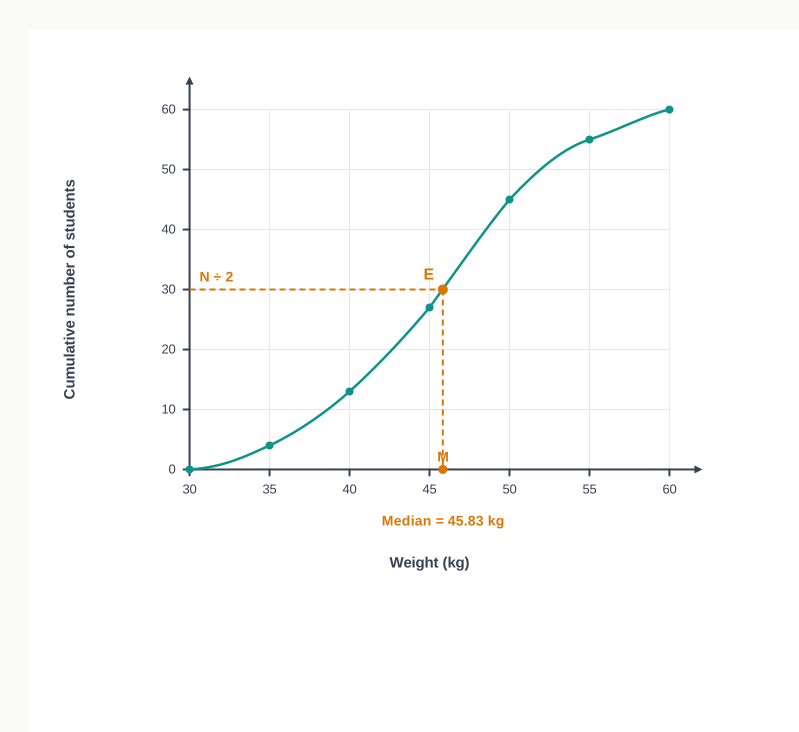
Fig. 18.2 – Locating the median on a ‘less than’ ogive.

Alternatively both ogives may be drawn together. The ‘less than’ ogive rises from left to right and the ‘more than’ ogive falls, and the two must cross at the value below which and above which equal numbers of items lie — which is the median itself. A perpendicular dropped from the point of intersection to the X-axis gives the median directly, without any need to locate \(N/2\) on the Y-axis. Fig. 18.3 shows the same data treated in this way.

Fig. 18.3

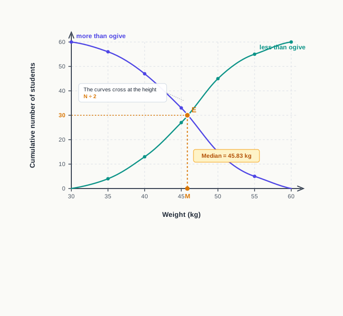
Fig. 18.3 – Median from simultaneous ogives.

18.3.7 Merits and Demerits of the Median

The median has merits of its own, several of which follow from its being a positional average.

Certainty — the median is rigidly defined, so its value is definite and free from ambiguity.
Simplicity — it is easy to understand and easy to compute, and in a short series it can be found merely by inspecting the arrayed data.
Unaffected by extreme values — since only position counts, an unusually large or small item cannot pull the median away from the centre of the series.
Possible even with incomplete data — the median can be found although some values are unknown, provided the number of items and the middle item are known.
Open to graphic treatment — it can be located from an ogive, as Section 18.3.6 shows, which no other average of this chapter can match for ease.
Suited to qualitative data — where a characteristic cannot be measured but the items can be ranked, as with intelligence or ability, the median is the only average that can be used at all.

Its limitations are the counterpart of the same feature.

Not based on all observations — the median ignores the values of every item except those at the centre, and so does not use all the information the data contain.
May lack representative character — in a small series, or one in which the items vary widely, the middle value may not describe the series well.
Affected by sampling fluctuations — the value of the median shifts more than that of the mean when a different sample is drawn from the same population.
Not capable of algebraic treatment — the medians of two groups cannot be combined into the median of the two taken together, as the means can.

Economy Example

Why A Typical Income Is Reported As A Median In a village where one landowner earns many times what everyone else does, the mean income can exceed what almost every household actually earns. The median household is unmoved by that single large income, so it describes the typical villager far more faithfully. This is why studies of income and consumption so often report the median alongside the mean.

18.4 Mode

18.4.1 Meaning of the Mode

The mean asks what each item would get on an equal division and the median asks which item stands at the centre. The mode asks a third question, and often the most practical one: which value occurs most often?

The mode of a set of observations is the value that occurs the greatest number of times, that is, with the greatest frequency in the series. Put more strictly, it is the value around which the items are most heavily concentrated, and so the most typical value the series contains. It is written as \(Z\).

Definition

Mode The mode of a distribution is the value around which the items tend to be most heavily concentrated. It may be regarded as the most typical of a series of values. In a frequency distribution the mode is the value that occurs with the greatest frequency.

There are situations in which the mode describes data better than either of the other averages can. A manufacturer of readymade garments needs to know which size is bought most often, not the arithmetic average of all sizes bought. If the modal shoe size is 7, the largest number of buyers wear that size, and production is planned accordingly. If the modal wage rate in a factory is ₹300 a day, more workers receive that rate than any other.

A distribution having only one mode is called a unimodal distribution. Where two values share the maximum frequency the distribution has two modes and is called a bimodal distribution; where more than two do, it is multimodal. In such cases the mode is not uniquely determined, and this is a real weakness of the measure.

Economy Example

Sizing A Garment Production Run A firm producing readymade shirts cannot manufacture equal numbers of every size. It studies the sizes actually sold across its stores and produces most heavily in the modal size, tapering output on either side of it. The mean size would be useless here, since it might fall between two sizes that no customer asks for.

18.4.2 Mode of an Individual Series

In a series of individual observations the mode may be found in either of two ways.

By inspection, the data are first arranged in the form of an array, and the number of times each value repeats itself is counted. The value occurring most frequently is the mode. This works well when the items are few.

By converting to a frequency series, the individual items are tabulated against the number of times each occurs, and the value standing against the highest frequency is taken as the mode. Where the items are many, the frequencies are counted with a tally or score sheet.

Example 18.9

SE 18.9 — Mode Of An Individual Series

The collar sizes of the fifteen shirts sold at a shop on one day were 38, 40, 42, 40, 44, 40, 42, 38, 40, 42, 44, 40, 42, 40 and 38. Determine the modal collar size.

Arranging the items as an array: 38, 38, 38, 40, 40, 40, 40, 40, 40, 42, 42, 42, 42, 44, 44

Size 38 occurs 3 times

Size 40 occurs 6 times

Size 42 occurs 4 times

Size 44 occurs 2 times

\(Z = 40\)

The modal collar size is 40, this being the size sold to the largest number of buyers.

18.4.3 Mode of a Discrete Series

In a discrete series the frequencies are already given, and the mode may often be located simply by inspection — by identifying the value that carries the highest frequency. The frequency series obtained in SE 18.9 is a case of this kind: size 40 carries the frequency 6, no other size comes near it, and the mode is read off at once.

Inspection is dependable only where the series is regular and homogeneous. It becomes unsafe in two situations: where the items are heavily concentrated at more than one value, and where the difference between the highest frequency and the next highest is very small. A single frequency then decides the answer, and a small irregularity in the data can move the mode from one value to another.

In such cases the mode is determined by the grouping method, which examines not the frequency of each value alone but the weight of frequency in the neighbourhood of each value.

Watch Out

The highest frequency in a discrete series is not always at the mode. Where two frequencies are close, use the grouping method before answering.

18.4.4 The Grouping Table and the Analysis Table

The grouping method rests on a simple idea. A value is modal not merely because its own frequency is large but because the values on either side of it also carry large frequencies, so that the items are concentrated about it. The method therefore adds frequencies in twos and in threes, in every way in which consecutive values can be combined, and sees which value keeps appearing in the largest totals.

It uses two tables. The grouping table carries six columns: column 1 holds the original frequencies; columns 2 and 3 holds them grouped in twos, beginning with the first and the second item respectively; and columns 4, 5 and 6 holds them grouped in threes, beginning with the first, the second and the third item respectively. Each grouped total is entered against the first item of the group it covers, and the largest total in each column is identified.

The analysis table then records, for each column of the grouping table, the values that make up its largest total. The value receiving the greatest number of entries is the mode.

The grouping is set out in Table 18.8 and the analysis in Table 18.9.

Table

Table 18.8 — Grouping Table For The Number Of Goats Owned By Farmers | Number of goats (X) | Frequencies (1) | Grouped in twos from the 1st item (2) | Grouped in twos from the 2nd item (3) | Grouped in threes from the 1st item (4) | Grouped in threes from the 2nd item (5) | Grouped in threes from the 3rd item (6) | |—|—|—|—|—|—|—| | 2 | 6 | 15 | — | 29 | — | — | | 3 | 9 | — | 23 | — | 41 | — | | 4 | 14 | 32 | — | — | — | 49 | | 5 | 18 | — | 35 | 55 | — | — | | 6 | 17 | 37 | — | — | 45 | — | | 7 | 20 | — | 28 | — | — | 36 | | 8 | 8 | 16 | — | 16 | — | — | | 9 | 8 | — | — | — | — | — |

Table

Table 18.9 — Analysis Table For The Number Of Goats Owned By Farmers | Column of the grouping table | 4 | 5 | 6 | 7 | 8 | |—|—|—|—|—|—| | 1 | — | — | — | ✓ | — | | 2 | — | — | ✓ | ✓ | — | | 3 | — | ✓ | ✓ | — | — | | 4 | — | ✓ | ✓ | ✓ | — | | 5 | — | — | ✓ | ✓ | ✓ | | 6 | ✓ | ✓ | ✓ | — | — | | Total entries | 1 | 3 | 5 | 4 | 1 |

Example 18.10

SE 18.10 — Mode Of A Discrete Series By The Grouping Method

A survey of 100 farmers records the number of goats owned by each: 2 goats, 6 farmers; 3 goats, 9; 4 goats, 14; 5 goats, 18; 6 goats, 17; 7 goats, 20; 8 goats, 8; 9 goats, 8. Determine the modal number of goats owned; the grouping is set out in Table 18.8 and the analysis in Table 18.9.

By inspection the highest single frequency is 20, which stands against 7 goats.

The largest total in each column of Table 18.8 is 20 in column 1, against 7 goats; 37 in column 2, against 6 and 7; 35 in column 3, against 5 and 6; 55 in column 4, against 5, 6 and 7; 45 in column 5, against 6, 7 and 8; and 49 in column 6, against 4, 5 and 6.

From the totals of Table 18.9, the value 6 carries 5 entries, more than any other value.

\(Z = 6\) goats

The modal holding is 6 goats, not the 7 that inspection alone suggested, because the frequencies on both sides of 6 are heavier than those around 7.

18.4.5 Mode of a Continuous Series

In a continuous series the individual values are lost inside the class intervals, so the mode is found in two stages, much as the median was. The class in which the mode lies, called the modal class, is identified first, by inspection or by the grouping method; its exact value within that class is then estimated.

\[Z = L_1 + \dfrac{f_1 - f_0}{2f_1 - f_0 - f_2} \times C\]

Here \(Z\) is the mode; \(L_1\) is the lower limit of the modal class; \(f_1\) is the frequency of the modal class; \(f_0\) is the frequency of the class preceding it; \(f_2\) is the frequency of the class succeeding it; and \(C\) is the width of the modal class. The fraction compares the excess of the modal frequency over the preceding class with its excess over both neighbours together, so the mode is pulled towards whichever neighbour is the heavier. The answer carries the unit of the variable.

Example 18.11

SE 18.11 — Mode Of A Continuous Series

The daily sales of a kirana shop over 80 working days are distributed as follows: ₹2,000–4,000, 8 days; ₹4,000–6,000, 14; ₹6,000–8,000, 26; ₹8,000–10,000, 18; ₹10,000–12,000, 9; ₹12,000–14,000, 5. Calculate the modal value of daily sales.

The highest frequency is 26, so the modal class is ₹6,000–8,000.

\(L_1 = 6{,}000\), \(f_1 = 26\), \(f_0 = 14\), \(f_2 = 18\), \(C = 2{,}000\)

\(Z = 6{,}000 + \dfrac{26 - 14}{(2 \times 26) - 14 - 18} \times 2{,}000\)

\(Z = 6{,}000 + \dfrac{12}{52 - 32} \times 2{,}000\)

\(Z = 6{,}000 + \dfrac{12}{20} \times 2{,}000 = 6{,}000 + 1{,}200\)

\(Z = ₹7{,}200\)

Daily sales of about ₹7,200 occur more often than sales of any other amount.

Two adjustments are sometimes needed before the formula can be used. Where only the mid-values of the classes are given, the class limits must be reconstructed from them, half the common width being subtracted from and added to each mid-value. Where the data are given as a cumulative series, the simple frequencies must be recovered first.

A third adjustment is more important, because the formula assumes classes of equal width. Where the widths are unequal, the frequency of a wide class is not comparable with that of a narrow one, and the modal class cannot be identified honestly until the classes have been made equal and the frequencies adjusted in proportion. A class of width 20 carrying a frequency of 18 becomes two classes of width 10 carrying 9 each.

The adjusted distribution is set out in Table 18.10.

Table

Table 18.10 — Working For The Mode Of A Series With Unequal Class Intervals | Monthly savings (₹ hundred) as given | Households as given | Adjusted class of equal width | Adjusted frequency | |—|—|—|—| | 0–10 | 4 | 0–10 | 4 | | 10–30 | 18 | 10–20 | 9 | | — | — | 20–30 | 9 | | 30–40 | 20 | 30–40 | 20 | | 40–50 | 12 | 40–50 | 12 | | 50–60 | 6 | 50–60 | 6 | | Total | 60 | | 60 |

Example 18.12

SE 18.12 — Mode Of A Series With Unequal Class Intervals

The monthly savings of 60 households, in hundreds of rupees, are distributed as follows: 0–10, 4 households; 10–30, 18; 30–40, 20; 40–50, 12; 50–60, 6. Calculate the modal monthly saving; the adjustment of the classes is set out in Table 18.10.

The class 10–30 is of double width, so it is split into 10–20 and 20–30 with the frequency of 18 divided equally between them, as shown in Table 18.10.

The highest frequency in the adjusted series is 20, so the modal class is 30–40.

\(L_1 = 30\), \(f_1 = 20\), \(f_0 = 9\), \(f_2 = 12\), \(C = 10\)

\(Z = 30 + \dfrac{20 - 9}{(2 \times 20) - 9 - 12} \times 10\)

\(Z = 30 + \dfrac{11}{40 - 21} \times 10 = 30 + \dfrac{11}{19} \times 10\)

\(Z = 30 + 5.79 = 35.79\)

The modal monthly saving is ₹3,579.

Exam Pointer

Write the denominator of the mode formula as 2f₁ − f₀ − f₂, with both frequencies subtracted. Adding f₂ instead of subtracting it is the standard slip, and it gives an answer that no longer lies inside the modal class.

18.4.6 Graphic Determination of the Mode

The mode of a continuous series can also be located from a histogram, and the construction shows clearly what the formula is doing. The tallest rectangle marks the modal class; the mode is then placed within it, nearer to whichever neighbouring rectangle is the taller.

The steps are these. Draw the histogram of the distribution and identify the rectangle of greatest height, which is the modal class. From the upper right corner of that rectangle draw a straight line to the upper right corner of the preceding rectangle, and from its upper left corner a line to the upper left corner of the succeeding rectangle. From the point at which these two lines cross, drop a perpendicular to the X-axis; the value at which it meets the axis is the mode. The construction for the data of SE 18.11 is shown in Fig. 18.4.

Fig. 18.4

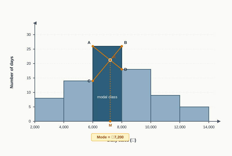
Fig. 18.4 – Locating the mode on a histogram.

The graphic method works only where a single class carries the highest frequency. Where two or more classes share it, the tallest rectangle cannot be identified and the mode cannot be located this way.

18.4.7 Merits and Demerits of the Mode

The merits of the mode are those of a measure that reports the most usual case.

Simplicity — the mode is easy to understand and easy to compute, and in a short series it can be found by mere inspection, though the grouping method is admittedly cumbersome.
Unaffected by extreme values — an extremely large or small item does not disturb the mode, since it contributes nothing to the frequency at the point of concentration.
Open to graphic determination — the mode can be located from a histogram, as Section 18.4.6 shows.
No need of complete data — it is enough to know the values around which the items concentrate; the whole series need not be known.
Representative in practice — because it is the value occurring most often, the mode is the average people actually use in daily life, as with the usual size of readymade garments.

Its demerits are serious enough to keep it from general use.

Indeterminate — the mode cannot be determined at all in a bimodal or multimodal distribution, since no single value carries the maximum frequency.
Not a true representative — it takes no account of the values of the other items, so it does not describe the series as a whole.
Uncertainty — it is not rigidly defined, and different methods of computing it may give different answers for the same data, as SE 18.10 shows.
Not capable of algebraic treatment — the modes of two series cannot be combined into the mode of the two taken together.

18.5 Relationship Between Mean, Median and Mode

18.5.1 The Symmetrical Distribution

Three averages have now been computed from the same kind of data by three different routes — the mean from the values of all the items, the median from the position of the middle item, the mode from the point of heaviest concentration. It is natural to ask how the three answers stand in relation to one another.

The answer depends on the shape of the distribution. Where the items are spread evenly on both sides of the centre, so that the frequency curve is bell shaped and one half is the mirror image of the other, the distribution is said to be symmetrical. In such a distribution the point of balance, the middle position and the point of greatest concentration are one and the same, and the three averages coincide.

\[\bar{X} = M = Z\]

Fig. 18.5 shows this case.

Fig. 18.5

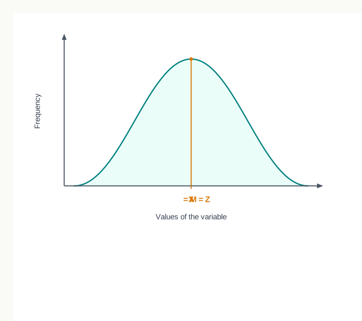
Fig. 18.5 – Symmetrical distribution.

18.5.2 Positively Skewed and Negatively Skewed Distributions

Distributions met in practice are rarely symmetrical. Most are skewed — stretched out further on one side of the peak than on the other — and the three averages then part company in a regular and predictable way.

A distribution is positively skewed when the longer tail lies to the right, that is, when a small number of unusually large items pull the curve out in that direction. The mode stays at the peak, where the items are thickest. The median, dividing the items by count, is displaced somewhat towards the tail. The mean, which uses the actual size of every item, is dragged furthest of all, because the few large values enter the total at their full weight.

\[Z < M < \bar{X}\]

A distribution is negatively skewed when the longer tail lies to the left, a small number of unusually small items stretching the curve in that direction. The same reasoning applies in reverse, and the order of the three averages is exactly inverted.

\[\bar{X} < M < Z\]

In both cases the median lies between the other two, and closer to the mean than to the mode. Figures 18.6 and 18.7 show the two cases.

Fig. 18.6

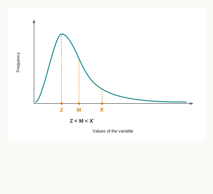
Fig. 18.6 – Positively skewed distribution.

Fig. 18.7

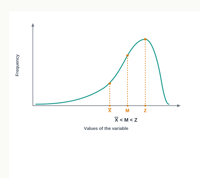
Fig. 18.7 – Negatively skewed distribution.

The main points of difference between the two kinds of skewness are set out below.

Compare Table

Economy Example

Firm Size In Indian Industry Most enterprises in India are small, while a handful employ workers and turn over revenue on an altogether different scale. The distribution of firm size is therefore strongly positively skewed, and its mean overstates the size of the firm a visitor to any industrial cluster would actually find. The modal firm remains a very small one.

18.5.3 The Empirical Relationship

For a moderately skewed distribution the three averages stand in a definite numerical relation, which Karl Pearson expressed as follows.

\[Z = 3M - 2\bar{X}\]

Here \(Z\) is the mode, \(M\) the median and \(\bar{X}\) the arithmetic mean, all three measured in the unit of the variable. The relation says that the distance from the mean to the mode is about three times the distance from the mean to the median — that is, the mode lies about twice as far from the mean as the median does, on the same side of it.

The relation is of practical use because it supplies whichever of the three is missing. It may be transposed to give the median or the mean.

\[M = \dfrac{Z + 2\bar{X}}{3} \qquad \bar{X} = \dfrac{3M - Z}{2}\]

Its main service is in supplying the mode. Where a distribution is bimodal, or has open-end classes, or is otherwise so irregular that the formula of Section 18.4.5 cannot be applied, the mode may still be estimated from the mean and the median, both of which are always computable.

Example 18.13

SE 18.13 — Estimating The Mode From The Mean And The Median

In a moderately asymmetrical distribution of daily earnings, the arithmetic mean is ₹560 and the median is ₹575. Estimate the value of the mode.

\(Z = 3M - 2\bar{X}\)

\(Z = (3 \times 575) - (2 \times 560)\)

\(Z = 1{,}725 - 1{,}120\)

\(Z = ₹605\)

The modal daily earning is ₹605, and since it exceeds both the median and the mean, the distribution is negatively skewed.

Example 18.14

SE 18.14 — Estimating The Median From The Mean And The Mode

In a moderately asymmetrical distribution of the number of patients treated per day at a health centre, the arithmetic mean is 42 patients and the mode is 45 patients. Estimate the median.

\(Z = 3M - 2\bar{X}\)

\(M = \dfrac{Z + 2\bar{X}}{3}\)

\(M = \dfrac{45 + (2 \times 42)}{3}\)

\(M = \dfrac{45 + 84}{3} = \dfrac{129}{3}\)

\(M = 43\) patients

The median is 43 patients, and it lies between the mean and the mode as the shape of a skewed distribution requires.

Exam Pointer

Learn the relation in the form Z = 3M − 2X̄ and transpose it as the question demands. Check your answer by the order of the three averages: the median must always come out between the mean and the mode.

Watch Out

The relation is empirical, not exact. It holds for moderately skewed distributions only, and gives an estimate of the mode rather than its true value.

18.6 Choice of an Average

18.6.1 Considerations in Selecting an Average

Three measures of central value have now been set out, each with its own merits and its own limitations. The obvious question follows: which of them is the best average?

The question has no single answer. No particular average can be regarded as the best in all circumstances, because each is built to answer a different question about the data. The right question is therefore not which average is best but which is appropriate to the data in hand and to the purpose for which it is being computed. Four considerations govern the choice.

The objective or purpose — the choice depends first on what the average is wanted for. If all the values in a series are to be given equal importance, the arithmetic mean is appropriate, since it alone takes every item into consideration; neither median nor mode uses all the data. If the object is to locate the most common value or the value occurring most frequently, the mode is the proper measure. If the data are qualitative and cannot be measured but only ranked, as with intelligence or ability, the median is the only average available.
Use of the average for further statistical computation — the choice depends next on whether the average is to be an end in itself or a step towards something further. The mean possesses the algebraic properties set out in Section 18.2.7, so it can be multiplied by the number of items to recover a total, combined across groups, and used as the base from which dispersion is measured. The median and the mode possess no such properties, and a calculation that must go beyond the average itself has to rest on the mean.
The nature and type of the data available — the form the data take may rule some measures out altogether.
1. Where the distribution is symmetrical or nearly so, the three measures give identical or near-identical values and may be used interchangeably.
2. Where the series is markedly skewed, the mean is no longer a typical value, and the median or the mode describes the data better.
3. Where the distribution has open-end classes, the median or the mode is preferable, since neither requires the missing limit that the mean cannot do without.
4. Where the class intervals are unequal, the median is convenient, because its formula uses the width of the median class alone, while the mode requires the classes to be equalised first.
5. Where a few extreme values lie far from the rest of the series, the mean should not be used; the median gives the more representative figure.
6. Where the items are very few, the mean is the simplest measure and serves as well as any.
The need for a quick estimate — where a rough figure is wanted at once, the mode is the best average, since in a simple series it can be found by mere inspection without any calculation at all.

18.6.2 Which Average Suits Which Situation

Setting the three measures side by side brings out why each suits the situations it does.

Compare Table

A few standard situations settle themselves once the table is read. The average size of readymade garments a manufacturer should produce is a modal question, because what is wanted is the size most often bought. The average intelligence of the students of a class is a median question, because intelligence can be ranked but not added. The average production per day of a factory is a mean question, because the total output over the period is to be spread over the number of days, and because that average will be used in further calculation.

Economy Example

Comparing District Crop Yields Yield per hectare is reported as an arithmetic mean, and for a good reason: multiplying the mean yield by the area sown returns the district’s total output. No positional average permits that step. It is a clear case of the average being chosen for what will be done with it afterwards, not merely for what it describes.

It is clear from all this that in a large number of cases the mean may be regarded as the best measure of central tendency, and this is why it is the most popular and most widely used average in practical life. But in specific cases — skewed data, open-end distributions, qualitative characteristics, or the search for the most common value — either the median or the mode will be the more appropriate.

Exam Pointer

Questions that ask which average suits a given case expect a reason, not just a name. Say ‘mode, because the most frequently occurring size is wanted’ rather than ‘mode’ alone.

Watch Out

No average is best in all circumstances. An answer claiming that the mean is always the most reliable measure will not earn full marks.

18.7 Summary

Raw data must be condensed before they can be understood or compared. Classification is only the first step; the characteristic of the whole series has to be expressed in one single value, called a central value or an average.
An average is a single value within the range of the data that is used to represent all the values in the series. Since the items usually cluster around it, it is also called a measure of central tendency.
Averages are studied for three purposes — to represent the data by one figure, to describe the basic feature of the group, and to make comparison between sets of data possible.
A good average should be rigidly defined, based on all the items, simple to calculate, easy to understand, least affected by extreme observations, capable of algebraic treatment and stable under sampling. No single average satisfies all seven conditions.
Averages are of two kinds. Mathematical averages — the arithmetic mean, geometric mean and harmonic mean — are computed from the values of all items. Positional averages — the median, quartiles and mode — depend on the position of items in an ordered series. Class XI prescribes the arithmetic mean, the median and the mode.
The arithmetic mean is obtained by dividing the sum of the values of all the items by the number of items. For an individual series it is computed by the direct method or the short-cut method.
1. \(\bar{X} = \dfrac{\Sigma X}{N}\), where \(\Sigma X\) is the sum of the values and \(N\) the number of observations.
2. \(\bar{X} = A + \dfrac{\Sigma d}{N}\), where \(A\) is the assumed mean and \(d = X - A\) the deviation of an item from it.
For a discrete series each value is weighted by its frequency, and for a continuous series each class is represented by its mid-value.
1. \(\bar{X} = \dfrac{\Sigma fX}{\Sigma f}\), where \(f\) is the frequency of a value \(X\) and \(\Sigma f\) the total frequency.
2. \(\bar{X} = \dfrac{\Sigma fm}{\Sigma f}\), where \(m\) is the mid-value of a class, obtained as half the sum of its lower and upper limits.
Where the class intervals are of equal width, the step deviation method shortens the working: \(\bar{X} = A + \dfrac{\Sigma fd'}{\Sigma f} \times C\), where \(d' = d / C\) is the step deviation and \(C\) the width of the class interval. The correction must be multiplied by \(C\).
Cumulative frequency series must be converted into simple frequencies, open-end classes must be assigned limits on the pattern of the other classes, a wrongly copied value is put right by \(\text{Correct } \bar{X} = \dfrac{\text{Incorrect } \Sigma X - \text{Incorrect value} + \text{Correct value}}{N}\), and a missing item or frequency is found by treating the direct-method formula as an equation.
Where items differ in importance, the weighted arithmetic mean is used: \(\bar{X}_w = \dfrac{\Sigma WX}{\Sigma W}\), where \(W\) is the weight attached to a value \(X\) and \(\Sigma W\) the sum of the weights.
The arithmetic mean has four properties: the sum of deviations from it is zero, \(\Sigma (X - \bar{X}) = 0\); the sum of squared deviations from it is minimum; \(N\bar{X} = \Sigma X\); and the means of groups may be combined as \(\bar{X}_{12} = \dfrac{N_1\bar{X}_1 + N_2\bar{X}_2}{N_1 + N_2}\).
The mean is certain, based on all observations, simple and open to algebraic treatment, but it is disturbed by extreme values, cannot be computed from incomplete data, may not figure in the series and may give absurd or misleading results.
The median divides an ordered series into two equal parts, half the items lying above it and half below. It is a positional average and can be used for qualitative data that can be ranked but not measured.

For an individual or discrete series, \(M\) is the size of the \(\left(\dfrac{N+1}{2}\right)\)th item, where \(N\) is the number of items or the total frequency; for an even number of items in an individual series it is the average of the two central values.
For a continuous series the median class is the class in which the cumulative frequency first reaches \(N/2\), and \(M = L_1 + \left(\dfrac{\dfrac{N}{2} - c.f.}{f_{\text{median}}}\right) \times C\), where \(L_1\) is the lower limit of the median class, \(c.f.\) the cumulative frequency of the preceding class, \(f_{\text{median}}\) the frequency of the median class and \(C\) its width.

The median can also be located graphically. A line drawn from \(N/2\) on the Y-axis to the ogive, and a perpendicular dropped from that point, meets the X-axis at the median; alternatively the ‘less than’ and ‘more than’ ogives are drawn together and a perpendicular dropped from their point of intersection.
The median is certain, simple, unaffected by extreme values, computable from incomplete data and open to graphic treatment, but it ignores the values of all other items, is affected by sampling fluctuations and is not capable of algebraic treatment.
The mode is the value occurring with the greatest frequency, the value around which the items are most heavily concentrated. A distribution with one mode is unimodal; one with two is bimodal.

In an individual or discrete series it is found by inspection, or by the grouping method where two frequencies are close. The grouping method uses a grouping table of six columns and an analysis table of tick entries.
In a continuous series, \(Z = L_1 + \dfrac{f_1 - f_0}{2f_1 - f_0 - f_2} \times C\), where \(L_1\) is the lower limit of the modal class, \(f_1\) its frequency, \(f_0\) and \(f_2\) the frequencies of the preceding and succeeding classes, and \(C\) the width of the modal class. Unequal class intervals must be equalised before the formula is applied.

The mode can be located from a histogram by joining the upper corners of the tallest rectangle to those of its neighbours and dropping a perpendicular from the point of intersection.
The mode is simple, unaffected by extreme values, computable from incomplete data and useful for the most common size or rate, but it is indeterminate in bimodal distributions, is not based on all items, is not rigidly defined and admits no algebraic treatment.
In a symmetrical distribution the three averages coincide, \(\bar{X} = M = Z\). In a positively skewed distribution \(Z < M < \bar{X}\), and in a negatively skewed distribution \(\bar{X} < M < Z\). In both cases the median lies between the other two.
For a moderately skewed distribution the three are connected by the empirical relationship \(Z = 3M - 2\bar{X}\), which may be transposed as \(M = \dfrac{Z + 2\bar{X}}{3}\) or \(\bar{X} = \dfrac{3M - Z}{2}\). It gives an estimate of the mode where the standard formula cannot be used.
No average is best in all circumstances. The choice depends on the purpose, on whether the average is to be used in further computation, on the nature of the data, and on the need for a quick estimate. The mean suits most cases; the median suits skewed, open-end and rankable data; the mode suits the search for the most common value.

18.8 Points to Ponder

The arithmetic mean is criticised for being disturbed by extreme values, yet it is disturbed precisely because it uses every observation, which is also its chief merit. Is the sensitivity of the mean a defect of the measure, or a faithful report of a series that genuinely contains an unusual item?
A government wishing to describe the standard of living of its people could publish the mean income or the median income. Each figure is honest, and the two may differ widely. What does the choice between them reveal about what the government wants the public to notice?
The mode of a distribution can be shifted by regrouping the same data into different class intervals, while the median moves far less and the mean not at all. What does this instability suggest about how much weight a policy conclusion should place on a modal value?
The empirical relationship \(Z = 3M - 2\bar{X}\) is stated to hold for moderately skewed distributions, but ‘moderately’ is nowhere defined numerically. Is a rule of this kind useful in spite of its vagueness, or does its vagueness make it unsafe to rely on?
Every average in this chapter reduces a whole series to a single number, and in doing so discards the information about how widely the items are scattered. What kinds of economic question can an average alone never answer, however carefully the right average has been chosen?
Averages are computed to make comparison possible — between two schools, two factories, two districts. Yet two series with identical means may have been produced by entirely different distributions. Under what conditions does a comparison of averages become misleading rather than informative?

18.9 Objective Questions

Which measure of central value is located by dropping a perpendicular from the point at which the ‘less than’ and ‘more than’ ogives intersect? [1]
1. Arithmetic mean
2. Median
3. Mode
4. Weighted mean
Assertion (A): In a bimodal distribution the mode cannot be obtained from the standard formula for a continuous series. Reason (R): The mode is not a rigidly defined measure, and no single class carries the maximum frequency in such a distribution. [1]
1. Both A and R are true, and R is the correct explanation of A
2. Both A and R are true, but R is not the correct explanation of A
3. A is true but R is false
4. A is false but R is true
Fill in the blank: In the step deviation method of computing the arithmetic mean, the correction obtained must be multiplied by the ____________ before it is added to the assumed mean. [1]
State whether the following statement is true or false: In a continuous series the median class is the class carrying the highest frequency. [1]
Match the measures given in Column I with the descriptions given in Column II. [1]

Column I	Column II
a. Arithmetic mean	i. The value around which the items are most heavily concentrated
b. Median	ii. The average whose deviations taken from it sum to zero
c. Mode	iii. The average suited to data that can be ranked but not measured

18.10 Check Your Concepts

Distinguish between the simple arithmetic mean and the weighted arithmetic mean. [2]
Why is the median described as a positional average? Explain, with an example, why its value is undisturbed by an extremely large item in the series. [3]
The daily number of passengers carried by 50 auto-rickshaws is distributed as follows: 10–20 passengers, 6 vehicles; 20–30, 11; 30–40, 15; 40–50, 12; 50–60, 6. Calculate the arithmetic mean by the step deviation method. [4]
The monthly electricity consumption of 70 households, in units, is distributed as follows: 0–50 units, 7 households; 50–100, 13; 100–150, 22; 150–200, 16; 200–250, 12. Calculate the median and the modal consumption, and state what the relative position of the two values indicates about the shape of the distribution. [6]

18.11 Case-Based Question

Meenakshi runs a footwear shop in a small town and is placing her order for the coming season. Her records show that of the 200 pairs of a particular design sold last year, 18 pairs were of size 5, 32 of size 6, 58 of size 7, 54 of size 8, 26 of size 9 and 12 of size 10. Her supplier, however, asks only for the average size she wishes to stock most heavily.
1. Calculate the modal size and the median size of the pairs sold. [2]
2. Meenakshi’s accountant suggests she report the arithmetic mean size instead. Explain which of the three averages she should give her supplier, and why the other two are less useful to her here. [2]