Chapter 19: Measures of Dispersion

Two districts may record the same average annual rainfall, and yet cultivation in one of them is far more secure than in the other. In the first, the rain arrives in a steady spread across the monsoon months. In the second, the same total falls in a few violent spells, with long dry stretches in between. The average conceals the difference completely. The measures of central value studied earlier showed how a single figure — the mean, the median or the mode — can be made to stand for a whole set of observations. That figure tells us where the data centre, but nothing at all about how closely the observations gather around that centre. Two series with the same average may be almost alike, or quite unlike each other. To describe a set of data honestly, and to know how far the average may be trusted as a representative of it, we need a second measure alongside the average: a measure of the spread, or dispersion, of the observations. This chapter explains what dispersion is, how it is measured by range, quartile deviation, mean deviation and standard deviation, and how two series are compared by the coefficient of variation.

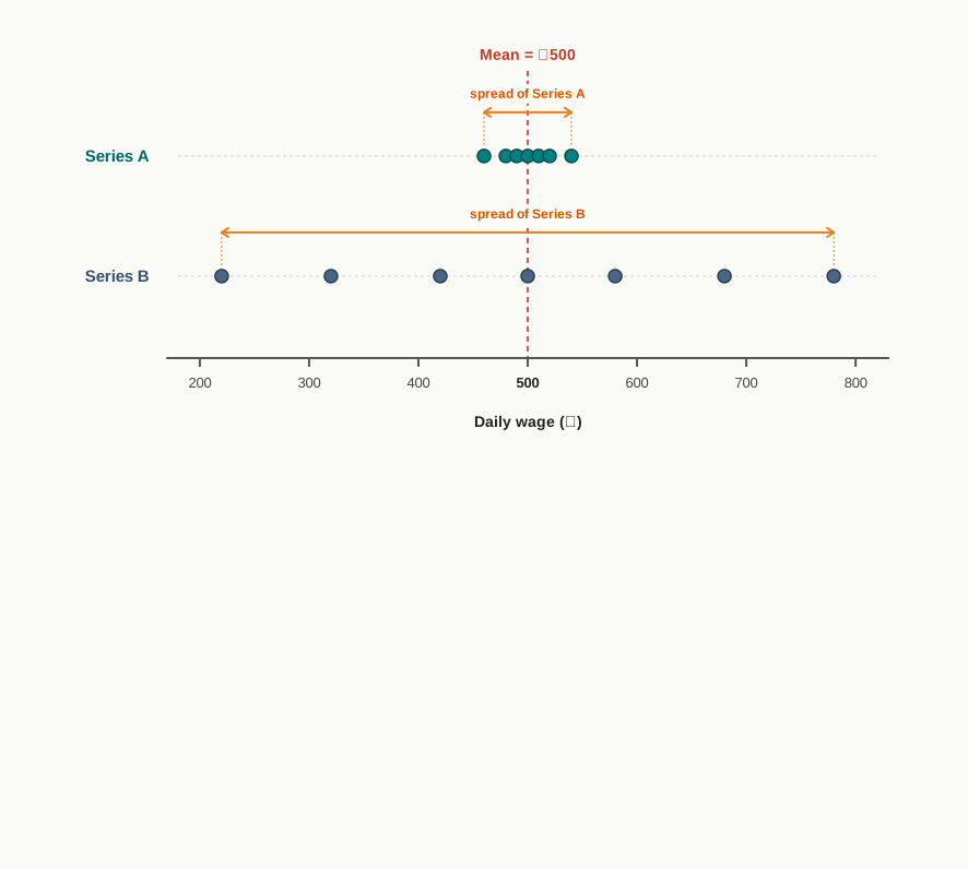
Fig. 19.0 – Two series with the same average but different spread.

19.1 The Need to Measure Dispersion

19.1.1 Why an Average Is Not Enough

A measure of central value condenses a large body of data into a single figure. That figure is representative in the sense that the observations cluster about it, and it allows two series to be compared at a glance. Statistics would be unmanageable without such condensation.

But condensation always costs information. The average records where the observations centre; it records nothing about how tightly or loosely they are gathered around that centre. Two series may share an average and yet describe quite different situations.

Suppose the number of children in four families is recorded in each of three colonies, as set out in Table 19.1. Every colony has twelve children in all, and so an average of three children per family.

Table

Table 19.1 — Number Of Children Per Family In Three Colonies | Family number | Colony X | Colony Y | Colony Z | |—|—|—|—| | 1 | 3 | 1 | 2 | | 2 | 3 | 2 | 1 | | 3 | 3 | 3 | 1 | | 4 | 3 | 6 | 8 | | Total number of children | 12 | 12 | 12 | | Average per family (total ÷ 4) | 3 | 3 | 3 |

The three averages are identical, but the three colonies are not. In Colony X every family has exactly three children, so the average describes each family perfectly. In Colony Y the families differ, though not greatly. In Colony Z one family has eight children while two have only one, and the average of three describes no family in the colony at all.

The average is therefore a reliable representative in Colony X and a poor one in Colony Z. Whether an average can be trusted depends on how far the individual observations lie from it — and that is a second and independent property of the data, which must be measured separately.

Watch Out

An average tells us where the observations centre. Dispersion tells us how far the observations lie from that centre. The two are separate properties, and both are needed.

19.1.2 Meaning of Dispersion

The scatter of the observations about the average is called dispersion, or variation. Where the observations lie close to the average, dispersion is low and the series is said to be uniform or homogeneous. Where they lie far from it, dispersion is high and the series is heterogeneous.

Definition

Dispersion Dispersion is the extent to which the values of a series are scattered about an average of the series, or differ among themselves.

Dispersion is thus a property of the whole set of observations, not of any one of them. It is always measured with reference to some average, and the measures studied in this chapter differ chiefly in which average they are measured from and how the distances from it are treated.

19.1.3 Objectives of Measuring Dispersion

Dispersion is measured for four main reasons.

To judge the reliability of the average — a low dispersion means the average is close to most of the observations and can be trusted to represent them, while a high dispersion warns that the average stands for very few of the items actually observed.
To describe the composition of a series — the average and the dispersion taken together tell us both where the data centre and how they are distributed about that centre, which neither figure conveys on its own.
To compare two or more series — two series with the same average may still differ in uniformity, and a comparison of averages alone would miss that difference entirely.
To control variation — once the extent of variation is measured, its causes can be investigated, and where variation is undesirable it can be reduced.

Exam Pointer

Questions on the objectives of dispersion expect the reliability of the average to be named first, with a reason. Stating the four objectives as bare labels, without explaining each in a line, does not earn full marks.

19.1.4 Usefulness of Dispersion

The study of dispersion has wide application in economics and in business.

Income and wealth — the extent of inequality in an economy is a question about the dispersion of incomes, since average income alone cannot show how unequally that income is shared.
Quality control — parts manufactured separately must be assembled later, so a producer needs the variation in their sizes to stay within narrow limits, whatever the average size may be.
Productivity — variation in output per worker across a workshop directs the manager’s attention to the causes of that variation rather than to the average alone.
Financial markets — the variability of the price of a share or a bond is taken as a measure of the risk carried by the person who holds it.
Further statistical work — correlation, regression and the theory of sampling all rest on measures of dispersion, so the study of dispersion is a step towards the techniques that follow it.

Economy Example

Why An Average Income Can Mislead Per capita income is a national average: total income divided by population. It says nothing about how that income is shared between rich and poor households, or between states. Two economies with the same per capita income can differ sharply in inequality. This is why measures of dispersion are studied alongside the average whenever the distribution of income is in question.

19.1.5 Properties of a Good Measure of Dispersion

Several measures of dispersion are in use, and they do not all serve equally well. A good measure should satisfy the following conditions.

Rigidly defined — the measure should be defined precisely, so that every person computing it from the same data arrives at the same value.
Easy to understand and simple to calculate — a measure that is laborious or obscure will not be used, however sound it may be in principle.
Based on all the observations — a measure that ignores most of the data cannot reflect the variation present in them.
Not unduly affected by extreme values — one unusually large or small observation should not be allowed to dominate the result.
Stable across samples — the measure should not vary widely between different samples drawn from the same population.
Capable of algebraic treatment — where the measure is known for two parts of a set of data, it should be possible to obtain the measure for the whole.

No single measure satisfies every one of these conditions. The merits and demerits of each measure, examined in the sections that follow, are best read as a record of which conditions it meets and which it fails.

19.2 Types of Measures of Dispersion

Dispersion can be measured in more than one way, and the measures fall into two families. The first states the scatter in the units in which the data themselves are recorded. The second states it as a ratio, free of any unit. The whole classification is set out in Fig. 19.1.

Fig. 19.1

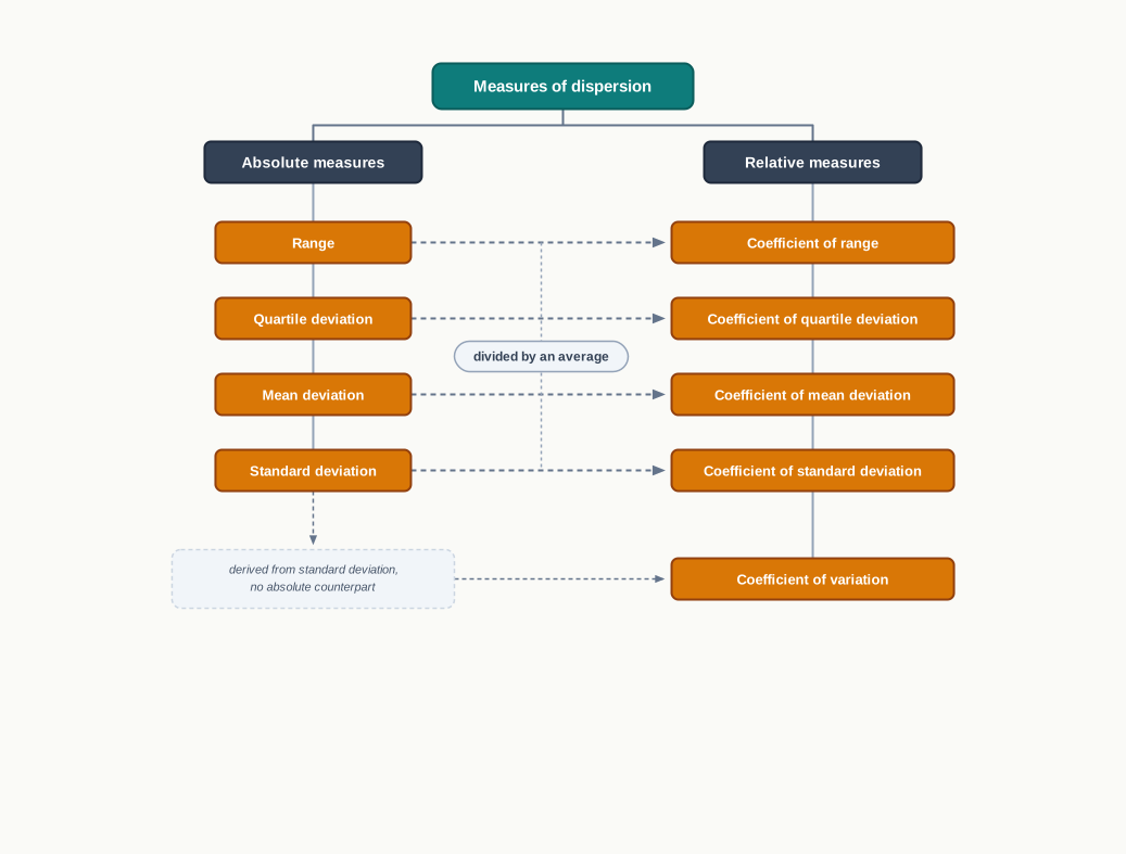
Fig. 19.1 – Classification of the measures of dispersion.

19.2.1 Absolute Measures of Dispersion

An absolute measure states the scatter in the same unit as the original data. If the data are daily wages in rupees, the measure is a number of rupees; if they are heights in centimetres, it is a number of centimetres.

Definition

Absolute Measure of Dispersion An absolute measure of dispersion expresses the variation of a series in the original units in which the data of the series are measured.

Because the unit survives the calculation, an absolute measure can be read directly and reported as it stands. It is the natural choice whenever a single distribution is under study and no comparison with another distribution is intended.

19.2.2 Relative Measures of Dispersion

The unit that makes an absolute measure easy to read also makes it useless for comparison. A scatter of ₹40 in the wages of one factory cannot be set against a scatter of 6 centimetres in the heights of its workers, because rupees and centimetres cannot be compared at all. Even two series in the same unit are not safely compared by an absolute measure if their averages are far apart: a variation of ₹5 means one thing in the price of a kilogram of onions and quite another in the price of a gram of gold.

The remedy is to divide the absolute measure by an average of the same series. The unit then cancels, and what remains is a pure number that can be set beside the corresponding figure for any other series.

\[\text{Relative measure of dispersion} = \dfrac{\text{Absolute measure of dispersion}}{\text{Average of the series}}\]

Here the absolute measure and the average are both in the units of the original data, so the ratio has no unit at all. A larger value means greater variation relative to the size of the observations themselves.

Definition

Relative Measure of Dispersion A relative measure of dispersion expresses the variation of a series as a ratio of an absolute measure to an average of that series. It is a pure number, independent of the units in which the data are measured.

A relative measure of dispersion is also called a coefficient of dispersion. Each of the four absolute measures has its own coefficient, and the coefficient of variation, taken up in §19.7, is a fifth relative measure obtained from the standard deviation.

The main points of difference are set out below.

Compare Table

Watch Out

A relative measure is not a different kind of scatter. It is the same scatter, divided by an average so that the unit cancels and comparison becomes possible.

19.2.3 Distance Measures and Average Deviation Measures

The four absolute measures divide again, this time by the method they use to arrive at a figure for the scatter.

Distance measures — these take the distance between two values in the series and treat that distance as the measure of the scatter. The larger the distance, the greater the variation. Range and quartile deviation are distance measures.
Average deviation measures — these find how far each observation lies from an average of the series, and then average those distances. Every observation contributes to the result. Mean deviation and standard deviation are average deviation measures.

The distinction matters because it explains the merits and demerits met later in the chapter. A distance measure is quick to compute but rests on two values only, so it ignores everything that lies between them. An average deviation measure uses the whole series and is correspondingly more representative, but it takes longer to compute and is more sensitive to observations lying far from the centre.

19.2.4 The Four Measures Studied in This Chapter

The syllabus requires four absolute measures, their coefficients, and the coefficient of variation. They are taken up in turn.

Range — the difference between the largest and the smallest observation in the series.
Quartile deviation — half the distance between the third quartile and the first quartile, so that it measures the spread of the middle half of the data.
Mean deviation — the average of the distances of the observations from the mean or from the median, the signs of those distances being ignored.
Standard deviation — the square root of the average of the squared distances of the observations from the arithmetic mean.

Each section defines the measure, works it out for individual, discrete and continuous series, gives its coefficient, and closes with its merits and demerits.

Exam Pointer

When a question asks for the difference between absolute and relative measures, the unit is the marking point. State that the absolute measure carries the unit of the data and the relative measure carries none.

19.3 Range

19.3.1 Meaning of Range

The simplest question that can be asked about the scatter of a series is how far apart its two extreme observations lie. The answer is the range.

Definition

Range Range is the difference between the highest and the lowest value observed in a series.

Range measures the total spread of the data from one end to the other. It states the width of the interval within which every observation of the series must fall, and says nothing about how the observations are distributed inside that interval.

\[R = H - L\]

Here \(R\) is the range, \(H\) the highest value observed in the series and \(L\) the lowest value observed. The result carries the unit of the original data, so the range of a wage series is in rupees and the range of a height series in centimetres. A larger value of \(R\) means a wider spread.

Fig. 19.2 shows what the measure captures and what it leaves out.

Fig. 19.2

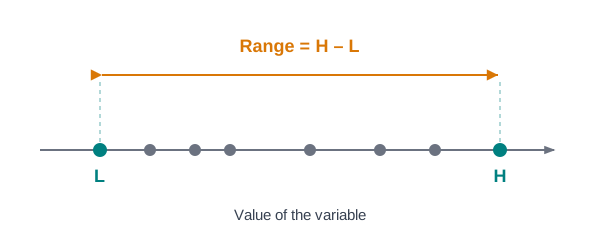
Fig. 19.2 – Range as the distance between the two extreme values.

19.3.2 Range in an Individual Series

In an individual series the observations are listed one by one. The largest and the smallest are read off directly and subtracted. Arranging the data in ascending order first is not strictly necessary, but it makes the two extreme values easy to identify and guards against error.

Example 19.1

SE 19.1 — Range Of An Individual Series

The daily earnings of eight street vendors in a market, in rupees, are 420, 380, 615, 290, 540, 460, 355 and 700. Calculate the range of daily earnings.

Arranged in ascending order: 290, 355, 380, 420, 460, 540, 615, 700

Highest value \(H = ₹700\)

Lowest value \(L = ₹290\)

\(R = H - L = 700 - 290 = ₹410\)

The daily earnings of the eight vendors are spread over an interval of ₹410.

19.3.3 Range in a Discrete Series

A discrete series records each value of the variable along with the number of times it occurs. The range is found exactly as in an individual series: the smallest value of the variable is subtracted from the largest. The frequencies are not used at all, because the range is a statement about which values occur, not about how often they occur. The data of the following example are set out in Table 19.2.

Table

Table 19.2 — Number Of Members Per Household In A Locality | Number of members | 2 | 3 | 4 | 5 | 6 | 7 | 9 | |—|—|—|—|—|—|—|—| | Number of households | 8 | 14 | 26 | 31 | 17 | 6 | 2 |

Example 19.2

SE 19.2 — Range Of A Discrete Series

From the distribution of household size given in Table 19.2, calculate the range.

Highest value of the variable \(H = 9\) members

Lowest value of the variable \(L = 2\) members

\(R = H - L = 9 - 2 = 7\) members

Household size in the locality varies over an interval of 7 members. The frequencies, which show that most households have four or five members, play no part in the result.

Watch Out

In a discrete series the range is the difference between the largest and smallest values of the variable, never between the largest and smallest frequencies.

19.3.4 Range in a Continuous Series

In a continuous series the individual observations are lost inside class intervals, so the highest and lowest values are not directly available. Two methods are in use, and they do not give the same answer.

Method 1 — take the difference between the mid-value of the highest class and the mid-value of the lowest class.
Method 2 — take the difference between the upper class boundary of the highest class and the lower class boundary of the lowest class.

Method 1 treats the mid-value as representative of its class, which is the convention followed everywhere else in the treatment of grouped data. Method 2 takes the outer limits of the distribution and therefore always gives the larger figure, exceeding Method 1 by exactly one class width.

Where the classes are inclusive — that is, where one class ends at 249 and the next begins at 250 — the class boundaries must be found before Method 2 can be applied. The gap between the two classes is divided equally, half a unit being subtracted from the lower limit and added to the upper limit of each class. Method 1 needs no such conversion, since the mid-value of a class is unchanged by it. The distribution used below is set out in Table 19.3.

Table

Table 19.3 — Weekly Wages Of Workers In A Small Unit | Weekly wages (₹) | Number of workers | |—|—| | 200–249 | 6 | | 250–299 | 18 | | 300–349 | 34 | | 350–399 | 22 | | 400–449 | 10 | | Total | 90 |

Example 19.3

SE 19.3 — Range Of A Continuous Series By Both Methods

From the wage distribution given in Table 19.3, calculate the range by Method 1 and by Method 2.

Method 1

Mid-value of the highest class \(\dfrac{400 + 449}{2} = ₹424.5\)

Mid-value of the lowest class \(\dfrac{200 + 249}{2} = ₹224.5\)

\(R = 424.5 - 224.5 = ₹200\)

Method 2

The classes are inclusive, so they are first converted to class boundaries by subtracting 0.5 from each lower limit and adding 0.5 to each upper limit. The lowest class becomes 199.5–249.5 and the highest class becomes 399.5–449.5.

Upper boundary of the highest class \(₹449.5\)

Lower boundary of the lowest class \(₹199.5\)

\(R = 449.5 - 199.5 = ₹250\)

The two methods give ₹200 and ₹250, differing by one class width of ₹50. The method used must always be stated along with the answer.

Exam Pointer

For a continuous series, name the method before computing, since Method 1 and Method 2 give different answers and both are correct. Convert inclusive classes to boundaries only for Method 2 — mid-values are unaffected by the conversion.

19.3.5 Coefficient of Range

Range carries the unit of the data, so the ranges of two series cannot be compared unless the series are measured in the same unit and have averages of much the same size. The relative measure that removes this difficulty is the coefficient of range.

There is no average of the range itself to divide by, so the sum of the two extreme values is used in its place.

\[\text{Coefficient of range} = \dfrac{H - L}{H + L}\]

Here \(H\) and \(L\) are again the highest and lowest values of the series. Both numerator and denominator carry the same unit, so the coefficient is a pure number. It lies between 0 and 1, and the closer it is to 1, the greater the variation relative to the size of the observations themselves. The two series compared below are given in Table 19.4.

Table

Table 19.4 — Closing Prices Of Two Shares Over Six Trading Days (₹) | Trading day | Share A | Share B | |—|—|—| | 1 | 240 | 60 | | 2 | 250 | 74 | | 3 | 235 | 55 | | 4 | 260 | 80 | | 5 | 245 | 66 | | 6 | 255 | 70 |

Example 19.4

SE 19.4 — Comparing Two Series By The Coefficient Of Range

For the two shares whose closing prices are given in Table 19.4, calculate the range and the coefficient of range, and state which share showed the greater variation in price.

Share A

\(H = ₹260\), \(L = ₹235\)

\(R = 260 - 235 = ₹25\)

Coefficient of range \(= \dfrac{260 - 235}{260 + 235} = \dfrac{25}{495} = 0.05\)

Share B

\(H = ₹80\), \(L = ₹55\)

\(R = 80 - 55 = ₹25\)

Coefficient of range \(= \dfrac{80 - 55}{80 + 55} = \dfrac{25}{135} = 0.19\)

The absolute range is ₹25 for both shares, but the coefficient of range is 0.05 for Share A and 0.19 for Share B. Measured against the level of its own price, Share B varied nearly four times as much.

Economy Example

The Day’s Price Band In A Mandi Market reports for an agricultural commodity arriving at a regulated mandi routinely publish the lowest and the highest price at which the day’s lots were sold, alongside the modal price. The gap between those two figures is the range. It tells buyers and growers at once how widely quality and bargaining outcomes differed on that day, though it says nothing about the price most lots actually fetched.

19.3.6 Merits of Range

Easy to understand — the meaning of the largest value less the smallest is plain to anyone, which is why the range is the measure most often quoted outside statistics.
Simple to calculate — it needs only two observations and a single subtraction, and no average has to be found first.
Useful where the limits matter — in quality control, in the reporting of price and temperature movements, and in setting tolerance limits, it is precisely the outer bounds of the variation that are wanted.

19.3.7 Demerits of Range

Not rigidly defined — for a continuous series two accepted methods exist and give different answers, so the same data can yield more than one range.
Not based on all the observations — only the two extreme values enter the calculation, and the distribution of everything between them is ignored entirely.
Unduly affected by extreme values — a single unusually high or low observation raises the range sharply, though the rest of the series may be closely packed.
Unstable across samples — because it rests on two observations, the range differs widely between samples drawn from the same population.
Not applicable to open-ended distributions — where the first or last class has no stated limit, neither method can be applied.

These demerits are serious enough that the range is rarely used as the only measure of dispersion. It is best treated as a first, rough indication of spread, to be followed by a measure that takes the whole series into account.

19.4 Quartile Deviation

19.4.1 Quartiles and the Interquartile Range

The weakness of the range is that its two extreme values are exactly the observations least likely to be typical. A measure that ignores the outer portions of the data and reports the spread of the central portion instead escapes that weakness. The quartiles provide the dividing points.

Definition

Quartiles Quartiles are the three values which divide a series arranged in order of magnitude into four equal parts, each part containing one-fourth of the observations.

The three quartiles are written \(Q_1\), \(Q_2\) and \(Q_3\). The first quartile \(Q_1\), called the lower quartile, is the value below which one-fourth of the observations lie. The second quartile \(Q_2\) is the value below which one-half of them lie, and is therefore the median. The third quartile \(Q_3\), called the upper quartile, is the value below which three-fourths of the observations lie. Their position in the series is shown in Fig. 19.3.

Fig. 19.3

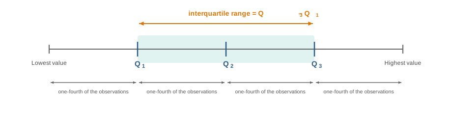
Fig. 19.3 – Quartiles dividing a series into four equal parts.

The distance between the upper and the lower quartile is the interquartile range.

\[\text{Interquartile range} = Q_3 - Q_1\]

Since one-fourth of the observations lie below \(Q_1\) and one-fourth above \(Q_3\), this distance spans the middle half of the series. It carries the unit of the original data, and a larger value means the central half of the observations is more widely spread.

19.4.2 Meaning of Quartile Deviation

The interquartile range measures the spread of half the observations, so halving it gives a figure comparable to a deviation on either side of the centre. That figure is the quartile deviation.

Definition

Quartile Deviation Quartile deviation is one-half of the difference between the third quartile and the first quartile of a series. It is also called the semi-interquartile range.

\[QD = \dfrac{Q_3 - Q_1}{2}\]

Here \(QD\) is the quartile deviation and \(Q_3\) and \(Q_1\) are the upper and lower quartiles. The result is in the units of the data. It is read as the average distance of the two quartiles from the median, so a quartile deviation of ₹40 says that the middle half of the series lies roughly within ₹40 on either side of the median.

Quartile deviation is a distance measure, like the range. It differs from the range in the two values whose distance it takes: not the extreme observations, but the two points that cut off the outer quarters of the data.

Watch Out

Quartile deviation is half the interquartile range, not the interquartile range itself. The difference \(Q_3 - Q_1\) is the interquartile range; dividing it by 2 gives the quartile deviation.

19.4.3 Quartile Deviation in an Individual Series

The observations are first arranged in ascending order. The positions of the two quartiles are then located by the following rules.

\[Q_1 = \text{size of } \left(\dfrac{N+1}{4}\right)\text{th item} \qquad Q_3 = \text{size of } \dfrac{3(N+1)}{4}\text{th item}\]

Here \(N\) is the number of observations. The two expressions give positions in the ordered array, not values: the value standing at that position is the quartile. Where the position works out to a whole number the value is read off directly, and where it is fractional the quartile lies between two adjacent observations and is estimated approximately.

Example 19.5

SE 19.5 — Quartile Deviation Of An Individual Series

The daily sales of eleven kirana shops in a neighbourhood, in hundreds of rupees, are 260, 380, 150, 420, 200, 340, 120, 300, 500, 180 and 240. Calculate the interquartile range and the quartile deviation.

Arranged in ascending order: 120, 150, 180, 200, 240, 260, 300, 340, 380, 420, 500

\(N = 11\)

Position of \(Q_1 = \dfrac{N+1}{4} = \dfrac{12}{4} = 3\)rd item

\(Q_1 = ₹180\) hundred

Position of \(Q_3 = \dfrac{3(N+1)}{4} = \dfrac{3 \times 12}{4} = 9\)th item

\(Q_3 = ₹380\) hundred

Interquartile range \(= Q_3 - Q_1 = 380 - 180 = ₹200\) hundred

\(QD = \dfrac{Q_3 - Q_1}{2} = \dfrac{200}{2} = ₹100\) hundred

The middle half of the shops record daily sales lying roughly within ₹100 hundred on either side of the median shop.

19.4.4 Quartile Deviation in a Discrete Series

In a discrete series the same positional formulas are used, with \(N\) taken as the total frequency \(\Sigma f\). The positions are located against a column of cumulative frequencies: the quartile is the value of the variable against the first cumulative frequency that equals or exceeds the required position. The cumulative frequencies for the following example are worked out in Table 19.5.

Table

Table 19.5 — Working For Quartile Deviation Of Overtime Hours Worked | Overtime hours in a week (X) | Number of workers (f) | Cumulative frequency (c.f.) | |—|—|—| | 2 | 5 | 5 | | 3 | 9 | 14 | | 4 | 14 | 28 | | 5 | 20 | 48 | | 6 | 16 | 64 | | 7 | 10 | 74 | | 8 | 5 | 79 | | Total | 79 | |

Example 19.6

SE 19.6 — Quartile Deviation Of A Discrete Series

Seventy-nine workers in a unit report the overtime hours they worked in a week. From the cumulative frequencies set out in Table 19.5, calculate the quartile deviation of overtime hours.

From Table 19.5, \(N = \Sigma f = 79\)

Position of \(Q_1 = \dfrac{N+1}{4} = \dfrac{80}{4} = 20\)th item

The first cumulative frequency equalling or exceeding 20 is 28, against 4 hours.

\(Q_1 = 4\) hours

Position of \(Q_3 = \dfrac{3(N+1)}{4} = \dfrac{3 \times 80}{4} = 60\)th item

The first cumulative frequency equalling or exceeding 60 is 64, against 6 hours.

\(Q_3 = 6\) hours

\(QD = \dfrac{Q_3 - Q_1}{2} = \dfrac{6 - 4}{2} = 1\) hour

The middle half of the workers put in between 4 and 6 hours of overtime, a quartile deviation of 1 hour.

Exam Pointer

Use \(\dfrac{N+1}{4}\) to locate the quartiles in individual and discrete series, but \(\dfrac{N}{4}\) in a continuous series. Marks are lost by carrying the \(N+1\) form into grouped data.

19.4.5 Quartile Deviation in a Continuous Series

In a continuous series the observations are grouped, so a quartile cannot be read off as the value of a particular item. The class in which the quartile falls is located first, and its value inside that class is then estimated by interpolation. Because the variable is treated as continuous, the positions are taken as the \(\dfrac{N}{4}\)th and \(\dfrac{3N}{4}\)th items rather than the \(\dfrac{N+1}{4}\)th and \(\dfrac{3(N+1)}{4}\)th.

\[Q_1 = l_1 + \dfrac{\dfrac{N}{4} - c.f.}{f} \times C \qquad Q_3 = l_1 + \dfrac{\dfrac{3N}{4} - c.f.}{f} \times C\]

Here \(l_1\) is the lower limit of the class in which the quartile lies, \(c.f.\) the cumulative frequency of the class preceding it, \(f\) the frequency of the quartile class itself, \(C\) the size of that class, and \(N\) the total frequency. The result carries the unit of the variable. The distribution and its cumulative frequencies are set out in Table 19.6.

Table

Table 19.6 — Working For Quartile Deviation Of Monthly Electricity Consumption | Consumption (units) | Number of households (f) | Cumulative frequency (c.f.) | |—|—|—| | 50–100 | 6 | 6 | | 100–150 | 12 | 18 | | 150–200 | 26 | 44 | | 200–250 | 20 | 64 | | 250–300 | 12 | 76 | | 300–350 | 4 | 80 | | Total | 80 | |

Example 19.7

SE 19.7 — Quartile Deviation Of A Continuous Series

The monthly electricity consumption of eighty households is recorded in Table 19.6, where the cumulative frequencies have also been worked out. Estimate the quartile deviation of consumption.

From Table 19.6, \(N = 80\)

\(\dfrac{N}{4} = \dfrac{80}{4} = 20\), which lies in the class 150–200, since the cumulative frequency reaches 44 in that class

For this class \(l_1 = 150\), \(c.f. = 18\), \(f = 26\), \(C = 50\)

\(Q_1 = 150 + \dfrac{20 - 18}{26} \times 50 = 150 + \dfrac{100}{26} = 150 + 3.85 = 153.85\) units

\(\dfrac{3N}{4} = \dfrac{3 \times 80}{4} = 60\), which lies in the class 200–250, since the cumulative frequency reaches 64 in that class

For this class \(l_1 = 200\), \(c.f. = 44\), \(f = 20\), \(C = 50\)

\(Q_3 = 200 + \dfrac{60 - 44}{20} \times 50 = 200 + \dfrac{800}{20} = 200 + 40 = 240\) units

\(QD = \dfrac{Q_3 - Q_1}{2} = \dfrac{240 - 153.85}{2} = \dfrac{86.15}{2} = 43.08\) units

The middle half of the households consume between 153.85 and 240 units a month, a quartile deviation of 43.08 units.

19.4.6 Coefficient of Quartile Deviation

Quartile deviation carries the unit of the data and cannot be compared across series measured differently. Dividing the interquartile range by the sum of the two quartiles removes the unit and gives the coefficient of quartile deviation.

\[\text{Coefficient of } QD = \dfrac{Q_3 - Q_1}{Q_3 + Q_1}\]

Here \(Q_3\) and \(Q_1\) are the two quartiles. Numerator and denominator carry the same unit, so the coefficient is a pure number lying between 0 and 1. The larger it is, the greater the variation in the central half of the data relative to the level of the observations.

Example 19.8

SE 19.8 — Coefficient Of Quartile Deviation

For the electricity consumption data of SE 19.7, in which \(Q_1 = 153.85\) units and \(Q_3 = 240\) units, calculate the coefficient of quartile deviation.

\(Q_3 - Q_1 = 240 - 153.85 = 86.15\) units

\(Q_3 + Q_1 = 240 + 153.85 = 393.85\) units

Coefficient of \(QD = \dfrac{86.15}{393.85} = 0.22\)

The coefficient of quartile deviation is 0.22, a pure number that can be set beside the corresponding figure for any other consumption or income series, whatever its unit.

Economy Example

Reading Income Data With An Open Top Class Income and consumption distributions published from household surveys usually end in an open class such as ‘above one lakh rupees a month’, because a few very large incomes would otherwise stretch the table. No highest value is available, so the range cannot be computed at all. Quartile deviation can, since it needs only the two quartiles, both of which lie well inside the closed classes.

19.4.7 Merits of Quartile Deviation

Simple to understand and calculate — it requires only the two quartiles, and no deviation has to be taken from an average.
Not affected by extreme values — the highest and lowest quarters of the data are set aside altogether, so an unusually large or small observation cannot influence the result.
Usable with open-ended distributions — the quartiles lie inside the closed classes, so the measure can be computed where range and standard deviation cannot.
Suited to the central portion of the data — where interest lies in how the typical half of a series is spread, it answers exactly that question.

19.4.8 Demerits of Quartile Deviation

Not rigidly defined — where the quartile position works out to a fraction, the quartile itself is only approximated, and different conventions yield slightly different values.
Not based on all the observations — it uses two values only and ignores the outer half of the data entirely, so it is less representative than a measure built from the whole series.
Unstable across samples — resting on two values, it differs from one sample to another drawn from the same population.
Not capable of algebraic treatment — quartile deviations of two parts of a set of data cannot be combined to give the quartile deviation of the whole.

Quartile deviation is therefore an improvement on the range, since it discards the extreme observations rather than depending on them, but it shares the range’s basic limitation of resting on two values only. A measure that uses every observation is taken up next.

19.5 Mean Deviation

19.5.1 Meaning of Mean Deviation

Range and quartile deviation each rest on two values. A measure that reflects the whole series must begin from every observation, and the natural way to do that is to ask how far each observation lies from the average and then to average those distances.

One difficulty appears at once. The deviations from the arithmetic mean are positive for observations above the mean and negative for those below it, and the two sets exactly cancel: the sum of the deviations from the arithmetic mean is always zero. Averaging them would give zero for every series, however scattered. Fig. 19.4 shows why.

Fig. 19.4

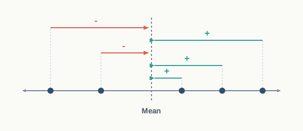
Fig. 19.4 – Deviations from the mean must be taken without signs.

The signs are accordingly dropped, and the absolute values of the deviations are averaged instead. The result is the mean deviation.

Definition

Mean Deviation Mean deviation is the arithmetic average of the absolute deviations of the observations of a series from the mean or the median of that series, the signs of the deviations being ignored.

Because the sign is discarded, mean deviation states how far a typical observation lies from the average, in either direction. It may be computed from the arithmetic mean or from the median, and the two give different answers, so the average used must always be stated. Of the two, the mean deviation taken from the median is the smaller.

Watch Out

Mean deviation from the mean and mean deviation from the median are two different figures. Always name the average the deviations were taken from when reporting the answer.

19.5.2 Mean Deviation in an Individual Series

Each observation’s distance from the chosen average is found, the signs are dropped, and the arithmetic mean of those distances is taken.

\[MD_{\bar{x}} = \dfrac{\Sigma |X - \bar{x}|}{N} \qquad MD_{m} = \dfrac{\Sigma |X - M|}{N}\]

Here \(X\) is an observation, \(\bar{x}\) the arithmetic mean, \(M\) the median, and \(N\) the number of observations. The vertical bars mean that the deviation is taken as a positive quantity whatever its sign. The result carries the unit of the original data. The deviations from both averages are worked out in Table 19.7.

Table

Table 19.7 — Working For Mean Deviation Of Monthly Expenditure On Books | Expenditure (₹) X | Deviation from mean |X – 400| | Deviation from median |X – 340| | |—|—|—| | 160 | 240 | 180 | | 200 | 200 | 140 | | 260 | 140 | 80 | | 300 | 100 | 40 | | 340 | 60 | 0 | | 420 | 20 | 80 | | 500 | 100 | 160 | | 560 | 160 | 220 | | 860 | 460 | 520 | | ΣX = 3,600 | Σ|X – 400| = 1,480 | Σ|X – 340| = 1,420 |

Example 19.9

SE 19.9 — Mean Deviation From The Mean, Individual Series

The monthly expenditure on books by nine students, in rupees, is 160, 200, 260, 300, 340, 420, 500, 560 and 860. Calculate the mean deviation from the arithmetic mean, the deviations being set out in Table 19.7.

\(N = 9\)

From Table 19.7, \(\Sigma X = 3{,}600\)

\(\bar{x} = \dfrac{\Sigma X}{N} = \dfrac{3{,}600}{9} = ₹400\)

From Table 19.7, \(\Sigma |X - \bar{x}| = 1{,}480\)

\(MD_{\bar{x}} = \dfrac{\Sigma |X - \bar{x}|}{N} = \dfrac{1{,}480}{9} = ₹164.44\)

A typical student’s expenditure lies about ₹164.44 away from the average expenditure of ₹400, in one direction or the other.

Example 19.10

SE 19.10 — Mean Deviation From The Median, Individual Series

For the same nine students of SE 19.9, calculate the mean deviation from the median, using the deviations already worked out in Table 19.7.

The data are already in ascending order and \(N = 9\)

Position of the median \(= \dfrac{N+1}{2} = \dfrac{10}{2} = 5\)th item

\(M = ₹340\)

From Table 19.7, \(\Sigma |X - M| = 1{,}420\)

\(MD_{m} = \dfrac{\Sigma |X - M|}{N} = \dfrac{1{,}420}{9} = ₹157.78\)

The mean deviation about the median is ₹157.78, smaller than the ₹164.44 obtained about the mean, as it always is.

19.5.3 Mean Deviation in a Discrete Series

Where each value occurs more than once, its deviation must count once for every occurrence. Each absolute deviation is therefore multiplied by the frequency of its value, and the total is divided by the total frequency.

\[MD_{\bar{x}} = \dfrac{\Sigma f|X - \bar{x}|}{\Sigma f} \qquad MD_{m} = \dfrac{\Sigma f|X - M|}{\Sigma f}\]

Here \(f\) is the frequency of the value \(X\), and the other symbols carry the meanings already given. The working for the following distribution is set out in Table 19.8.

Table

Table 19.8 — Working For Mean Deviation Of Marks Obtained | Marks (X) | Number of students (f) | fX | |X – 30| | f|X – 30| | |—|—|—|—|—| | 10 | 6 | 60 | 20 | 120 | | 20 | 10 | 200 | 10 | 100 | | 30 | 18 | 540 | 0 | 0 | | 40 | 10 | 400 | 10 | 100 | | 50 | 6 | 300 | 20 | 120 | | Total | Σf = 50 | ΣfX = 1,500 | | Σf|X – 30| = 440 |

Example 19.11

SE 19.11 — Mean Deviation From The Mean, Discrete Series

Fifty students appeared in a test marked out of 50. From the distribution and the working set out in Table 19.8, calculate the mean deviation from the arithmetic mean.

From Table 19.8, \(\Sigma f = 50\) and \(\Sigma fX = 1{,}500\)

\(\bar{x} = \dfrac{\Sigma fX}{\Sigma f} = \dfrac{1{,}500}{50} = 30 marks\)

From Table 19.8, \(\Sigma f|X - \bar{x}| = 440\)

\(MD_{\bar{x}} = \dfrac{\Sigma f|X - \bar{x}|}{\Sigma f} = \dfrac{440}{50} = 8.8 marks\)

A typical student’s score lies 8.8 marks away from the class average of 30 marks.

19.5.4 Mean Deviation in a Continuous Series

In a continuous series the individual observations are not available, so the mid-value of each class is taken to represent every observation in it. Beyond that substitution the procedure is exactly that of a discrete series.

\[MD_{\bar{x}} = \dfrac{\Sigma f|m - \bar{x}|}{\Sigma f}\]

Here \(m\) is the mid-value of a class and \(f\) its frequency. The arithmetic mean is itself computed from the mid-values as \(\bar{x} = \dfrac{\Sigma fm}{\Sigma f}\). The working is set out in Table 19.9.

Table

Table 19.9 — Working For Mean Deviation Of Daily Wages Of Casual Workers | Daily wages (₹) | Number of workers (f) | Mid-value (m) | fm | |m – 330| | f|m – 330| | |—|—|—|—|—|—| | 100–200 | 6 | 150 | 900 | 180 | 1,080 | | 200–300 | 14 | 250 | 3,500 | 80 | 1,120 | | 300–400 | 18 | 350 | 6,300 | 30 | 540 | | 400–500 | 8 | 450 | 3,600 | 120 | 960 | | 500–600 | 4 | 550 | 2,200 | 220 | 880 | | Total | Σf = 50 | | Σfm = 16,500 | | Σf|m – 330| = 4,580 |

Example 19.12

SE 19.12 — Mean Deviation And Its Coefficient, Continuous Series

The daily wages of fifty casual workers are distributed as shown in Table 19.9, where the mid-values and deviations have been worked out. Calculate the mean deviation from the arithmetic mean and its coefficient.

From Table 19.9, \(\Sigma f = 50\) and \(\Sigma fm = 16{,}500\)

\(\bar{x} = \dfrac{\Sigma fm}{\Sigma f} = \dfrac{16{,}500}{50} = ₹330\)

From Table 19.9, \(\Sigma f|m - \bar{x}| = 4{,}580\)

\(MD_{\bar{x}} = \dfrac{\Sigma f|m - \bar{x}|}{\Sigma f} = \dfrac{4{,}580}{50} = ₹91.60\)

Coefficient of \(MD = \dfrac{MD_{\bar{x}}}{\bar{x}} = \dfrac{91.60}{330} = 0.28\)

A typical worker’s daily wage lies ₹91.60 away from the average wage of ₹330, and the coefficient of 0.28 allows this variation to be compared with that of any other wage or income series.

Exam Pointer

Show the \(f|d|\) column and its total in the working table. Answers that jump from the frequency distribution to the final figure lose the method marks even when the answer is correct.

19.5.5 Coefficient of Mean Deviation

Mean deviation carries the unit of the data, so the relative measure is obtained by dividing it by the same average the deviations were taken from. This is the coefficient of mean deviation.

\[\text{Coefficient of } MD_{\bar{x}} = \dfrac{MD_{\bar{x}}}{\bar{x}} \qquad \text{Coefficient of } MD_{m} = \dfrac{MD_{m}}{M}\]

Here \(MD_{\bar{x}}\) and \(MD_{m}\) are the mean deviations from the mean and the median, and \(\bar{x}\) and \(M\) are those two averages. The unit cancels, leaving a pure number. The divisor must match the average used in computing the mean deviation: a mean deviation taken from the median is divided by the median, never by the mean.

Economy Example

Savings In A Self-Help Group A self-help group records the amount each member saves in a month. The average tells the group what a typical member contributes; the mean deviation tells it how far members usually depart from that figure. A small mean deviation means contributions are even and the group’s monthly pool is predictable. A large one warns that a few members carry the rest.

19.5.6 Merits of Mean Deviation

Based on all the observations — every item enters the calculation, so the measure reflects the whole series and not merely its extremes or its central half.
Simple to understand — it is the average distance from an average, which is exactly what the ordinary idea of scatter means.
Less affected by extreme values than standard deviation — the deviations are taken as they stand rather than squared, so an unusually distant observation does not dominate the result.
Flexible in the average used — it can be computed about the mean or about the median, whichever suits the data.

19.5.7 Demerits of Mean Deviation

Not well defined — since it may be taken from the mean or from the median, the same data yield more than one mean deviation, and the figure is meaningless unless the average used is stated.
Non-algebraic in nature — ignoring the signs of the deviations is a mathematical device rather than a sound operation, and it makes the measure unsuitable for further algebraic work.
Not capable of algebraic treatment — the mean deviations of two parts of a set of data cannot be combined to give the mean deviation of the whole.
Little used in advanced work — techniques such as correlation and regression are built on squared deviations, so mean deviation has no place in them.

Mean deviation therefore corrects the chief weakness of the two distance measures by using every observation, but it removes the signs of the deviations by discarding them. The measure taken up next removes them by squaring instead, and that single change makes it the most widely used measure of dispersion.

19.6 Standard Deviation

19.6.1 Meaning of Standard Deviation

Mean deviation disposed of the signs of the deviations by ignoring them. That works arithmetically but not algebraically, and it is the reason the measure leads nowhere beyond itself. There is a second way of removing a sign: squaring. The square of a negative number is positive, and squaring, unlike the dropping of a sign, is an operation that can be carried through the rest of a calculation.

Squaring the deviations, averaging the squares, and then taking the square root to return to the original unit gives the standard deviation.

Definition

Standard Deviation Standard deviation is the square root of the arithmetic mean of the squares of the deviations of the observations measured from the arithmetic mean of the series.

Standard deviation is always computed from the arithmetic mean, never from the median or the mode, so the ambiguity that troubles mean deviation does not arise. It is denoted by the Greek letter \(\sigma\), read sigma, and because it is the root of a mean of squares it is also called the root mean square deviation. The result carries the unit of the original data, and a larger \(\sigma\) means the observations lie further from their mean.

Economist

Karl Pearson Karl Pearson introduced the standard deviation and gave it the symbol \(\sigma\). Much of the statistical apparatus in ordinary use — the coefficient of correlation, the coefficient of variation and the methods built on squared deviations — descends from his work.

Watch Out

Standard deviation is taken from the arithmetic mean only. Unlike mean deviation, it has no version measured from the median, so no average needs to be named when reporting it.

19.6.2 Standard Deviation in an Individual Series

Two methods are in use. Both give the same answer; they differ only in the value the deviations are taken from.

19.6.2.1 Direct Method

The deviations are taken from the actual arithmetic mean.

\[\sigma = \sqrt{\dfrac{\Sigma x^2}{N}}\]

Here \(x = X - \bar{x}\) is the deviation of an observation from the arithmetic mean, \(\Sigma x^2\) the total of the squared deviations, and \(N\) the number of observations. The square root returns the answer to the unit of the original data. The working is set out in Table 19.10.

Table

Table 19.10 — Working For Standard Deviation Of Daily Sales By The Direct Method | Daily sales (₹ hundred) X | Deviation from mean x = X – 20 | Square of deviation x² | |—|—|—| | 13 | –7 | 49 | | 15 | –5 | 25 | | 19 | –1 | 1 | | 21 | +1 | 1 | | 25 | +5 | 25 | | 27 | +7 | 49 | | ΣX = 120 | Σx = 0 | Σx² = 150 |

Example 19.13

SE 19.13 — Standard Deviation By The Direct Method

The daily sales of a stationery shop over six days, in hundreds of rupees, are 13, 15, 19, 21, 25 and 27. Calculate the standard deviation, the working being set out in Table 19.10.

\(N = 6\)

From Table 19.10, \(\Sigma X = 120\)

\(\bar{x} = \dfrac{\Sigma X}{N} = \dfrac{120}{6} = ₹20\) hundred

From Table 19.10, \(\Sigma x^2 = 150\)

\(\sigma = \sqrt{\dfrac{\Sigma x^2}{N}} = \sqrt{\dfrac{150}{6}} = \sqrt{25} = ₹5\) hundred

Daily sales depart from their average of ₹20 hundred by ₹5 hundred in the root mean square sense.

19.6.2.2 Short-Cut Method

Where the arithmetic mean is not a whole number, deviations taken from it are awkward and every square becomes laborious. The short-cut method takes deviations from a convenient assumed mean instead, and corrects for the difference at the end.

\[\sigma = \sqrt{\dfrac{\Sigma d^2}{N} - \left(\dfrac{\Sigma d}{N}\right)^2}\]

Here \(d = X - A\) is the deviation of an observation from the assumed mean \(A\), which may be any value in or near the series. The term subtracted is the correction for the gap between the assumed mean and the true mean, and it is what makes the two methods agree. The working is set out in Table 19.11.

Table

Table 19.11 — Working For Standard Deviation Of Daily Sales By The Short-Cut Method | Daily sales (₹ hundred) X | Deviation from assumed mean d = X – 21 | Square of deviation d² | |—|—|—| | 13 | –8 | 64 | | 15 | –6 | 36 | | 19 | –2 | 4 | | 21 | 0 | 0 | | 25 | +4 | 16 | | 27 | +6 | 36 | | | Σd = –6 | Σd² = 156 |

Example 19.14

SE 19.14 — Standard Deviation By The Short-Cut Method

For the same six days of sales as in SE 19.13, calculate the standard deviation by the short-cut method, taking ₹21 hundred as the assumed mean. The working is set out in Table 19.11.

\(N = 6\), \(A = ₹21\) hundred

From Table 19.11, \(\Sigma d = -6\) and \(\Sigma d^2 = 156\)

\(\dfrac{\Sigma d^2}{N} = \dfrac{156}{6} = 26\)

\(\dfrac{\Sigma d}{N} = \dfrac{-6}{6} = -1\), and \(\left(\dfrac{\Sigma d}{N}\right)^2 = 1\)

\(\sigma = \sqrt{26 - 1} = \sqrt{25} = ₹5\) hundred

The answer is ₹5 hundred, exactly as by the direct method. The choice of assumed mean affects the working but never the result.

19.6.3 Standard Deviation in a Discrete Series

Each squared deviation is weighted by the frequency of its value, and the total is divided by the total frequency.

\[\sigma = \sqrt{\dfrac{\Sigma fx^2}{\Sigma f}}\]

Here \(f\) is the frequency of the value \(X\), \(x = X - \bar{x}\) the deviation of that value from the arithmetic mean, and \(\Sigma f = N\) the total frequency. The short-cut form for a discrete series replaces \(x\) by \(d = X - A\) and adds the same correction as before. The working is set out in Table 19.12.

Table

Table 19.12 — Working For Standard Deviation Of The Number Of Workers Per Small Unit | Workers per unit (X) | Number of units (f) | fX | x = X – 8 | x² | fx² | |—|—|—|—|—|—| | 4 | 2 | 8 | –4 | 16 | 32 | | 6 | 2 | 12 | –2 | 4 | 8 | | 8 | 12 | 96 | 0 | 0 | 0 | | 10 | 2 | 20 | +2 | 4 | 8 | | 12 | 2 | 24 | +4 | 16 | 32 | | Total | Σf = 20 | ΣfX = 160 | | | Σfx² = 80 |

Example 19.15

SE 19.15 — Standard Deviation Of A Discrete Series

Twenty small units in an industrial estate report the number of workers each employs. From the distribution and the working set out in Table 19.12, calculate the standard deviation.

From Table 19.12, \(\Sigma f = 20\) and \(\Sigma fX = 160\)

\(\bar{x} = \dfrac{\Sigma fX}{\Sigma f} = \dfrac{160}{20} = 8\) workers

From Table 19.12, \(\Sigma fx^2 = 80\)

\(\sigma = \sqrt{\dfrac{\Sigma fx^2}{\Sigma f}} = \sqrt{\dfrac{80}{20}} = \sqrt{4} = 2\) workers

Employment per unit departs from its average of 8 workers by 2 workers.

19.6.4 Standard Deviation in a Continuous Series

19.6.4.1 Direct and Short-Cut Methods

In a continuous series the mid-value of each class stands for every observation in it, and the two methods already given are applied to those mid-values.

\[\sigma = \sqrt{\dfrac{\Sigma fx^2}{N}} \qquad \sigma = \sqrt{\dfrac{\Sigma fd^2}{N} - \left(\dfrac{\Sigma fd}{N}\right)^2}\]

Here \(x = m - \bar{x}\) and \(d = m - A\), where \(m\) is the mid-value of a class, and \(N = \Sigma f\). Nothing else changes.

19.6.4.2 Step Deviation Method

Where the classes are of equal size, the deviations from the assumed mean are all multiples of the class size, and dividing them by it reduces every figure to a small whole number. This is the step deviation method, and it is the one ordinarily used for grouped data.

\[\sigma = \sqrt{\dfrac{\Sigma fd'^2}{N} - \left(\dfrac{\Sigma fd'}{N}\right)^2} \times C\]

Here \(d' = \dfrac{m - A}{C}\) is the step deviation, \(C\) the common class size, \(A\) the assumed mean and \(N = \Sigma f\). Dividing by \(C\) shrinks every deviation, so the final multiplication by \(C\) restores the answer to the unit of the original data. The arithmetic mean itself is obtained from the same columns as \(\bar{x} = A + \dfrac{\Sigma fd'}{N} \times C\). The working is set out in Table 19.13.

Table

Table 19.13 — Working For Standard Deviation Of Monthly Household Income By The Step Deviation Method | Monthly income (₹ thousand) | Number of households (f) | Mid-value (m) | d′ = (m – 35) ÷ 10 | fd′ | fd′² | |—|—|—|—|—|—| | 10–20 | 8 | 15 | –2 | –16 | 32 | | 20–30 | 14 | 25 | –1 | –14 | 14 | | 30–40 | 20 | 35 | 0 | 0 | 0 | | 40–50 | 12 | 45 | +1 | +12 | 12 | | 50–60 | 6 | 55 | +2 | +12 | 24 | | Total | Σf = 60 | | | Σfd′ = –6 | Σfd′² = 82 |

Example 19.16

SE 19.16 — Standard Deviation And Its Coefficient By The Step Deviation Method

The monthly incomes of sixty households are distributed as shown in Table 19.13, where the step deviations have been worked out about an assumed mean of ₹35 thousand. Calculate the arithmetic mean, the standard deviation and the coefficient of standard deviation.

From Table 19.13, \(N = \Sigma f = 60\), \(\Sigma fd' = -6\), \(\Sigma fd'^2 = 82\), with \(A = 35\) and \(C = 10\)

\(\bar{x} = A + \dfrac{\Sigma fd'}{N} \times C = 35 + \dfrac{-6}{60} \times 10 = 35 - 1 = ₹34\) thousand

\(\dfrac{\Sigma fd'^2}{N} = \dfrac{82}{60} = 1.3667\)

\(\left(\dfrac{\Sigma fd'}{N}\right)^2 = \left(\dfrac{-6}{60}\right)^2 = 0.01\)

\(\sigma = \sqrt{1.3667 - 0.01} \times 10 = \sqrt{1.3567} \times 10 = 1.165 \times 10 = ₹11.65\) thousand

Coefficient of \(SD = \dfrac{\sigma}{\bar{x}} = \dfrac{11.65}{34} = 0.34\)

Monthly incomes depart from their average of ₹34 thousand by ₹11.65 thousand, and the coefficient of 0.34 states that variation as a pure number.

Exam Pointer

In the step deviation method the final multiplication by the class size \(C\) is the step most often forgotten. Check the answer against the data: a standard deviation smaller than one class width almost always means \(C\) was left out.

19.6.5 Coefficient of Standard Deviation

Standard deviation carries the unit of the data. Dividing it by the arithmetic mean of the same series removes the unit and gives the coefficient of standard deviation.

\[\text{Coefficient of } SD = \dfrac{\sigma}{\bar{x}}\]

Here \(\sigma\) is the standard deviation and \(\bar{x}\) the arithmetic mean. Both carry the same unit, so the coefficient is a pure number, and the larger it is, the greater the variation relative to the size of the observations. Expressed as a percentage, this same ratio becomes the coefficient of variation, taken up in §19.7.

19.6.6 Merits of Standard Deviation

Rigidly defined — it is computed from the arithmetic mean by one method only, so the same data always yield the same value.
Based on all the observations — every item contributes a squared deviation, and the measure therefore reflects the whole series.
Capable of algebraic treatment — standard deviations of two parts of a set of data can be combined to give the standard deviation of the whole, which no other measure in this chapter permits.
Stable across samples — it is affected less by sampling fluctuations than the range or the quartile deviation.
Basis of further statistical work — correlation, regression and the theory of sampling all rest on it, so it is the measure that leads somewhere beyond itself.

19.6.7 Demerits of Standard Deviation

Difficult to compute — squaring every deviation and extracting a root make it the most laborious of the four measures, and the least easily explained to a reader without training.
Gives more weight to extreme values — squaring magnifies the large deviations more than the small ones, so an observation far from the mean influences the result out of proportion to its number.

These two demerits are real but slight beside the merits. Standard deviation is accordingly the measure of dispersion in ordinary use wherever the data allow it to be computed.

19.7 Coefficient of Variation

19.7.1 Meaning of the Coefficient of Variation

Standard deviation is the most satisfactory of the absolute measures, but it carries the unit of the data and so cannot be set against the standard deviation of a series measured differently. Even two series in the same unit are not safely compared by it if their averages are far apart, since a scatter of ₹50 means one thing about a wage of ₹200 and quite another about a wage of ₹2,000.

The coefficient of standard deviation, met in §19.6.5, removes the unit by dividing \(\sigma\) by the mean. Multiplying that ratio by 100 expresses it as a percentage, and the result is the coefficient of variation.

Definition

Coefficient of Variation Coefficient of variation is the ratio of the standard deviation of a series to its arithmetic mean, expressed as a percentage.

\[CV = \dfrac{\sigma}{\bar{x}} \times 100\]

Here \(\sigma\) is the standard deviation of the series and \(\bar{x}\) its arithmetic mean. The two carry the same unit, which cancels, so the coefficient of variation is a pure number stated in per cent. It says how large the scatter is as a proportion of the average about which that scatter occurs.

A high coefficient of variation means the observations are widely spread relative to their own average: the series is variable, unstable, and its average is a weak representative of it. A low coefficient means the observations cluster closely about their average: the series is consistent, stable and uniform, and its average can be trusted.

Watch Out

A higher coefficient of variation means greater variability and therefore less consistency. The series with the lower coefficient is the more consistent, uniform or stable of the two.

Example 19.17

SE 19.17 — Coefficient Of Variation Of A Single Series

The daily wages paid by a firm have an arithmetic mean of ₹450 and a standard deviation of ₹63. Calculate the coefficient of variation.

\(\bar{x} = ₹450\), \(\sigma = ₹63\)

\(CV = \dfrac{\sigma}{\bar{x}} \times 100 = \dfrac{63}{450} \times 100 = 14\) per cent

The scatter of daily wages is 14 per cent of the average wage, so wages in this firm are fairly uniform.

19.7.2 Comparing the Variability of Two Series

The coefficient of variation earns its place when two series must be compared. Because it is a pure number, the comparison holds whether the two series are measured in the same unit or in different ones, and whatever the gap between their averages.

The conclusion drawn from it can differ from the conclusion the standard deviations alone would suggest. A series with the larger standard deviation may still be the more consistent of the two, if its average is larger in proportion. The working for the following comparison is set out in Table 19.14.

Table

Table 19.14 — Working For The Coefficients Of Variation Of Two Workers’ Daily Output | Worker A output (units) | x = X – 20 | x² | Worker B output (units) | x = X – 30 | x² | |—|—|—|—|—|—| | 18 | –2 | 4 | 30 | 0 | 0 | | 20 | 0 | 0 | 25 | –5 | 25 | | 22 | +2 | 4 | 35 | +5 | 25 | | 24 | +4 | 16 | 32 | +2 | 4 | | 16 | –4 | 16 | 28 | –2 | 4 | | ΣX = 100 | | Σx² = 40 | ΣX = 150 | | Σx² = 58 |

Example 19.18

SE 19.18 — Comparing The Consistency Of Two Workers

The daily output of two workers over five days is recorded in Table 19.14, where the deviations from their respective means have been worked out. Determine which worker is the more consistent.

Worker A

\(N = 5\); from Table 19.14, \(\Sigma X = 100\) and \(\Sigma x^2 = 40\)

\(\bar{x} = \dfrac{100}{5} = 20\) units

\(\sigma = \sqrt{\dfrac{40}{5}} = \sqrt{8} = 2.83\) units

\(CV = \dfrac{2.83}{20} \times 100 = 14.15\) per cent

Worker B

\(N = 5\); from Table 19.14, \(\Sigma X = 150\) and \(\Sigma x^2 = 58\)

\(\bar{x} = \dfrac{150}{5} = 30\) units

\(\sigma = \sqrt{\dfrac{58}{5}} = \sqrt{11.6} = 3.41\) units

\(CV = \dfrac{3.41}{30} \times 100 = 11.37\) per cent

Worker B has the larger standard deviation, 3.41 units against 2.83, but the smaller coefficient of variation, 11.37 per cent against 14.15. Measured against his own higher average output, Worker B is the more consistent of the two.

Where the two series are measured in different units, the standard deviations cannot be compared at all and the coefficient of variation is the only measure available.

Example 19.19

SE 19.19 — Comparing Two Series Measured In Different Units

The monthly wage bill of a workshop has a mean of ₹480 thousand with a standard deviation of ₹72 thousand. Its monthly output has a mean of 60 quintals with a standard deviation of 12 quintals. State which of the two varies more.

Wage bill

\(CV = \dfrac{72}{480} \times 100 = 15\) per cent

Output

\(CV = \dfrac{12}{60} \times 100 = 20\) per cent

Rupees and quintals cannot be compared, but 15 per cent and 20 per cent can. Output varies more than the wage bill, at 20 per cent against 15 per cent.

Exam Pointer

End every comparison with a sentence naming the more consistent series and the two percentages. A question asking which series is more stable is not answered by the two coefficients alone.

Economy Example

Which Crop Gives The Steadier Income Agricultural economists compare crops by the coefficient of variation of their yields across a run of years. A crop with a high average yield but a high coefficient is a gamble: good years are very good and bad years ruinous. A crop with a lower average and a low coefficient offers a steadier income, which matters more to a cultivator with no cushion against a bad season.

19.8 Choosing a Measure of Dispersion

Four measures of dispersion have been worked out on the same kinds of data, and they do not agree with one another. That is not a defect. Each answers a slightly different question about the scatter, and the properties set out in §19.1.5 are met by each of them only in part. Choosing between them means knowing which properties matter for the work in hand.

19.8.1 Range and Quartile Deviation Compared

Both are distance measures: each takes two values from the series and reports the gap between them. They differ in which two values they take, and everything else follows from that. The main points of difference are set out below.

Compare Table

Quartile deviation is thus the better measure of the two wherever the extreme observations are unreliable, unrepresentative or simply missing. Range remains useful where the extremes are precisely what is wanted, as in quality control or in reporting the day’s highest and lowest price.

19.8.2 Mean Deviation and Standard Deviation Compared

Both are average deviation measures: each finds how far the observations lie from an average and then averages those distances. They differ in how the signs of the deviations are disposed of, and that single difference accounts for the standing of the two measures.

Compare Table

Standard deviation is accordingly the measure used wherever the data permit. Mean deviation survives as the simpler and more directly intelligible of the two, and as the measure less distorted by an observation lying far from the centre.

Watch Out

The coefficient of standard deviation and the coefficient of variation are the same ratio, \(\sigma \div \bar{x}\). The coefficient of variation is that ratio expressed as a percentage.

19.8.3 Which Measure to Use

No measure is best in the abstract. The choice turns on three questions: what the data allow, what degree of accuracy the purpose demands, and whether one series or two are being examined.

What the data allow — an open-ended distribution rules out range and standard deviation alike, leaving quartile deviation as the practical choice. Where the extreme observations are known to be unreliable, the same reasoning applies.
What the purpose demands — a rough indication of spread, wanted quickly, is served by the range. Any measure meant to represent the series properly must be built from all the observations, which narrows the choice to mean deviation and standard deviation.
Whether a comparison is intended — one series is described by an absolute measure. Two series measured in different units, or with very different averages, must be compared by a relative measure, and the coefficient of variation is the one ordinarily used.

The four measures and their relative counterparts are collected in Table 19.15.

Table

Table 19.15 — The Measures Of Dispersion And Their Coefficients | Measure | Absolute measure | Relative measure | |—|—|—| | Range | \(R = H - L\) | \(\dfrac{H - L}{H + L}\) | | Quartile deviation | \(QD = \dfrac{Q_3 - Q_1}{2}\) | \(\dfrac{Q_3 - Q_1}{Q_3 + Q_1}\) | | Mean deviation | \(MD = \dfrac{\Sigma f\lvert d \rvert}{\Sigma f}\) | \(\dfrac{MD}{\text{average used}}\) | | Standard deviation | \(\sigma = \sqrt{\dfrac{\Sigma fx^2}{\Sigma f}}\) | \(\dfrac{\sigma}{\bar{x}}\), or \(\dfrac{\sigma}{\bar{x}} \times 100\) as the coefficient of variation |

Exam Pointer

Questions asking you to distinguish between two measures expect basis-wise differences, not a paragraph. Give four bases, and close by naming which of the two is the more satisfactory and why.

Economy Example

Judging A Supplier’s Reliability A firm choosing between two suppliers records how many days each takes to deliver. The range shows the worst delay either has caused, which matters if a single late consignment halts production. The coefficient of variation shows which supplier is steadier overall, relative to its own average delivery time. The two figures answer different questions, and a buyer normally wants both.

19.9 Summary

A measure of central value tells us where a series centres, but nothing about how closely the observations gather around that centre. Two series may share an average and still differ entirely in their spread, which is why dispersion must be measured alongside the average.
Dispersion is the extent to which the values of a series are scattered about an average of the series, or differ among themselves. It is measured to judge how far the average may be trusted, to describe the composition of a series, to compare two series, and to control variation where variation is undesirable.
A good measure of dispersion should be rigidly defined, easy to understand and calculate, based on all the observations, unaffected by extreme values, stable across samples, and capable of algebraic treatment. No single measure satisfies all six conditions.
Measures of dispersion are of two kinds.
1. An absolute measure states the scatter in the original units of the data, and is used to describe a single series.
2. A relative measure, or coefficient of dispersion, is an absolute measure divided by an average of the same series. It is a pure number and is used to compare two or more series.
The absolute measures divide again by method. Range and quartile deviation are distance measures, taking the gap between two values. Mean deviation and standard deviation are average deviation measures, averaging the distances of all the observations from an average.
Range is the difference between the highest and lowest value observed, \(R = H - L\), where \(H\) is the highest and \(L\) the lowest value. Its relative measure is the coefficient of range, \(\dfrac{H - L}{H + L}\), a pure number lying between 0 and 1.
1. In a continuous series two methods are accepted — the difference of the mid-values of the highest and lowest classes, and the difference of the upper boundary of the highest class and the lower boundary of the lowest. The second always exceeds the first by one class width, so the method used must be stated.
2. Range is simple and useful where the outer limits matter, but it rests on two values only, is dominated by extreme observations, and cannot be computed for an open-ended distribution.
Quartiles divide an ordered series into four equal parts. Quartile deviation is half the distance between the upper and lower quartiles, \(QD = \dfrac{Q_3 - Q_1}{2}\), where \(Q_3\) and \(Q_1\) are the upper and lower quartiles; the undivided difference \(Q_3 - Q_1\) is the interquartile range. Its coefficient is \(\dfrac{Q_3 - Q_1}{Q_3 + Q_1}\).
1. In individual and discrete series the quartiles stand at the \(\left(\dfrac{N+1}{4}\right)\)th and \(\dfrac{3(N+1)}{4}\)th items, where \(N\) is the number of observations or the total frequency.
2. In a continuous series they are found by interpolation, \(Q_1 = l_1 + \dfrac{\dfrac{N}{4} - c.f.}{f} \times C\) and \(Q_3 = l_1 + \dfrac{\dfrac{3N}{4} - c.f.}{f} \times C\), where \(l_1\) is the lower limit of the quartile class, \(c.f.\) the cumulative frequency of the class before it, \(f\) its frequency and \(C\) its size.
3. Quartile deviation ignores the outer quarters of the data, so it is unaffected by extreme values and can be computed for open-ended distributions, but it still rests on two values only.
The deviations from the arithmetic mean always sum to zero, so their signs must be removed before they can be averaged. Mean deviation removes them by ignoring them; standard deviation removes them by squaring.
Mean deviation is the arithmetic average of the absolute deviations of the observations from the mean or the median, \(MD_{\bar{x}} = \dfrac{\Sigma f|X - \bar{x}|}{\Sigma f}\) and \(MD_{m} = \dfrac{\Sigma f|X - M|}{\Sigma f}\), where \(X\) is an observation, \(f\) its frequency, \(\bar{x}\) the arithmetic mean and \(M\) the median. In an individual series the frequencies drop out and the divisor is \(N\).
1. Its coefficient is the mean deviation divided by the same average it was taken from — \(\dfrac{MD_{\bar{x}}}{\bar{x}}\) or \(\dfrac{MD_{m}}{M}\).
2. The mean deviation about the median is always the smaller of the two, since the median makes the total of the absolute deviations as small as it can be.
3. It uses every observation, but ignoring signs is not a sound algebraic operation, and the measure leads no further.
Standard deviation is the square root of the arithmetic mean of the squared deviations from the arithmetic mean, and is written \(\sigma\). It is computed from the arithmetic mean alone.

Direct method — \(\sigma = \sqrt{\dfrac{\Sigma f x^2}{N}}\), where \(x = X - \bar{x}\) is the deviation from the actual mean and \(N\) the number of observations or the total frequency.
Short-cut method — \(\sigma = \sqrt{\dfrac{\Sigma f d^2}{N} - \left(\dfrac{\Sigma f d}{N}\right)^2}\), where \(d = X - A\) is the deviation from an assumed mean \(A\), the subtracted term correcting for the gap between \(A\) and the true mean.
Step deviation method — \(\sigma = \sqrt{\dfrac{\Sigma f d'^2}{N} - \left(\dfrac{\Sigma f d'}{N}\right)^2} \times C\), where \(d' = \dfrac{m - A}{C}\), \(m\) is the mid-value of a class and \(C\) the common class size. The final multiplication by \(C\) restores the answer to the unit of the data.
All three methods give the same answer for the same data, and the choice of assumed mean never affects the result.

The coefficient of standard deviation is \(\dfrac{\sigma}{\bar{x}}\). Expressed as a percentage, the same ratio is the coefficient of variation, \(CV = \dfrac{\sigma}{\bar{x}} \times 100\), where \(\sigma\) is the standard deviation and \(\bar{x}\) the arithmetic mean. A higher coefficient of variation means greater variability and therefore less consistency, and the comparison holds even between series measured in different units.
Standard deviation is rigidly defined, based on all the observations and capable of algebraic treatment, which makes it the measure ordinarily used and the foundation of correlation, regression and sampling theory. Its demerits are that it is laborious to compute and that squaring gives extreme observations disproportionate weight.
The choice of measure turns on what the data allow, what the purpose demands, and whether a comparison is intended. Open-ended classes or unreliable extremes point to quartile deviation; a quick rough answer point to range; a properly representative figure points to standard deviation; and a comparison across units or averages requires the coefficient of variation.

19.10 Points to Ponder

An economy reports a rising average income year after year, while the dispersion of incomes widens at the same time. Has that economy improved? What would you need to know before answering, and which of the two figures would you put first in a report?
Standard deviation squares the deviations, so an observation lying far from the mean counts for much more than one lying close to it. Where variation stands for risk — in the price of a share, or in the yield of a crop — is that extra weight a defect of the measure or exactly what is wanted?
Quartile deviation sets aside the highest and lowest quarters of the data before measuring anything. When is discarding observations a sound response to unreliable extremes, and when is it a convenient way of removing the very cases a study ought to be about?
Two workers are compared. One has the smaller standard deviation, the other the smaller coefficient of variation. If a firm must promote one of them for consistency, which figure should decide, and does the answer change if the two work in different departments producing different things?
Suppose the wages in a firm had zero dispersion, every worker earning exactly the average. Would that be a desirable state of affairs, and what would it imply about how the firm rewards effort, skill and experience?
Range is the least satisfactory measure by almost every property listed in this chapter, yet it is the one most often quoted in newspapers, market reports and weather bulletins. Why do simple measures survive their own defects, and what does the public use of a measure tell us that its statistical properties do not?

19.11 Objective Questions

Which of the following measures of dispersion is not affected by the extreme values of a series? [1]
1. Range
2. Quartile deviation
3. Standard deviation
4. Coefficient of variation
Assertion (A): The coefficient of variation is a pure number carrying no unit. Reason (R): It is obtained by dividing the standard deviation of a series by its arithmetic mean, so the unit of the data cancels. [1]
1. Both A and R are true and R is the correct explanation of A.
2. Both A and R are true but R is not the correct explanation of A.
3. A is true but R is false.
4. A is false but R is true.
Fill in the blank: The difference between the upper quartile and the lower quartile of a series is called the ______. [1]
State whether the following statement is true or false: Two series having the same standard deviation must also have the same coefficient of variation. [1]
Match the measure in Column I with its description in Column II. [1]

Column I	Column II
a. Quartile deviation	i. \(\dfrac{\sigma}{\bar{x}} \times 100\)
b. Coefficient of variation	ii. Also called the semi-interquartile range
c. Step deviation method	iii. Used to find the standard deviation of a continuous series with equal class intervals

19.12 Check Your Concepts

State any two differences between an absolute measure and a relative measure of dispersion. [2]
The marks obtained by five students in a test are 12, 15, 18, 21 and 24. Calculate the range and the coefficient of range. [3]
The daily wages of five workers, in hundreds of rupees, are 25, 30, 35, 40 and 45. Calculate the standard deviation by the direct method and the coefficient of variation. [4]
The monthly savings of fifty households, in hundreds of rupees, are distributed as follows: 0–10, five households; 10–20, ten households; 20–30, twenty households; 30–40, ten households; 40–50, five households. Estimate the quartile deviation and its coefficient. [6]

19.13 Case-Based Question

Ravi Malhotra runs a small garment unit and buys yarn from two suppliers. Over the past year, Sunrise Traders has taken an average of 12 days to deliver an order, with a standard deviation of 3 days. Deccan Yarns has taken an average of 20 days, with a standard deviation of 4 days. Ravi is inclined to call Sunrise Traders the steadier supplier because its deliveries vary by fewer days.
1. Calculate the coefficient of variation of delivery time for each supplier. [2]
2. State which supplier is the more consistent, and explain why a comparison of the two standard deviations alone would have misled Ravi. [2]