Chapter 22: Some Mathematical Tools Used in Economics
Every month a household receives an electricity bill built up in two parts: a fixed charge payable whether or not a single unit is consumed, and a further amount charged for each unit actually used. Two numbers — units consumed and the amount payable — move together in a settled way, so that once the fixed charge and the rate per unit are known, the bill for any level of consumption can be worked out in advance. Economics is full of relationships of this kind. Output depends on the number of workers employed, consumption expenditure depends on income, and quantity demanded depends on price. Earlier chapters expressed such relationships through schedules and through graphs; this chapter adds a third way of expressing them, the mathematical equation, and shows that the three are only different presentations of the same relationship. The chapter builds the vocabulary this requires: what a function is, how a relationship in which one variable changes at a constant rate is written as the equation of a straight line, what the intercept and the slope of that line stand for, and how a slope is measured and read from a graph. It covers functions and the equation of a line, and the slope of a straight line.
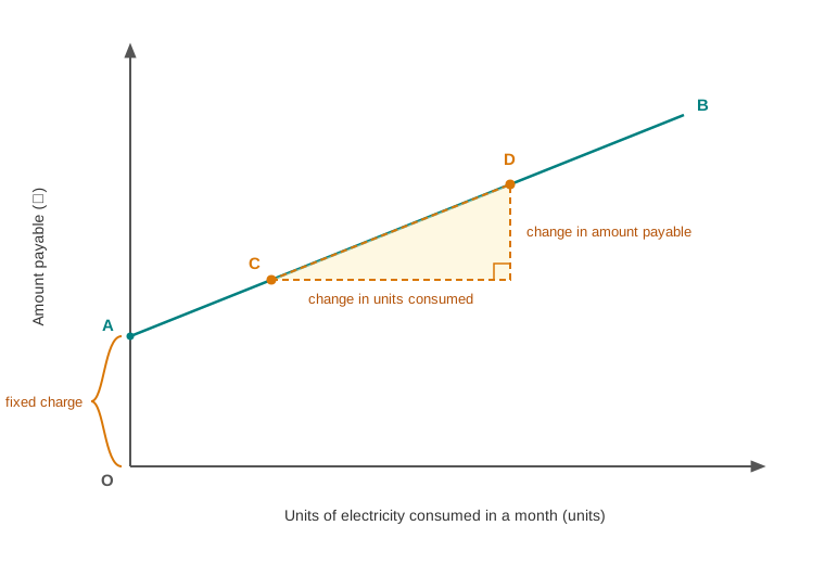
Fig. 22.0 – The electricity bill as a straight line.
22.1 Relationships Between Economic Variables
Economics deals with quantities that do not stand still. Prices rise and fall, incomes grow, output expands, employment contracts, and the general price level drifts upward year after year. A subject built on scarcity and choice has to keep track of such movement, because every choice an economy makes shows up as a change in some measurable quantity.
More than that, these quantities move together. A household that earns more usually saves more. A farm that employs more workers usually harvests more. A commodity whose price rises is usually bought in smaller quantities. Economics is interested less in a single quantity taken alone than in the settled way two quantities move in relation to each other.
Once such a relationship is known, it can be used. It allows the economist to say what saving would be at a level of income not yet reached, or what output would be if two more workers were employed. This section looks at what these changing quantities are, and at the three ways in which a relationship between two of them can be presented.
22.1.1 Variables in Economics
A quantity that can take different values is called a variable. Price is a variable because it can be ₹20 today and ₹24 next month. Quantity demanded, income, saving, consumption expenditure, output, employment and the price index are all variables, since each is capable of taking more than one value.
A quantity whose value does not change is a constant. The number of paise in a rupee is a constant, and so is a fixed licence fee that a trader pays whatever the volume of business done. A constant may appear inside a relationship without itself varying — the fixed charge in a bill is a constant even though the total bill is a variable.
Variables in economics are usually measured in definite units, and the unit must always be stated. Quantity may be in kilograms, litres or dozens; income and expenditure in rupees; employment in numbers of workers; and a price index in index points. A statement that output rose from 40 to 55 says nothing until the unit is known.
22.1.2 Schedules and Graphs as Ways of Showing a Relationship
The simplest way of presenting a relationship is to list paired values in a table. A table that sets out the value taken by one variable against each value of another is called a schedule. Table 22.1 gives the monthly saving of a household at four different levels of monthly income.
Two things can be read off the schedule at once. Saving rises as income rises, so the two variables move in the same direction. And every rise of ₹5,000 in income is accompanied by a rise of exactly ₹1,000 in saving, so the two move together at a steady rate.
The same information can be presented as a graph. Income is measured along one axis and saving along the other, each pair in the schedule is plotted as a point, and the points are joined. The result is shown in Fig. 22.1.
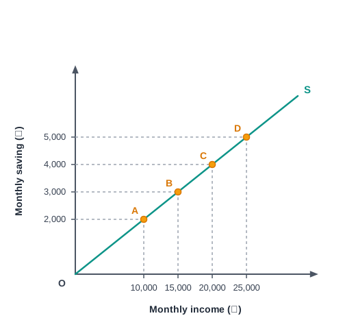
Fig. 22.1 – Income and saving of a household.
A graph shows at a glance what a schedule shows only after the columns have been compared. The upward slope of the line states the direction of the relationship, and the fact that the plotted points fall on a single straight line states that the rate of increase is unchanging.
Each form has its limits. A schedule reports only the levels actually listed, so Table 22.1 says nothing about saving at an income of ₹18,000. A graph covers the intermediate levels but has to be measured off by eye, and must be redrawn whenever the figures change.
22.1.3 The Mathematical Equation as a Third Way
The relationship in Table 22.1 can also be written as a single statement in symbols. Saving in that household is always one-fifth of income, and this is expressed by an equation which gives the value of saving for any value of income.
\[S = 0.2Y\]
Here \(S\) is monthly saving in ₹ and \(Y\) is monthly income in ₹. The equation is read as the instruction to multiply any level of income by 0.2 to obtain the corresponding level of saving.
The equation can be checked against the schedule. At an income of ₹15,000, it gives a saving of \(0.2 \times 15{,}000 = ₹3{,}000\), which is the figure Table 22.1 records. The two agree because they are the same relationship in different dress.
Its advantage is reach and precision. At an income of ₹18,000, a level the schedule does not list, the equation gives a saving of ₹3,600 exactly, without any measuring off a graph. It also states the rate of the relationship openly: the figure 0.2 in the equation is the amount by which saving rises for every one rupee rise in income.
The schedule, the graph and the equation are therefore three presentations of one relationship, and the choice between them is a matter of convenience. The rest of the chapter works mainly with the third, because it is the form in which a relationship can be stated exactly and its rate read off directly.
22.2 Functions
Section 22.1 ended with a relationship written as an equation. Before more can be done with equations of that kind, the idea behind them has to be named. When one variable depends on another in a definite way, so that fixing the value of the second fixes the value of the first, economists say that the first is a function of the second.
The word carries a precise meaning, and much of the notation used in the rest of the syllabus rests on it. This section explains what a function is, which of the two variables in a function does the depending, where functions are met with in economics, and what is added when the exact nature of a function is specified.
22.2.1 Meaning of a Function
A function is a relationship in which the value taken by one variable is determined by the value taken by another. Saying that saving is a function of income means that once the level of income is known, the level of saving is settled.
The relationship is written using the letter \(f\), which stands for the phrase ‘is a function of’.
\[S = f(Y)\]
Here \(S\) is saving and \(Y\) is income, and the statement is read as ‘saving is a function of income’. The letter \(f\) is not a quantity and is not multiplied by anything; it is only a way of writing that a definite rule connects the two variables.
A function can be pictured as a rule that receives a value and returns a value, as in Fig. 22.2.
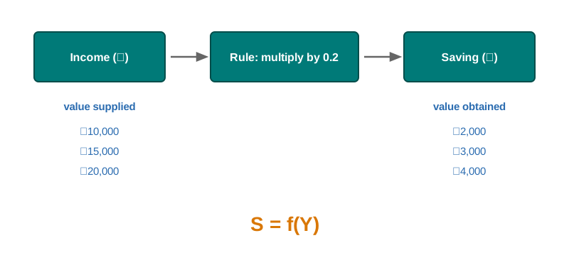
Fig. 22.2 – A function as a rule linking two variables.
The essential point is that the rule gives one and only one value in return. If a level of income of ₹15,000 could be accompanied by a saving of either ₹3,000 or ₹4,000, there would be no function, because knowing income would not settle saving.
22.2.2 Dependent and Independent Variables
The two variables in a function do not stand on the same footing. The variable whose value is determined is the dependent variable, and the variable whose value determines it is the independent variable. In \(S = f(Y)\), saving is dependent and income independent, because saving is being explained by income and not the other way round.
Which variable is treated as independent is decided by the economic reasoning, not by the algebra. Income is taken as independent in the saving function because a household must first earn before it can decide how much to set aside.
A function usually singles out one determinant and holds the others still. Quantity demanded depends on the price of the commodity, but also on income, on the prices of related goods and on tastes. Writing \(Q_d = f(P)\) isolates price and assumes the rest unchanged, an assumption stated as ceteris paribus, meaning ‘other things remaining equal’.
22.2.3 Functions Met With in Economics
Most of the relationships taught in economics are functions, and each is named after its dependent variable.
- Demand function — quantity demanded of a commodity as a function of its price, written \(Q_d = f(P)\), other determinants remaining unchanged.
- Supply function — quantity supplied of a commodity as a function of its price, written \(Q_s = f(P)\).
- Production function — output as a function of the quantity of a factor employed, written \(Q = f(L)\), where \(L\) is the number of workers.
- Cost function — total cost of production as a function of the level of output, written \(TC = f(Q)\).
- Saving function — saving of a household as a function of its income, written \(S = f(Y)\).
In each case the function states only that the dependent variable is governed by the independent one. It does not yet say in which direction the two move, or by how much the one changes when the other changes by a unit.
22.2.4 Meaning of a Functional Form
The exact rule connecting the two variables is called the functional form. Writing \(Q_d = f(P)\) states that a relationship exists; specifying the functional form states what the relationship is.
\[Q_d = 50 - 2P\]
Here \(Q_d\) is quantity demanded in units and \(P\) is price in ₹. The functional form says that 2 units of the commodity are given up for every one rupee rise in price, starting from 50 units at a price of zero. Table 22.2 sets out the values it yields.
Only with the functional form supplied can a schedule of this kind be drawn up or a graph plotted. The general statement \(Q_d = f(P)\) would have been consistent with countless different schedules; the form \(Q_d = 50 - 2P\) picks out one of them.
Functional forms differ in the pattern they impose. In the one above, quantity falls by the same 2 units for every rupee, whatever the price already is. In others the change is larger at some levels than at others. That distinction is taken up in the next section.
22.3 Linear and Non-Linear Functions
The last section ended with a functional form in which quantity demanded fell by the same 2 units for every one rupee rise in price, whatever the price already stood at. Relationships of that kind are the simplest to work with, because their rate of change never alters.
Not every economic relationship behaves so obligingly. In many of them the change in the dependent variable is large at first and smaller later, or the other way round. Functions are therefore divided into two classes according to whether the rate of change is constant, and the division decides the shape their graphs take.
22.3.1 Meaning of a Linear Function
A linear function is one in which a given change in the independent variable always produces the same change in the dependent variable, no matter where on the relationship the change occurs.
Table 22.2 in the last section illustrates this. Price rises in steps of ₹5, and quantity demanded falls by 10 units at every step — from 40 to 30, from 30 to 20 and from 20 to 10. The size of the fall does not depend on whether price is low or high.
The same steadiness appeared in Table 22.1, where every rise of ₹5,000 in income was accompanied by a rise of ₹1,000 in saving. Both relationships are linear, although one moves upward and the other downward.
22.3.2 The Graph of a Linear Function
When the pairs generated by a linear function are plotted and joined, the points lie on a straight line. Fig. 22.3 plots the four pairs of Table 22.2.
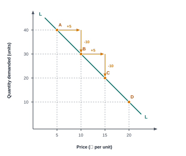
Fig. 22.3 – Graph of the linear function Qd = 50 - 2P.
The straightness of the line is not a drawing convention but a consequence of the arithmetic. Equal steps along the horizontal axis are matched by equal steps in the vertical direction, and a set of points spaced in that way can only lie on a straight line.
22.3.3 Meaning of a Non-Linear Function
A non-linear function is one in which equal changes in the independent variable produce changes of differing size in the dependent variable. Its graph is not a straight line but a curve.
Table 22.3 records the output of a small workshop as more workers are put on the same set of machines.
Each additional worker raises output, so the relationship is a rising one, but the addition made falls steadily from 16 units to 4. The independent variable moves in equal steps of one worker while the dependent variable does not, and the relationship is therefore non-linear. Fig. 22.4 shows the shape this produces.
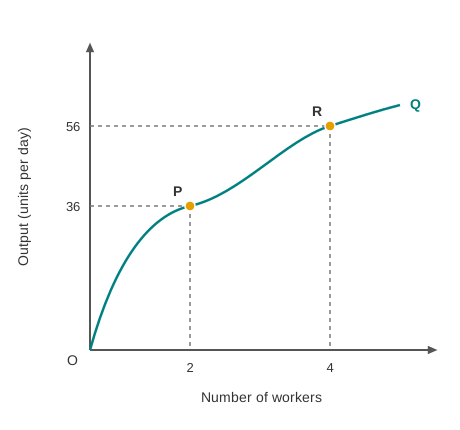
Fig. 22.4 – Graph of a non-linear function.
22.3.4 Difference Between Linear and Non-Linear Functions
The two classes are best held apart by asking what happens to the size of the change as the relationship is moved along. The main points of difference are set out below.
The syllabus takes the linear case further, because a straight line can be described completely by two numbers. What those numbers are, and how a straight line is written as an equation, is the subject of the next section.
22.4 The Equation of a Straight Line
A linear function has the convenient property that everything about it can be captured in two numbers: the value the dependent variable takes when the independent variable is zero, and the amount by which it changes for every unit of the independent variable. Fix those two numbers and the line is settled — no other straight line will pass through the same points.
The equation of a straight line is simply a way of writing those two numbers down in a single statement. This section gives the general form of that equation, explains what each of the two numbers stands for, and shows how a line is drawn once the equation is known.
22.4.1 The General Form of the Equation
Every straight line can be written in one standard form. It states the value of the dependent variable as a starting amount plus a fixed amount for each unit of the independent variable.
\[y = a + bx\]
Here \(y\) is the dependent variable, \(x\) the independent variable, \(a\) the value of \(y\) when \(x\) is zero, and \(b\) the amount by which \(y\) changes when \(x\) rises by one unit. Both \(a\) and \(b\) are constants, fixed for a given line, while \(x\) and \(y\) vary. The units of \(a\) are those of \(y\), and \(b\) is measured in units of \(y\) per unit of \(x\).
The letters carry no meaning of their own and are replaced by whatever the variables happen to be. The relationship met in Section 22.1 was \(S = 0.2Y\), with \(S\) in place of \(y\) and \(Y\) in place of \(x\); the demand relationship of Section 22.2 was \(Q_d = 50 - 2P\). Both fit the same general form.
22.4.2 The Intercept
The constant \(a\) is called the intercept. It is the value of the dependent variable when the independent variable is zero, and on a graph it is the point at which the line cuts the vertical axis.
Consider a tiffin service that pays a rent of ₹4,000 a month for its kitchen whether or not a single meal is cooked, and spends a further ₹50 on ingredients for each tiffin prepared. Its total monthly cost is
\[TC = 4{,}000 + 50Q\]
where \(TC\) is total cost in ₹ for the month and \(Q\) is the number of tiffins prepared. The intercept is ₹4,000, the cost the service must bear at an output of zero, and it fixes the height at which the line begins. Fig. 22.5 shows the position.
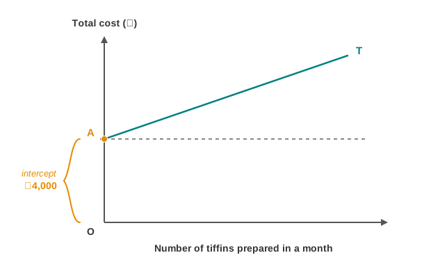
Fig. 22.5 – The intercept of a straight line.
The intercept is what the relationship contributes independently of the independent variable. In the tiffin service it is the cost that does not vary with the number of meals; in a bill it is the fixed charge; in a fare it is the amount payable before any distance is covered.
22.4.3 The Slope Parameter
The constant \(b\) is the slope parameter. It states the amount by which the dependent variable changes for every one-unit change in the independent variable, and it is what makes one straight line steeper than another.
In the tiffin service, \(b\) is 50, meaning that every additional tiffin adds ₹50 to total cost. In the saving relationship \(S = 0.2Y\), \(b\) is 0.2, so every additional rupee of income adds 20 paise to saving. In \(Q_d = 50 - 2P\), \(b\) is \(-2\), and quantity demanded falls by 2 units for every one rupee rise in price.
The sign of \(b\) carries the direction of the relationship and its size carries the steepness. A positive \(b\) gives a line rising from left to right, a negative \(b\) a line falling from left to right, and the larger the figure, the more sharply the line climbs or descends. How this parameter is measured off a graph is taken up in Section 22.6.
22.4.4 Drawing a Straight Line From Its Equation
Since two points determine a straight line, a line can be plotted from its equation without working out every value. The procedure has three steps.
- Choose two convenient values of the independent variable — zero is usually one of them, because it gives the intercept directly.
- Substitute each into the equation and work out the corresponding value of the dependent variable.
- Plot the two pairs on the graph and join them with a straight line, extending it as far as the relationship holds.
Applying this to \(TC = 4{,}000 + 50Q\), an output of zero gives a total cost of ₹4,000, and an output of 100 tiffins gives \(4{,}000 + 50 \times 100 = ₹9{,}000\). A third pair is worth working out as a check: at 60 tiffins the cost is \(4{,}000 + 50 \times 60 = ₹7{,}000\). The three pairs are set out in Table 22.4.
The three plotted points lie on one straight line, as shown in Fig. 22.6. Had any of them fallen off it, the arithmetic would have been at fault, since a linear equation cannot generate a point away from its own line.
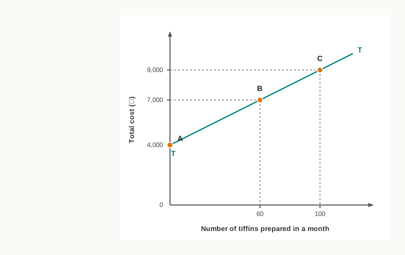
Fig. 22.6 – Drawing the line TC = 4,000 + 50Q.
22.4.5 Lines Passing Through the Origin
A line whose intercept is zero begins at the origin, and its equation loses the constant term altogether.
\[y = bx\]
Such a relationship says that the dependent variable is a fixed multiple of the independent variable, and that when one is zero so is the other. The saving relationship \(S = 0.2Y\) is of this kind: a household with no income saves nothing, and saving is always one-fifth of whatever is earned. Fig. 22.7 sets the two cases side by side.
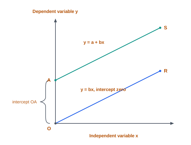
Fig. 22.7 – A line through the origin and a line with an intercept.
The two lines in the figure are parallel because they share the same slope parameter. They differ only in where they begin, which is the work the intercept does. Total cost that includes a fixed charge starts above the origin; total cost that is purely proportional to output starts at it.
22.5 The Direction of a Relationship
Two variables that are related must move either together or against each other. Either an increase in the one is accompanied by an increase in the other, or an increase in the one is accompanied by a decrease. There is no third possibility for a relationship in which the rate of change is constant.
This is the first question to settle about any relationship, and it is settled by the sign of the slope parameter \(b\) in \(y = a + bx\). A positive \(b\) means the variables move in the same direction, a negative \(b\) that they move in opposite directions. The section takes the two cases in turn.
22.5.1 Positively Related Variables
Two variables are positively related, or directly related, when a rise in the one is accompanied by a rise in the other and a fall by a fall.
Price and quantity supplied behave in this way. A higher price makes it worth a producer’s while to bring more of the commodity to market, and Table 22.5 sets out a schedule of that kind.
The equation of this relationship is \(Q_s = 20P\), where \(Q_s\) is quantity supplied in units and \(P\) is price in ₹ per unit. The slope parameter is 20 and carries no minus sign, and the intercept is zero because nothing is offered at a price of nothing. Plotted, the pairs give the rising line of Fig. 22.8.
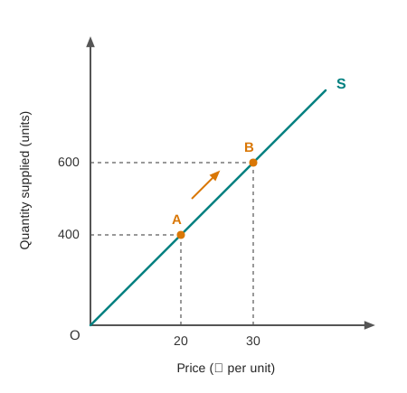
Fig. 22.8 – A positive relationship.
The examples of positive relationship met with earlier in the chapter run on the same lines. Saving rises as income rises, and output rises as more workers are employed, though only the first of these does so at a constant rate.
22.5.2 Negatively Related Variables
Two variables are negatively related, or inversely related, when a rise in the one is accompanied by a fall in the other.
The relationship \(Q_d = 50 - 2P\), introduced in Section 22.2, is of this kind. The minus sign before the 2 is not a slip in the arithmetic but the statement of direction: it says that quantity demanded falls as price rises. Written in the general form, a negative relationship reads
\[y = a - bx\]
where \(b\) is now the amount by which \(y\) falls for every one-unit rise in \(x\). Fig. 22.9 shows the line such a relationship produces.
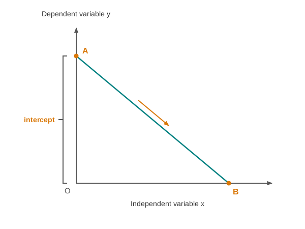
Fig. 22.9 – A negative relationship.
The line of a negative relationship must eventually meet the horizontal axis, because the dependent variable is falling by a fixed amount at every step and will in time be reduced to zero. In \(Q_d = 50 - 2P\) that happens at a price of ₹25, at which the quantity demanded works out to nil.
Direction, then, is the first thing an equation or a graph tells us, but it is not the whole of what a line says. Two lines may both rise, and yet one rise far more sharply than the other. Measuring that difference is the work of the slope.
22.6 The Slope of a Straight Line
Direction tells us whether a line rises or falls; it says nothing about how sharply. Two total cost lines may both rise with output, but the one belonging to a producer whose materials are dearer will climb faster. The measure of that steepness is the slope, and it is the single most useful number a straight line yields.
The slope answers a question economics asks constantly: when the independent variable changes by one unit, by how much does the dependent variable change? That is what an extra worker adds to output, what an extra rupee of income adds to saving, and what an extra unit of output adds to cost. This section defines the slope, shows how it is measured, and takes the special cases where it is zero or cannot be found at all.
22.6.1 Meaning of Slope
The slope of a straight line is the change in the variable measured on the vertical axis brought about by a one-unit change in the variable measured on the horizontal axis.
The slope and the parameter \(b\) of Section 22.4 are the same quantity. In \(y = a + bx\) the constant \(b\) was defined as the amount by which \(y\) changes when \(x\) rises by one unit, and that is exactly what the slope measures. Reading the slope off a graph and reading \(b\) off an equation are two routes to one number.
22.6.2 Measurement of Slope
To measure the slope, take any two points on the line, find how much the vertical variable has changed between them and how much the horizontal variable has changed, and divide the first by the second.
\[\text{Slope} = \dfrac{\Delta y}{\Delta x}\]
Here \(\Delta y\) is the change in the dependent variable between the two points and \(\Delta x\) the change in the independent variable, the symbol \(\Delta\) standing for ‘change in’. The slope is measured in units of \(y\) per unit of \(x\) — rupees per tiffin, units per worker, rupees per rupee of income — and it is read as the amount by which \(y\) alters when \(x\) alters by one.
Take the cost line \(TC = 4{,}000 + 50Q\) of Section 22.4 and the points B and C of Table 22.4. Between them, output rises from 60 tiffins to 100 and total cost from ₹7,000 to ₹9,000, so
\(\Delta y = 9{,}000 - 7{,}000 = ₹2{,}000\)
\(\Delta x = 100 - 60 = 40\) tiffins
\(\text{Slope} = \dfrac{2{,}000}{40} = 50\)
The slope is ₹50 per tiffin, which is the figure standing against \(Q\) in the equation. Fig. 22.10 shows how the two changes are read off the diagram.
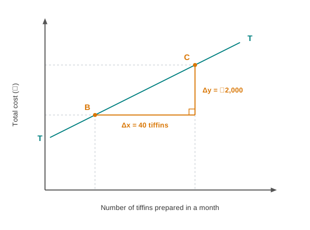
Fig. 22.10 – Measuring the slope of a straight line.
The same method applied to a falling line gives a negative answer. On \(Q_d = 50 - 2P\), price rising from ₹5 to ₹20 takes quantity demanded from 40 units to 10, so \(\Delta y = -30\) units, \(\Delta x = ₹15\), and the slope is \(-30 \div 15 = -2\) units per rupee.
22.6.3 Why the Slope of a Straight Line Is Constant
The slope of a straight line is the same wherever on the line it is measured. Had B and C in Fig. 22.10 been replaced by any other pair of points on TT, the ratio \(\Delta y / \Delta x\) would still have come to 50, because the line was drawn from an equation in which every additional tiffin adds the same ₹50.
This is the property that made the function linear in the first place. A constant rate of change produces a straight line, and a straight line in turn yields a constant slope; the two statements say the same thing from different ends. It also means a single triangle drawn anywhere on the line is enough to measure the slope of the whole of it.
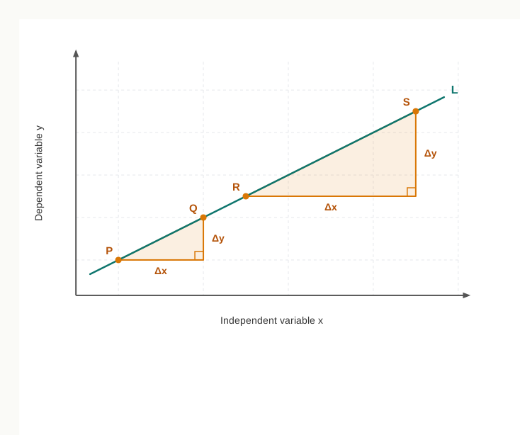
Fig. 22.11 – The slope is the same at every point on a straight line.
A curve behaves otherwise. On the workshop curve of Fig. 22.4 the same triangle drawn near the origin and drawn further to the right would give quite different ratios, because each additional worker there adds less than the last. Speaking of the slope of a curve therefore requires the point on it to be named, whereas a straight line has one slope and needs no such qualification.
22.6.4 Sign of the Slope
The sign of the slope repeats what Section 22.5 established about direction, now as a number rather than a description.
- Positive slope — the line rises from left to right and the two variables move in the same direction, as with price and quantity supplied.
- Negative slope — the line falls from left to right and the two variables move in opposite directions, as with price and quantity demanded.
The sign and the size are read separately and answer different questions. The sign says which way the relationship runs; the figure says how much the dependent variable responds. A slope of \(-2\) and a slope of \(-10\) both describe inverse relationships, but the second describes a far sharper response.
22.6.5 Slope of a Horizontal Line
A line drawn parallel to the horizontal axis has a slope of zero. The dependent variable takes the same value whatever the value of the independent variable, so \(\Delta y\) is nil at every step, and
\[\text{Slope} = \dfrac{0}{\Delta x} = 0\]
The equation of such a line is \(y = a\), the slope parameter having disappeared. A registration fee charged at the same amount whatever the quantity registered traces a horizontal line: the amount payable does not respond to quantity at all. A zero slope is the mark of no relationship between the two variables over the range drawn.
22.6.6 Slope of a Vertical Line
A line drawn parallel to the vertical axis presents the opposite case. Here the independent variable does not change at all, so \(\Delta x\) is zero, and the ratio \(\Delta y / \Delta x\) calls for a division by zero.
Division by zero yields no number, and the slope of a vertical line is therefore said to be undefined. Some books describe it instead as infinite, meaning that the line is as steep as a line can be drawn; the two descriptions point at the same fact, which is that no finite figure can be attached to it. The equation of such a line is \(x = k\), a constant, and the dependent variable is left free to take any value.
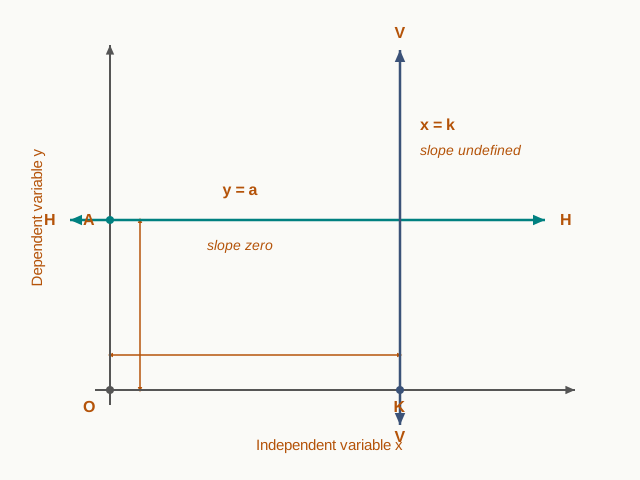
Fig. 22.12 – Horizontal and vertical lines.
The two cases close the account of the straight line. A line may rise, fall, run flat or stand upright, and in each case the slope — positive, negative, zero or undefined — states in one figure how the two variables of the relationship stand towards each other.
22.7 Summary
- A variable is a quantity that can take different values, while a constant is a quantity whose value does not change under the conditions being studied. Economics is concerned less with a single variable than with the settled way two variables move together, and every variable must be stated with its unit.
- A relationship between two variables can be presented in three ways, each carrying the same information.
- A schedule, which lists paired values but reports only the levels actually shown.
- A graph, which shows the direction and steadiness of the relationship at a glance but must be measured off by eye.
- An equation, which covers every level of the independent variable and states the rate of the relationship exactly.
- A function is a relationship in which the value of one variable is determined by the value of another, so that to each value of the second there corresponds a definite value of the first. It is written \(S = f(Y)\), read as ‘saving is a function of income’, where \(f\) stands for the rule connecting the two and is not a quantity to be multiplied.
- The variable whose value is determined is the dependent variable and the variable that determines it is the independent variable. Which is which is decided by the economic reasoning, and the remaining determinants are held constant by the assumption of ceteris paribus.
- Functions are met with throughout the subject — the demand function \(Q_d = f(P)\), the supply function \(Q_s = f(P)\), the production function \(Q = f(L)\), the cost function \(TC = f(Q)\) and the saving function \(S = f(Y)\). Each names the dependent variable first and the determinant in the bracket.
- Writing \(Q_d = f(P)\) states only that a relationship exists. The functional form, such as \(Q_d = 50 - 2P\), states what the relationship is, and only with the form supplied can a schedule be drawn up or a graph plotted.
- A linear function is one in which the dependent variable changes by a constant amount for every one-unit change in the independent variable, and its graph is a straight line. A non-linear function is one in which that change differs from one level to another, and its graph is a curve. The distinction turns on the size of the change, not its direction.
- Every straight line can be written in one standard form. \[y = a + bx\] Here \(y\) is the dependent variable, \(x\) the independent variable, \(a\) the intercept and \(b\) the slope parameter. Both \(a\) and \(b\) are constants for a given line, the units of \(a\) being those of \(y\) and \(b\) being measured in units of \(y\) per unit of \(x\).
- The intercept \(a\) is the value of the dependent variable when the independent variable is zero, and is the point at which the line cuts the vertical axis. It fixes the height at which the line begins. Where the intercept is zero the equation becomes \(y = bx\) and the line passes through the origin.
- The slope parameter \(b\) is the amount by which the dependent variable changes for every one-unit change in the independent variable. Changing \(a\) shifts the whole line up or down; changing \(b\) tilts it.
- A line is drawn from its equation by choosing two convenient values of the independent variable, working out the corresponding values of the dependent variable and joining the two points, taking a third pair as a check.
- Two variables are positively related when they move in the same direction, as price and quantity supplied do, and negatively related when they move in opposite directions, as price and quantity demanded do. The direction is read off the sign of \(b\), and a negative relationship does not mean that either variable takes a negative value.
- The slope of a straight line is the ratio of the change in the dependent variable to the change in the independent variable between two points on it. \[\text{Slope} = \dfrac{\Delta y}{\Delta x}\] Here \(\Delta y\) is the change in the dependent variable, \(\Delta x\) the change in the independent variable and \(\Delta\) stands for ‘change in’. The result is expressed in units of \(y\) per unit of \(x\), and is the same quantity as the parameter \(b\) in the equation of the line.
- The slope is measured by drawing a right-angled triangle against the line between any two points and dividing the vertical side by the horizontal side. The order of subtraction must be the same in both parts of the ratio, or the sign comes out reversed.
- The slope of a straight line is the same wherever it is measured, since a constant rate of change and a straight line are two statements of one fact. The slope of a curve differs from point to point, so the point must be named before it can be spoken of.
- The sign and the size of the slope answer different questions. A positive slope marks a rising line, a negative slope a falling one, and the larger the figure in size, the sharper the response of the dependent variable.
- Two limiting cases complete the account.
- A horizontal line has a slope of zero, since \(\Delta y\) is nil at every step. Its equation is \(y = a\), and the two variables do not respond to each other over the range drawn.
- A vertical line has an undefined slope, since \(\Delta x\) is zero and the ratio would call for a division by zero. Its equation is \(x = k\).
22.8 Points to Ponder
- A functional form such as \(Q_d = 50 - 2P\) can be used to work out the quantity demanded at any price whatever, including prices far outside the range from which the relationship was drawn up. How far beyond the observed levels should such an equation be trusted, and what would warn you that it had been pushed too far?
- Writing \(Q_d = f(P)\) isolates price and holds income, tastes and the prices of related goods constant. Every relationship a student meets in economics is stated under some such assumption. Does the convenience of studying one determinant at a time come at a cost, and if so, what is given up?
- The saving relationship of Section 22.1 passes through the origin, so a household with no income saves nothing. Is that a reasonable description of a real household, and what would the line look like if a household with no income had to draw down past savings instead?
- The workshop schedule of Section 22.3 shows output rising by smaller and smaller amounts as workers are added, while the cost line of Section 22.4 rises by a constant ₹50 for every tiffin. Which of the two patterns would you expect to be commoner in an economy, and why might a textbook nevertheless teach the straight line first?
- A slope of zero means the dependent variable does not respond at all to the independent one over the range drawn. Does a zero slope establish that the two variables are unrelated, or only that the relationship does not show up in the range that has been examined?
- The intercept of a demand relationship is the quantity that would be demanded at a price of zero — a level no market ever reaches. Is a number that describes a situation which cannot occur still worth having in the equation?
22.9 Objective Questions
- The slope of a line drawn parallel to the vertical axis is: [1]
- zero
- one
- undefined
- negative
- Assertion (A): The slope of a straight line is the same wherever on the line it is measured. [1] Reason (R): In a linear function the dependent variable changes by a constant amount for every one-unit change in the independent variable.
- Both A and R are true, and R is the correct explanation of A.
- Both A and R are true, but R is not the correct explanation of A.
- A is true but R is false.
- A is false but R is true.
- In the equation of a straight line \(y = a + bx\), the constant \(a\) is known as the ______ of the line. [1]
- State whether the following statement is true or false: A relationship with a negative slope is one in which both variables take negative values. [1]
- Match the lines in Column A with their properties in Column B: [1]
| Column A | Column B |
|---|---|
| a. A line drawn parallel to the horizontal axis | i. Intercept is zero |
| b. A line passing through the origin | ii. Slope is negative |
| c. A line falling from left to right | iii. Slope is zero |
22.10 Check Your Concepts
- Define a function. In the supply function \(Q_s = f(P)\), name the dependent and the independent variable. [2]
- Distinguish between a linear and a non-linear function on any three bases. [3]
- The total cost of a small unit is given by \(TC = 3{,}000 + 40Q\), where \(TC\) is total cost in ₹ for the month and \(Q\) is the number of units produced. State the intercept and the slope of this relationship, calculate the total cost of producing 50 units, and state in one sentence what the slope means here. [4]
- The monthly saving of a household at four levels of monthly income is given below.
| Monthly income (₹) | 12,000 | 16,000 | 20,000 | 24,000 |
|---|---|---|---|---|
| Monthly saving (₹) | 1,800 | 2,400 | 3,000 | 3,600 |
Show that the relationship is linear, calculate its slope, draw the line on a graph with income on the horizontal axis, and explain what the sign and the size of the slope tell you about the two variables. [6]
22.11 Case-Based Question
- Farida runs a photocopying shop in a market lane. She pays a rent of ₹3,500 a month for the shop whether or not a single page is copied, and spends ₹1 on paper and toner for every page she copies. She has begun writing her total monthly cost as an equation so that she can work out in advance what any level of business will cost her.
- Write the equation of Farida’s total monthly cost, stating clearly what each symbol represents, and give the value of the intercept. [2]
- Calculate her total cost in a month in which 6,000 pages are copied, and state what the slope of her cost line measures. [2]