Chapter 2: Demand and Law of Demand
Every buyer faces the same problem. Wants run ahead of income, so at the price being asked a household must decide how much of a good is worth buying and what it is willing to give up for it. Demand is the economist’s record of those decisions, and one of the two forces that settle price in a market. When the Government of India launched the UJALA scheme in 2015, bulk procurement brought the price of an LED bulb down sharply. Households that had bought one bulb to try began replacing the lamps in every room. The bulb had not changed. Its price had, and the quantity buyers were willing to take moved in the opposite direction. That inverse relationship is what the law of demand states and what the demand curve pictures, but price is only one of the influences on a buyer. This chapter explains what demand means and the forms it takes, sets out the factors that determine it, states and illustrates the law of demand and the reasons behind it, notes the situations in which the law does not hold, and distinguishes a movement along the demand curve from a shift of the whole curve.
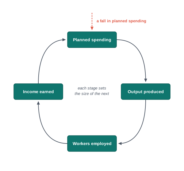
Fig. 2.0 – Determinants of demand and their effects.
2.1 Meaning of Demand
Economic theory begins from a plain question: why does a good command a price at all, and why is one good dearer than another? The answer has two halves. A good is paid for only if it is useful to somebody, and it can be charged for only if it is scarce in relation to what people would like to have of it. Usefulness alone will not do, and scarcity alone will not do. A price arises where the two meet.
Usefulness expresses itself in the market as demand by buyers, and scarcity expresses itself as supply by sellers. Between them these two forces settle the price and the quantity traded of everything sold in a free market, which is why demand and supply are the two working tools of price theory. This chapter takes up the first of the pair.
2.1.1 Economic Goods and Free Goods
Not everything useful has a price. Air is essential to life, yet nobody pays for the air breathed on a morning walk. It is useful in the highest degree, but it is not scarce, since there is more of it at hand than anyone could want. Free goods are the gifts of nature available in unlimited quantity at the place and time concerned, and because they are not scarce they command no price.
Economic goods are scarce in relation to the quantity people would like to have. Cloth, foodgrains, cars and cement are all useful, and every one of them is limited, so each has to be produced with resources that could have been put to some other use. That is why economic goods command a price, and why they, rather than free goods, form the subject matter of economics.
The line between the two is drawn by scarcity, and scarcity can change. Water drawn from a village well is a free good. The same water, cleaned and carried to a city where clean water is short, is an economic good with a price attached to it. A good is free or economic according to its supply relative to want, not according to its nature.
The main points of difference are set out below.
2.1.2 Essential Features of Demand
In ordinary speech, to demand a good is much the same as to want it. In economics the word is far narrower. A wish is a state of mind and costs the person nothing; what the market records is the quantity a buyer is actually prepared to take off the shelf at a stated price. That quantity is what economists mean by demand.
Three conditions are packed into this definition, and an answer that leaves any of them out is incomplete.
- Demand is effective desire — a wish for a good becomes demand only when it is backed by the money to pay for it and by the willingness to part with that money. A student may long for a motorcycle, but that longing enters the market only when he has the price of one and is prepared to spend it. Desire without purchasing power, and purchasing power without willingness, both stay outside the demand for the good.
- Demand is always at a price — a quantity demanded means nothing until the price at which it would be bought is stated. The same household may buy four shirts when each costs ₹500 and only one when the price is ₹800, so the demand for shirts is not a single number but a whole list of quantities, one against each possible price.
- Demand is always for a period of time — demand is a flow, that is, a variable measured per unit of time. Two hundred cars a day, 1,400 cars a week and 73,000 cars a year describe one and the same flow, while the bare figure 200 describes nothing. Demand refers to a continuing stream of purchases and not to a single act of buying.
To say that the demand for cars is 200 is therefore an unfinished statement. Two hundred at what price, and over what period? Once the price and the period are attached, the figure means something, and it can be set beside the quantity that would be bought if the price were higher or lower. Comparing those quantities is the whole business of the law of demand, and the sections that follow build up to it.
2.2 Types of Demand
The same quantity of a good can be looked at from several angles. We may ask how many buyers stand behind it, whether it is a quantity that was planned or one that was actually bought, and whether the good is wanted on its own or alongside something else. Each question gives a different classification of demand, and five of them are used repeatedly in this course: individual and market demand, ex ante and ex post demand, joint demand, derived demand and composite demand.
These are not five rival meanings of the word. They are five ways of describing the same thing, and which one is needed depends on the question being asked.
2.2.1 Individual Demand and Market Demand
Demand may be counted for one buyer or for the whole market. The buying unit in economics is the household rather than the person, since a family usually decides its purchases together and pays for them out of a common income. Individual demand and household demand therefore mean the same thing. The quantity of milk a family takes each day at the price it is charged is an individual demand.
A market, however, is made up of many such households. What a seller faces is not the demand of any one of them but the demand of all of them together, and it is this total that settles the price.
Market demand is obtained by taking one price at a time and adding up the quantities that every household in the market would buy at that price. The addition is repeated for each price, which gives a list of market quantities, one against each price. How this addition is carried out on a diagram is shown in section 2.4.4.
Because market demand depends on how many households there are, it can change even when no single household has altered its own buying. If new families move into a town, the market demand for milk there rises although every existing family buys exactly as before. The two are set apart on the following points.
2.2.2 Ex Ante and Ex Post Demand
A household plans its purchases before it reaches the market, and what it carry home need not match what it set out to buy. Economics keeps the two apart. Planned demand is called ex ante demand and realised demand is called ex post demand.
The two figures part company whenever the good is not available in the quantity intended. A family that plans to buy five kilograms of a foodgrain in a week, and finds only three kilograms in the shops, has an ex ante demand of five kilograms and an ex post demand of three. The gap between them is a signal of shortage. The same distinction returns in the theory of income and employment, where planned spending by the economy as a whole is set against the spending actually realised.
2.2.3 Joint, Derived and Composite Demand
Goods are rarely wanted in isolation. Some are useful only in the company of another good, some are wanted only because something else is wanted, and some serve several purposes at once. Three further types of demand record these relations.
- Joint demand — the demand for two or more goods that are used together and are therefore wanted together, such as bread and butter, or a cricket bat and a ball. Goods in joint demand move together: whatever raises the quantity bought of one raises the quantity bought of the other, and a rise in the price of one reduces the purchase of both.
- Derived demand — the demand for a good that arises out of the demand for some other good. Nobody wants cement or bricks for their own sake; they are wanted because houses and roads are being built, so their demand is derived from the demand for buildings. The demand for factors of production is always derived in this way, since a mill hires weavers only because there is a demand for the cloth they make.
- Composite demand — the demand for a good that has several distinct uses, the total being the sum of the amounts wanted for each of them. Electricity is wanted for lighting homes, for pumping water on farms and for running machines in factories. Because these uses compete for the same supply, more of it drawn by one use leaves less for the others, and a change in its price alters the quantity taken by every use at once.
These labels describe one quantity seen from different sides. The rest of the chapter works with individual and market demand, for it is there that the influence of price, which the law of demand sets out, can be traced most clearly.
2.3 Determinants of Demand
A buyer standing in a shop weighs several things at once. The price on the label matters, but so does the money in hand, the price of the substitute on the next shelf, what the neighbours have bought and what prices are expected next month. The factors that influence a household’s decision to buy a commodity are called the determinants of demand.
Economics separates them for a reason. Only one of them, the own price of the good, is allowed to vary in the law of demand; every other determinant is held still while that law is stated. Before the law can be stated properly, therefore, the full list has to be set out.
2.3.1 Determinants of Individual Demand
Seven factors decide how much of a commodity a single household will buy.
- Price of the commodity — the own price of the good is the chief determinant, and normally the quantity bought moves in the opposite direction to it. The different quantities a household would buy at different prices, with everything else unchanged, are together called its price demand, and the law of demand in section 2.4 is a statement about them.
- Income of the consumer — income fixes purchasing power, so for most goods a richer household buys more. The relation between the level of income and the quantity bought, price unchanged, is called income demand, and it does not run in the same direction for every kind of good.
- Prices of related goods — the demand for a good depends on the prices of goods that can replace it or that are used along with it. The relation between the demand for one good and the price of another is called cross demand.
- Tastes and preferences — custom, fashion, advertisement, climate of opinion and general style of living decide what a household wants in the first place. A change in taste in favour of a good raises its demand at every price, and a change against it lowers demand at every price.
- Consumers’ expectations — what buyers expect about future prices and their own future income affects what they buy today, because goods can be stored and purchases can be postponed. An expected rise in price brings buying forward; an expected fall pushes it back.
- Consumer credit facilities — a household that can borrow, or buy on instalments, can purchase goods its current income alone would not stretch to. Credit chiefly affects the demand for costly durable goods such as vehicles and household appliances.
- Demonstration effect — households tend to copy the consumption of friends, neighbours and relations, so a good bought by others is wanted for that reason alone. This effect works strongly on goods that are seen in use.
Income Demand And The Three Kinds Of Goods
Income raises purchasing power, but the goods a household turns to as it grows richer are not the goods it turns away from. On the response of demand to income, goods fall into three groups.
Clothing, packaged foods, refrigerators, televisions and vehicles are normal goods for most households. As income rises the family can afford more of them, so income and quantity demanded move in the same direction.
A good is inferior only in this technical sense. At low incomes a household buys more of it as income rises, exactly as with a normal good; but once income passes a certain level the better substitute comes within reach and purchases of the inferior good begin to fall. The third group, inexpensive necessities such as salt or matchboxes, behaves differently again: demand rises with income up to a point and then stays flat, since there is a natural limit to how much of them a family can use. The three responses are drawn together in Fig. 2.1.
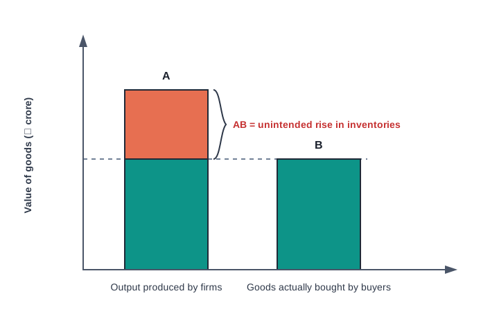
Fig. 2.1 – Income demand for normal, inferior, and inexpensive necessity goods.
Cross Demand: Substitutes And Complements
Goods are related in two ways that matter for demand, and the two work in opposite directions.
Substitute goods satisfy the same want and can be used in place of one another, as tea and coffee can. If the price of coffee rises while the price of tea stays where it was, coffee has become dearer relative to tea, and buyers move across. The demand for tea therefore rises although nothing has happened to its own price. This direct relation between the demand for a good and the price of its substitute is drawn in Fig. 2.2.
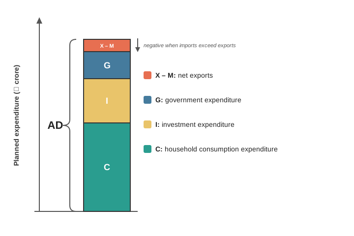
Fig. 2.2 – Cross demand for a substitute good.
Complementary goods are used together, so that one is of little use without the other, as a car is without petrol. If the price of petrol rises, running a car becomes costlier, and fewer cars are bought even though the price of cars has not moved. This inverse relation is drawn in Fig. 2.3.
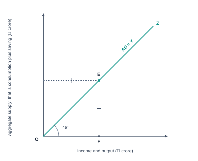
Fig. 2.3 – Cross demand for a complementary good.
The main points of difference between the two kinds of related goods are set out below.
2.3.2 Additional Determinants of Market Demand
Everything said so far applies to the market as well, since market demand is only the sum of household demands. Four further factors work on that sum rather than on any one household.
- Size and composition of population — the number of people in a market fixes the number of possible buyers, so a growing population raises market demand for most goods. Composition matters as much as size, because a market with many young people demands goods that a market of elderly people does not.
- Distribution of income — the same national income spread evenly and spread unevenly produce different demands. Where income is concentrated in few hands the market demand for luxuries is larger, and where it is evenly spread the demand for necessities is larger.
- Climatic conditions — demand for coolers, fans and cold drinks rises in the hot months, and demand for woollens and hot drinks rises in the cold ones. In a country as varied as India this produces sharply different regional demands for the same good.
- Government policy — a tax on a good raises the price buyers pay and so cuts the quantity demanded, while a cut in tax rates or in income tax leaves households with more to spend. Public expenditure works in the same way by putting income into people’s hands.
2.3.3 The Demand Function
The eleven determinants can be stated together in one line. A demand function states the relationship between the demand for a commodity and the factors that determine it: it names the cause and effect relation without saying how strong any one influence is.
\[D_n = f(P_n,\ P_1 \dots P_{n-1},\ Y,\ T,\ E,\ H,\ \bar{Y},\ G)\]
Here \(D_n\) is the quantity demanded of commodity \(n\), measured in units per period of time; \(f\) stands for the functional relation; \(P_n\) is the own price of the commodity in ₹; \(P_1 \dots P_{n-1}\) are the prices of all other commodities; \(Y\) is the income of the consumer in ₹ per period; \(T\) stands for tastes and preferences; \(E\) for expectations; \(H\) for the size and composition of population; \(\bar{Y}\) for the distribution of income; and \(G\) for government policy. The equation is read from left to right: the quantity demanded, the dependent variable, depends on all the variables listed on the right, which are the independent variables.
Nothing in the function is measured by writing it down. Its use is that it makes the assumption behind the law of demand visible. If every variable on the right except the own price is held constant, the function shortens to \(D_n = f(P_n)\), and demand becomes a relation between one quantity and one price. That shortened function is what a demand schedule tabulates and a demand curve draws.
A demand function of this narrow kind is often written in the straight line form \(Q_d = a - bP\), where \(a\) is the quantity that would be demanded if the good were free and \(b\) measures how much the quantity falls for each rupee added to the price. The minus sign is the law of demand written into the equation.
2.4 Law of Demand
Of all the factors that settle how much a household buys, only one is under the seller’s hand and only one changes from hour to hour in a market: the price of the good itself. Price theory therefore isolates that factor. It holds every other determinant still and asks a single question — if nothing else about the buyer or the market alters, what happens to the quantity taken when the price moves?
The answer is the law of demand. It is the best known statement in economic theory, and the demand schedule and the demand curve are the two ways of setting it out.
2.4.1 Statement of the Law
Buyers take more of a good when it is cheap and less of it when it is dear. Put formally, the price of a commodity and the quantity demanded of it move in opposite directions, provided the other determinants of demand do not change.
Two features of the statement deserve attention. First, the relationship it asserts is inverse, so price and quantity always move in opposite directions along it. Second, the law states a direction and not a magnitude. It says that a fall in price raises the quantity demanded; it does not say by how much. Measuring the size of the response is the work of elasticity of demand, taken up in the next chapter.
2.4.2 Assumptions of the Law
The law holds the other determinants of demand constant, which is what ceteris paribus means. Those determinants have not disappeared; they have been set aside so that the effect of price alone can be seen. Each assumption below therefore names one thing that must not move while the law is applied.
- Income of the consumer does not change — if income rose at the same time as the price, the quantity bought would be responding to two causes at once and the effect of price could not be separated out.
- Tastes and preferences do not change — a good that has just come into fashion may sell more at a higher price, which would hide the working of the law rather than disprove it.
- Prices of related goods remain unchanged — if the price of coffee moved along with the price of tea, the change in the quantity of tea bought would be partly a cross effect and not the effect of tea’s own price.
- The commodity is a normal commodity — the law is stated for ordinary goods, not for Giffen goods or for articles bought as a mark of status, which are taken up in Section 2.6.
- The size and age composition of the population do not change — for market demand, more buyers would raise the quantity taken at every price and would be mistaken for a response to price.
- The distribution of income does not change — a redistribution alters the pattern of demand between necessities and luxuries even when total income and prices are exactly as before.
- No change in price is expected in the future — a buyer who expects a further fall will wait rather than buy, so the response to today’s price would be masked by the expectation.
2.4.3 Demand Schedule
The simplest way to display the law is to write the quantities against the prices in a table. Such a table is called a demand schedule, and like demand itself it comes in two forms, individual and market.
An individual demand schedule records the quantities one household would buy. Table 2.1 sets out such a schedule for apples at four prices.
The table is read one line at a time. At ₹100 a kilogram the household would buy 1 kg a week; if the price fell to ₹90 it would buy 2 kg, and at ₹70 it would take 6 kg. Nothing else about the household is supposed to change between one line and the next. The quantity rises at every step as the price falls, which is the law of demand in numbers.
A market demand schedule is obtained by adding, at each price, the quantities that every household in the market would buy. Suppose apples in a small market are bought by two households, A and B. Table 2.2 puts their schedules side by side and adds them.
At ₹100 the market takes 3 kg, being 1 kg bought by A and 2 kg by B; at ₹70 it takes 13 kg. The addition is done price by price and never across prices, and the same method serves however many households there are in the market. The market schedule shows the same inverse relation as the individual schedule, because it is built out of individual schedules that each show it.
2.4.4 Demand Curve and its Derivation
A schedule gives the relation as a set of pairs; a curve gives it as a picture. Plotting each price-quantity pair as a point and joining the points produces the demand curve.
The four pairs of Table 2.1 are plotted in Fig. 2.4, with price measured on the vertical axis and quantity on the horizontal axis. Point a stands for the first line of the schedule, 1 kg bought at ₹100, and the remaining points stand for the lines below it.
Fig. 2.4 – Individual demand curve for apples.
The curve slopes downward from left to right, which is the graphical form of the inverse relation. A single point on it reports one price-quantity pair; the curve as a whole reports the entire relation, and it is drawn on the assumption that everything except the price of apples stays where it was.
The market demand curve is derived from the individual demand curves by horizontal summation, that is, by adding the quantities of all buyers at each separate price. Fig. 2.5 carries out the addition of Table 2.2 in three panels.
Fig. 2.5 – Derivation of market demand by horizontal summation.
At the price of ₹100 the two households take 1 kg and 2 kg, and adding these gives point A on the market curve at 3 kg. At ₹80 they take 4 kg and 5 kg, giving point B at 9 kg. Joining such points yields DM, the market demand curve, which slopes downward for the plain reason that both the curves it is built from do.
Why the curve should slope downward at all is a separate question, and one the law itself does not answer. The next section sets out the reasons behind it.
2.5 Reasons for the Downward Slope of the Demand Curve
The law of demand describes what buyers do; it does not say why they do it. A curve that slopes downward from left to right is a statement of fact about behaviour, and the fact stands in need of an explanation. Why should a household that was content with 1 kg of a good at a high price want 6 kg of the same good once the price has fallen?
Five reasons are usually given. The first three explain the behaviour of a single buyer, and the last two explain why the market curve slopes even more clearly than any individual curve within it.
2.5.1 Law of Diminishing Marginal Utility
Goods are bought because they satisfy wants, and the want-satisfying power of a commodity is called utility. The utility added by one more unit of the commodity is its marginal utility. As a household consumes more of the same good in a given period, each successive unit meets a want less urgent than the one before it, so marginal utility falls.
A buyer parts with money for a unit only if that unit is worth at least what it costs, and stops buying where the two are just equal. The condition for consumer’s equilibrium in one commodity is therefore written as follows.
\[MU = P\]
Here \(MU\) is the marginal utility of the last unit bought, measured in money terms as the maximum the buyer would be willing to pay for that unit in rupees, and \(P\) is the price of the commodity in rupees per unit. The condition is read as a stopping rule: the household goes on buying until the worth of the last unit to it has come down to the price it must pay.
The consequence for the demand curve follows at once. Since marginal utility falls as quantity rises, a buyer already in equilibrium will take an additional unit only if the price comes down to the lower worth of that unit. More is bought only at a lower price, which is exactly what a downward sloping curve says. The law of diminishing marginal utility is examined in full in the chapter on utility analysis.
2.5.2 Income Effect
A change in price changes what a given income can buy, and that by itself alters the quantity demanded. Two senses of income must be kept apart here. Money income is income counted in rupees, and it is unaffected by the price of any good. Real income is the purchasing power of that money income, that is, the quantity of goods and services it will actually fetch, and a fall in any price raises it.
Suppose a household buys 5 litres of cooking oil a month at ₹160 a litre and so spends ₹800 on it. If the price falls to ₹140 a litre, the same 5 litres now cost ₹700. The household’s money income has not moved by a rupee, yet ₹100 has been released. Its real income has risen, and a part of that gain is ordinarily spent on the good whose price fell, so the quantity of oil taken rises.
2.5.3 Substitution Effect
A price never falls on its own; it falls relative to the prices of every other good. When the price of a commodity comes down and the prices of its substitutes stay where they were, the commodity becomes cheaper in comparison with them, and buyers who were using the substitutes move across to it.
If the price of coffee falls while tea remains as dear as before, coffee becomes the better bargain of the two. Buyers who maximise satisfaction from a limited income shift towards the cheaper good, so the quantity of coffee demanded rises for a reason that has nothing to do with what the household can now afford in total.
In a real purchase the two effects are not felt one after the other; both are set off by the same price change and work at the same moment. Their sum is what is actually observed, and that sum is called the price effect.
\[\text{Price effect} = \text{Income effect} + \text{Substitution effect}\]
Each of the three terms is a change in quantity demanded, measured in units per period of time. The equation is read as a division of a single observed change into its two sources: part of the extra quantity bought is due to the buyer being better off in real terms, and part to the good having become cheaper than its rivals.
2.5.4 Number of Consumers and Several Uses of a Commodity
The two reasons taken up here work on the market demand curve rather than on the demand curve of one household, since neither the number of buyers nor the range of uses can alter for a single household whose curve is being drawn.
The first is the entry of new buyers. At a very high price only well-off households can afford a commodity at all, and the quantity taken by the market is small. As the price falls, households of moderate means come within reach of it, and at still lower prices poorer households join them. Every one of these newcomers adds a quantity that was not in the market before, so the total quantity demanded rises for a reason quite separate from any change in what existing buyers do.
The second is the several uses a commodity can be put to. Where a good serves more than one purpose, the uses can be ranked by how urgent they are. At a high price the good is kept for the most important use alone; as the price falls it is drawn into the less important uses as well, and the quantity taken by the market rises with each use it becomes worth putting the good to.
Taken together the five reasons say the same thing from five directions: at a lower price the good is worth buying in larger quantity, worth buying by more people, and worth putting to more uses. That is why the curve slopes downward, and why the cases in which it does not are so few. Those cases are the subject of the next section.
2.6 Exceptions to the Law of Demand
The law of demand holds in the great majority of markets, but it is a statement about ordinary goods bought by ordinary buyers under stated assumptions, and there are situations in which it fails. In those situations more of a commodity is bought at a higher price and less of it at a lower price, so the inverse relation between price and quantity no longer holds. These situations are called the exceptions to the law of demand.
When the law fails, the demand curve does not slope downward. It slopes upward from left to right, as in Fig. 2.6, and price and quantity rise and fall together.
Fig. 2.6 – Positively sloping demand curve.
2.6.1 Giffen Goods
The first and best known exception was pointed out by Sir Robert Giffen, a nineteenth century economist, and the goods concerned carry his name. Giffen goods are inferior goods of a particular kind: goods on which a poor household spends a large share of its income, and which have superior substitutes within reach once the household is a little better off.
The explanation turns on the difference between money income and real income. When the price of such a good falls, the household’s money income is unchanged but its real income rises sharply, because the good took up so much of its spending in the first place. With that gain the household buys some of the superior food it could not afford before. Since there is a limit to how much grain any family can eat, the extra purchase of the superior good must come at the cost of the inferior one, and the quantity of the cheap good bought actually falls when its price falls.
The relation between the two ideas is worth stating plainly, since the terms are often confused in answers.
2.6.2 Articles of Snob Appeal
Some goods are bought less for what they do than for what owning them says about the owner. Diamonds, rare paintings and costly antiques serve as marks of wealth and standing, and a high price is part of what makes them serve that purpose. Thorstein Veblen called such buying conspicuous consumption, and the behaviour is known after him as the Veblen effect.
If the price of a diamond falls far enough for many households to own one, it stops being a mark of distinction and the wealthy buyer’s reason for owning it disappears. The demand for such goods therefore rises with the price and falls when the price falls, which is the opposite of the law. Goods of this kind remain exclusive only so long as their prices stay high.
2.6.3 Other Exceptions
Four further situations are commonly listed.
- Expectations about future prices — when the price of a commodity is rising and buyers expect it to rise further, they buy more at the higher price rather than wait, and stock what they can. The same works in reverse: if a large fall is expected, purchases are postponed even after the price has begun to come down.
- Emergencies — during a war, a famine or a threatened shortage, households buy and hoard goods at prices they would normally refuse to pay, because being without the good is the greater risk. In a depression the opposite happens and buyers hold back even at low prices.
- Quality judged by price — where buyers cannot judge quality for themselves, they take the price as the sign of it. Of two nearly identical products, the dearer one may sell more simply because buyers read the higher price as proof of the better article.
- Change in fashion — a commodity that has gone out of fashion finds few buyers however far its price is cut. A style of kurta that no one is wearing this season will not sell in quantity at half price, because the fall in price does not restore the want.
That distinction applies to more than one item on the list. Expectations about future prices and changes in fashion are already covered by the assumptions of the law, which require expectations and tastes to stay constant. When these situations arise, the law is not being contradicted; it is simply not being applied under the conditions it was stated for. Giffen goods and articles of snob appeal are the harder cases, because in them the quantity moves the wrong way while the assumptions hold.
None of this unsettles the law. The exceptions cover a small number of goods and a small number of occasions, and for almost everything bought in an ordinary market the quantity taken still rises when the price falls. What remains to be sorted out is a different matter altogether: the difference between a change in quantity demanded caused by price, and a change in demand caused by everything else.
2.7 Movement Along and Shift of the Demand Curve
‘Demand for cars has gone up’ can mean two quite different things. It can mean that cars have become cheaper and buyers are taking more of them, or it can mean that incomes have risen and buyers are taking more cars than before at the very same price. In ordinary speech the two are not separated. In economics they must be, because they work through different causes and are drawn differently.
The distinction follows straight from the way a demand curve is constructed. A curve is drawn for one set of values of income, tastes, related prices and expectations; only the good’s own price is allowed to vary along it. So a change in the own price moves the buyer to another point on the same curve, while a change in anything else makes the old curve wrong and a new one has to be drawn.
2.7.1 Change in Quantity Demanded
When the own price of a commodity changes and nothing else does, the buyer moves along the existing demand curve. This is called a change in quantity demanded.
A change in quantity demanded takes two forms. An expansion of demand, also called a rise in quantity demanded, is the larger quantity bought when the own price falls. Returning to the household of Table 2.1, a fall in the price of apples from ₹100 to ₹90 a kilogram raises its weekly purchase from 1 kg to 2 kg, and that is an expansion. A contraction of demand is the smaller quantity bought when the own price rises: in the same schedule, a rise in price from ₹70 to ₹80 a kilogram cuts the purchase from 6 kg to 4 kg.
On the diagram both appear as movements along one curve, as Fig. 2.7 shows.
Fig. 2.7 – Movement along the demand curve.
A downward movement along the curve is therefore an expansion, and an upward movement is a contraction. In neither case is a new curve drawn, because nothing that determines the position of the curve has altered.
2.7.2 Change in Demand
When a determinant other than the own price changes, the quantity bought at every price changes with it, and the whole curve moves to a new position. This is called a change in demand.
Table 2.3 shows what such a change looks like in a schedule. The first column of quantities is the buying plan of the household of Table 2.1 at a monthly income of ₹25,000; the second is its plan after income has risen to ₹35,000, the price of apples being untouched throughout.
At ₹100 the household now buys 2 kg where it bought 1 kg, and a similar rise appears at every other price. The old schedule has been replaced by a new one, and the curve drawn from it lies to the right of the old curve throughout its length. This is an increase in demand. The opposite case, where the household buys less at every price because income has fallen or the price of a substitute has come down, is a decrease in demand, and the new curve lies to the left of the old one. Both are shown in Fig. 2.8.
Fig. 2.8 – Shift of the demand curve.
An increase in demand can be read in two equivalent ways, and both are worth holding. At the unchanged price OP the household now takes the larger quantity OQ2 instead of OQ1; or, looked at the other way, it is now willing to pay a higher price than before for the original quantity OQ1. A decrease in demand reads the same way in reverse.
The determinants set out in Section 2.3 are exactly the factors that shift the curve, and the direction each of them shifts it in is collected in Table 2.4.
2.7.3 Distinguishing the Two Changes
Four terms are now in use, and they pair off. Expansion and contraction belong to a change in quantity demanded and are movements along one curve; increase and decrease belong to a change in demand and are shifts of the curve itself. The points of difference are collected below.
The test to apply is a single question: what moved first? If it was the price of the good itself, the buyer has moved along the curve. If it was anything else, the curve has moved. With that settled, the demand side of the market is complete, and it can be set against supply to see how a price is arrived at.
2.8 Summary
- A good commands a price only when it is both useful and scarce. Free goods are gifts of nature available in unlimited quantity at the place and time concerned and carry no price, while economic goods are scarce, have to be allotted among competing uses and therefore form the subject matter of economics.
- Demand for a commodity refers to the quantities of it that consumers are willing and able to purchase at various possible prices during a given period of time. Three conditions are built into this definition:
- it is effective desire, that is, desire backed by both the ability and the willingness to pay;
- it is always stated against a price;
- it is a flow, always stated per unit of time.
- Demand takes five forms: individual and market demand, ex ante and ex post demand, joint demand, derived demand and composite demand. Market demand is the sum of individual demands at each price, ex ante demand is what buyers plan to buy and ex post demand what they actually bought.
- Joint demand is the demand for goods used together for one purpose, derived demand is demand for a good that arises out of the demand for another, and composite demand is the demand for a good that has several uses.
- The determinants of individual demand are the price of the commodity, the income of the consumer, the prices of related goods, tastes and preferences, expectations about the future, consumer credit facilities and the demonstration effect.
- Income demand relates the quantity bought to the buyer’s income, and goods differ in the direction of that relation:
- normal goods — demand rises as income rises;
- inferior goods — demand falls as income rises, because superior substitutes are taken up;
- inexpensive necessities — demand rises with income up to a point and stays constant beyond it.
- Cross demand relates the demand for one good to the price of another. Between substitutes the relation is direct, since a rise in the price of coffee raises the demand for tea; between complements it is inverse, since a rise in the price of petrol lowers the demand for cars.
- Market demand has further determinants of its own: the size and composition of the population, the distribution of income, climatic conditions and government policy.
- A demand function states the quantity demanded as the dependent variable and the determinants of demand as the independent variables, written as \(D_n = f(P_n,\ P_1 \dots P_{n-1},\ Y,\ T,\ E,\ H,\ \bar{Y},\ G)\), where \(D_n\) is the quantity demanded of commodity ‘n’ in units per period of time, \(P_n\) its own price in rupees, \(P_1 \dots P_{n-1}\) the prices of all other commodities, \(Y\) the income of the consumer in rupees per period, \(T\) tastes, \(E\) expectations, \(H\) the size of the population, \(\bar{Y}\) the distribution of income and \(G\) government policy.
- Holding every determinant except the own price constant, which is what ceteris paribus means, leaves the price demand relation \(D_n = f(P_n)\), written in linear form as \(Q_d = a - bP\), where \(Q_d\) is quantity demanded in units per period, \(P\) is price in rupees per unit, \(a\) is the quantity that would be taken if the good were free and \(b\) is the fall in quantity demanded caused by a one-rupee rise in price.
- The law of demand states that, other things remaining equal, the quantity demanded of a commodity rises when its price falls and falls when its price rises. It gives the direction of the response and not its size.
- The law assumes no change in the income of the consumer, in tastes and preferences, in the prices of related goods, in the size and age composition of the population, in the distribution of income or in price expectations, and it assumes that the commodity is a normal commodity.
- A demand schedule is a table showing the quantities of a commodity that would be demanded at different prices during a given period. An individual demand schedule records the purchases of one household, and a market demand schedule is obtained by adding, at each separate price, the quantities of all the households in the market.
- A demand curve is the demand schedule drawn as a picture, with price on the vertical axis and quantity on the horizontal axis, and it slopes downward from left to right. The market demand curve is the horizontal summation of the individual demand curves, the quantities being added price by price.
- Five reasons explain why the demand curve slopes downward:
- the law of diminishing marginal utility — the buyer stops where \(MU = P\), with \(MU\) the marginal utility of the last unit expressed in money terms and \(P\) the price in rupees per unit, so a further unit is taken only if the price falls;
- the income effect — a fall in price raises the buyer’s real income and part of that gain is spent on the good itself;
- the substitution effect — the good becomes cheaper relative to its substitutes and buyers move across to it;
- the entry of new buyers, who can afford the good only at the lower price;
- the several uses of a commodity, since a cheaper good is worth putting to its less important uses as well.
- The income effect and the substitution effect are set off by the same price change and are felt together, and their sum is the price effect: \(\text{Price effect} = \text{Income effect} + \text{Substitution effect}\), each of the three measured as a change in quantity demanded in units per period of time.
- The exceptions to the law of demand are Giffen goods, articles of snob appeal or Veblen goods, expectations of a further rise in price, emergencies, quality judged by price, and a change in fashion. In these cases the demand curve slopes upward from left to right.
- A Giffen good is an inferior good on which a poor household spends a large part of its income and the demand for which falls when its price falls. Every Giffen good is an inferior good, but most inferior goods are not Giffen goods.
- A change in quantity demanded is caused by a change in the commodity’s own price and appears as a movement along a single demand curve: an expansion when the price falls and a contraction when the price rises.
- A change in demand is caused by a change in any determinant other than the own price and appears as a shift of the whole curve: an increase when the curve shifts to the right and a decrease when it shifts to the left.
- The test to apply is what moved first. If it was the price of the good itself, the buyer has moved along the curve; if it was anything else, the curve itself has moved.
2.9 Points to Ponder
- The law of demand holds only when other things remain equal, yet in a real market incomes, tastes, related prices and expectations are all moving at once, so the condition is almost never satisfied. What use, then, is a law whose stated conditions are never quite met, and how would you go about testing it on real data?
- Parking on a city street was once had for nothing and is now charged for in most large towns, because space has grown scarce relative to the number of vehicles. When a good stops being free in this way, price becomes the device that decides who gets it. Who gains and who loses by that arrangement, and what would be the alternative ways of deciding?
- Giffen behaviour needs a household poor enough for one cheap staple to absorb most of what it spends. Would you expect such cases to grow more common or less common as a country’s incomes rise, and what does your answer suggest about how much weight the exceptions to a law deserve?
- If a noticeable part of what households buy is decided by the demonstration effect, that is, by copying what neighbours and colleagues own, then some purchases are made to keep up rather than to meet a want of one’s own. Does a rise in consumption of that kind leave people better off, and should an economist count it as an increase in welfare?
- Suppose the government reduces the tax on a commodity and the price paid by buyers falls, so that more of it is bought. Is that an expansion of demand or an increase in demand? Would your answer change if the tax cut also led buyers to expect further cuts in the months ahead?
- Market demand for a good can rise simply because more people have entered the market, without any single household caring for the good more than before. If a firm finds its sales rising, what would it need to know before concluding that buyers value its product more highly than used to?
2.10 Objective Questions
- A fall in the price of a commodity, other things remaining equal, leads to: [1]
- an increase in demand
- a decrease in demand
- an expansion of demand
- a contraction of demand
- Assertion (A): The market demand curve is obtained by adding the individual demand curves horizontally. Reason (R): Quantity is measured along the horizontal axis, so at each price the quantities of all the buyers have to be added. [1]
- Both (A) and (R) are true, and (R) is the correct explanation of (A).
- Both (A) and (R) are true, but (R) is not the correct explanation of (A).
- is true, but (R) is false.
- is false, but (R) is true.
- Fill in the blank: An inferior good on which a poor household spends a large part of its income, and the demand for which falls when its price falls, is called a ______ good. [1]
- State whether the following statement is true or false: A change in the own price of a commodity shifts its demand curve to the right or to the left. [1]
- Match each term in Column I with its description in Column II. [1]
| Column I | Column II |
|---|---|
| a. Ex ante demand | i. Demand for a commodity that can be put to several different uses |
| b. Derived demand | ii. Demand for a commodity that arises out of the demand for another commodity |
| c. Composite demand | iii. Quantity of a commodity that buyers plan to purchase during a period |
2.11 Check Your Concepts
- The price of coffee rises while the price of tea stays where it was. What happens to the demand for tea, and what does this tell you about the relation between the two goods? [2]
- ‘All inferior goods are Giffen goods.’ Do you agree? Give reasons for your answer. [3]
- Distinguish between an expansion of demand and an increase in demand, with the help of diagrams. [4]
- State the law of demand and explain any three reasons why the demand curve slopes downward from left to right. Discuss any two situations in which the law does not hold. [6]
2.12 Case-Based Question
- Meera Nambiar runs Kadamba Foods, a small shop selling packed snacks in a college town. In June she cut the price of her most popular namkeen pack from ₹40 to ₹32, and her weekly sales rose from 120 packs to 180 packs. In July she kept the price unchanged at ₹32, but a new hostel opened close to the shop and a rival brand’s competing pack became dearer. Her weekly sales rose further, to 260 packs.
- Was the rise in sales in June an expansion of demand or an increase in demand? Give a reason for your answer. [2]
- Explain, with reference to the demand curve for her namkeen pack, how the change that took place in July differs from the change that took place in June. [2]