Chapter 2: Theory of Income and Employment
In the spring of 2020 much of Indian industry stood idle. Machines had not broken down and workers had not lost their skills, yet output and employment fell sharply for months together. What had collapsed was spending: the country was buying far less than it was able to produce. Microeconomics asks how the price of one commodity is settled in one market. This chapter asks a larger question — what fixes the level of income, output and employment for the economy as a whole in the short run? The answer John Maynard Keynes gave in 1936 was that income depends on aggregate demand, that is, on how much the community plans to spend. When planned spending falls short, firms cut production and workers are laid off, and the economy comes to rest well below full employment. The chapter builds that argument in order: the consumption and saving functions, investment, the equilibrium level of income and output, the working of the investment multiplier, and the gaps that open up when aggregate demand is either too large or too small for the full employment output of the economy.
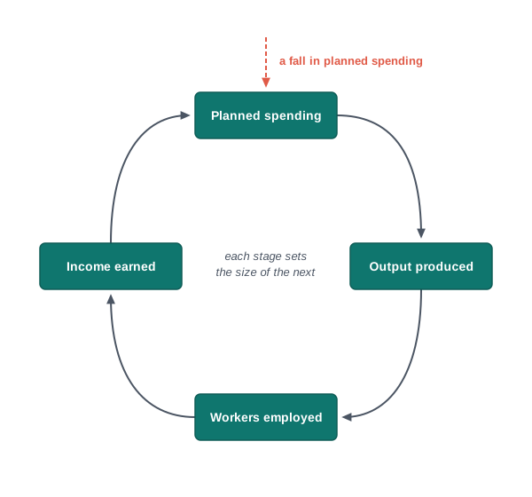
Fig. 2.0 – The spending, output and employment chain.
2.1 The Keynesian Model Of Income Determination
An economy has at any moment a given stock of factories, machinery, land and workers. Nothing in that stock prevents it from being used fully. Yet economies work below their capacity again and again: goods lie unsold in warehouses, plants run for part of the day only, and workers who are willing to work at the going wage cannot find jobs.
The problem this chapter takes up is therefore a problem of use rather than of scarcity of resources alone. What decides how much of an economy’s capacity is actually put to work in the short run? The tool economics uses on that question is a model of income determination — a set of relations showing the level of income at which the plans of buyers and the plans of producers are consistent with one another. The model set out here is the simple Keynesian model, and its answer is that this level is settled by demand.
2.1.1 The Central Proposition Of The Model
The cornerstone of the Keynesian model is that in the short run the level of income, output and employment in an economy depends on aggregate spending, that is, on the demand of the community as a whole for goods and services.
The chain of reasoning is short. The more that households and firms plan to spend, the larger is the quantity of goods and services that can be sold. The more that can be sold, the more firms will produce. The more they produce, the more workers they must employ. And the more workers they employ, the larger is the income earned in the economy. Demand calls forth output, and output calls forth income. Fig. 2.0 sets out this chain.
The chief feature of the theory is that it explains the level of income and employment whether or not the economy is working at full employment. Nothing in the model guarantees that the income so determined will be the full employment income. It may settle below that level and stay there, which is precisely what the theory was framed to explain.
2.1.2 Assumptions Of The Simple Keynesian Model
A model is a deliberate simplification, and this one is built on a small set of assumptions. Each of them is made for a reason, and knowing the reason is as important as knowing the assumption.
- Short period — the stock of capital, the technique of production and the size of the labour force are all taken as given. A rise in demand is therefore met by working the existing capacity harder and not by building fresh capacity.
- Constant prices — the price level is assumed to stay unchanged so long as the economy is below full employment. Any rise in the money value of output can then be read directly as a rise in real output and in employment.
- Excess production capacity — plants lie partly idle and workers are available for hire, so producers can raise output in response to demand without running into shortages of factors.
- Closed economy — exports and imports are left out of account, so no part of the country’s demand leaks abroad and no part of its supply is met from abroad.
- No government — taxes, government spending and transfers are assumed away, leaving a two-sector economy of households and firms in which aggregate demand consists of consumption expenditure and investment expenditure alone.
- Linear consumption function and autonomous investment — households are taken to spend a constant fraction of every additional rupee of income, and planned investment is taken as fixed whatever the level of income. Both keep the arithmetic of the model simple.
These assumptions strip the economy down, but they do not stand the argument on its head. When government activity and foreign trade are put back in, the conclusions of the simple model are qualified and not reversed: income, output and employment in the short run still depend on aggregate spending.
2.1.3 Desired (Ex Ante) And Effective (Ex Post) Demand
Aggregate demand in the theory of income determination always means planned demand — what buyers would like to spend at a given level of income, before the period of production is over. Economists mark such planned magnitudes with the Latin phrase ex ante, meaning ‘beforehand’.
What is actually bought when the period ends is a different quantity, and is described as ex post, meaning ‘afterwards’. The demand that is actually realised in this way is called effective demand.
Planned demand and actual demand need not agree, either in total or in any single component. Suppose firms produce a large output expecting brisk sales, and buyers spend less than expected. The goods that are not taken off the market do not vanish; they are added to the firms’ own stocks, and that addition is counted as investment by the firms. Actual investment therefore turns out to be larger than planned investment, and actual spending larger than planned spending. The two are equal only when the expectations of producers are exactly fulfilled — that is, only at equilibrium.
The gap between what is produced and what is bought, and the unintended stock that fills it, are shown in Fig. 2.1.
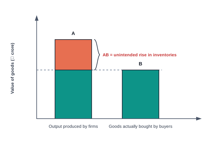
Fig. 2.1 – Unintended inventories when desired demand falls short of output.
The main points of difference between the two are set out below.
The model can now be built. Since planned spending is what drives income, the next step is to see what that spending consists of and how each part of it behaves.
2.2 Aggregate Demand And Aggregate Supply
To say that income is settled by demand is not yet to say very much. Demand has to be measured, and it has to be measured against something. The Keynesian model therefore works with two aggregates: the total that buyers plan to spend on the output of the economy, and the total value of the output that producers place before them.
The first of these is aggregate demand and the second is aggregate supply. Both are measured in money for a stated period of time, usually a year, and both are measured for the economy as a whole rather than for any single market.
2.2.1 Components Of Aggregate Demand
Aggregate demand is the desired or planned spending of the community on domestically produced goods and services. It is a schedule rather than a single number, since the amount buyers plan to spend is itself different at different levels of income.
Four groups of buyers make claims on the output of an economy: households buying goods for consumption, firms buying capital goods, the government buying goods and services for public purposes, and foreign buyers purchasing exports. Adding the planned spending of the four groups gives aggregate demand for the period.
\[AD = C + I + G + (X - M)\]
Here \(AD\) is aggregate demand, \(C\) is planned consumption expenditure by households, \(I\) is planned investment expenditure by firms, \(G\) is planned government expenditure and \((X - M)\) is net exports, exports minus imports. Every term is a money figure for the period, measured in ₹ crore. The total is read as the value of output that buyers intend to take off the market during the period.
The four components are as follows.
- Household consumption expenditure (\(C\)) — planned spending by households on goods and services meant for direct satisfaction of wants, such as food, clothing, fuel and services of every kind. It is the largest component in most economies and depends chiefly on the level of income.
- Investment expenditure (\(I\)) — planned spending by producers on capital goods such as plant, machinery and factory buildings, on additions to stocks of goods, and by households on new residential houses. It adds to the productive capacity of the economy.
- Government expenditure (\(G\)) — planned spending by the government on goods and services, from roads and schools to the salaries of public servants. It is decided by policy rather than by the level of income.
- Net exports (\(X - M\)) — the excess of what foreign buyers spend on the country’s exports over what residents spend on imports. Imports are deducted because aggregate demand measures demand for goods produced at home.
The shares of these four components in total planned spending are shown in Fig. 2.2.
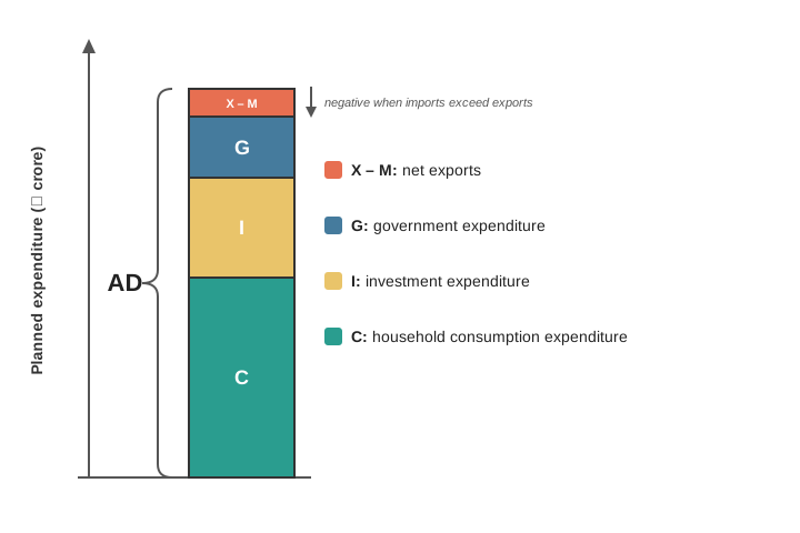
Fig. 2.2 – The four components of aggregate demand.
2.2.2 Aggregate Demand In A Two-Sector Economy
The simple model works with a closed economy in which the government is left out. Exports and imports then disappear from the expression, and so does government expenditure, leaving two components only.
\[AD = C + I\]
Consumption expenditure is the desired spending of households on consumer goods and services. Investment expenditure is the desired spending of producers on capital goods — tools, plant, machinery and factory buildings — together with additions to inventories and the purchase of new residential houses by households.
The two are kept apart because they are decided in quite different ways. Consumption is decided by a very large number of households and moves closely with income. Investment is decided by a much smaller number of firms and turns on the expected profitability of adding to capital, which is why the two are studied separately in Sections 2.3 and 2.5.
2.2.3 Aggregate Supply
Against planned spending stands the output actually placed on the market. Aggregate supply is the money value of all the goods and services produced in the economy during the period.
Producing output generates income of exactly the same amount, because the whole value of output is paid out as rent, wages, interest and profit to the owners of the factors that produced it. Aggregate supply and national income are therefore two names for one magnitude. Income in turn is either spent on consumption or saved, so aggregate supply can be written as the sum of the two.
\[AS = Y = C + S\]
Here \(AS\) is aggregate supply, \(Y\) is national income and \(S\) is saving, all measured in ₹ crore for the period. The expression says that whatever is produced is earned, and whatever is earned is either consumed or set aside.
This identity gives aggregate supply a convenient diagrammatic form. If income is measured along the X-axis and aggregate supply along the Y-axis, aggregate supply is shown by a straight line drawn from the origin at an angle of 45°, as in Fig. 2.3. At every point on that line the height above the X-axis equals the distance along it, which is exactly the statement that the value of output equals the income it creates.
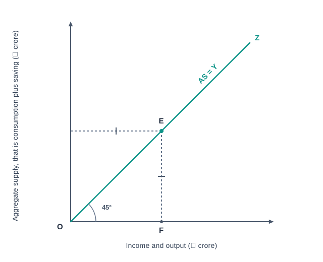
Fig. 2.3 – Aggregate supply as the 45° line.
The two aggregates are set against each other throughout the chapter, and the main points of difference between them are given below.
Of the two, aggregate supply needs no further explanation: it is simply the 45° line. Aggregate demand does, because its two components behave in quite different ways. The next section takes up the larger of them, household consumption.
2.3 Propensity To Consume
Of the two components of aggregate demand in a two-sector economy, consumption is the larger. It is also the more regular, because it is tied to something that can be observed and measured: the income of households. Investment, by contrast, depends on expectations of profit, which are far harder to pin down.
The question this section answers is therefore a question of behaviour. When the income of a community rises by a given amount, how much of that amount comes back into the market as spending on consumer goods, and how much is withheld? The relation that answers it is the consumption function.
2.3.1 The Consumption Function
The amount a household plans to spend on consumption depends on many things — the rate of interest, its holding of wealth and liquid assets, its expectations about future income, the stock of durable goods it already owns, and the ease with which it can borrow. Of all these, income is much the most important, and the simple model treats the others as given.
The functional relation between planned consumption expenditure and income is called the consumption function, or the propensity to consume.
Consumption does not fall to nothing when income falls to nothing. A household without income still eats, still pays for fuel and still buys clothing, meeting the cost by borrowing or by drawing down past savings. The same is true of an economy as a whole. This minimum level of spending, which is incurred even at zero income and is therefore not a function of income, is called autonomous consumption. The rest of consumption expenditure varies with income and is called induced consumption.
Taking the relation to be a straight line, as this chapter does throughout, the consumption function can be written in a form that separates the two parts. It states the total that households plan to spend at any level of income.
\[C = a + cY\]
Here \(C\) is planned consumption expenditure and \(Y\) is income, both measured in ₹ crore for the period. The intercept \(a\) is autonomous consumption, a positive constant that must be incurred even at zero income, and \(c\) is the fraction of any additional income that is consumed, which is the slope of the line. The term \(cY\) is induced consumption. The expression is read as a rule: begin with \(a\), and add \(c\) out of every rupee of income earned.
Plotted on a diagram with income on the X-axis and consumption on the Y-axis, this relation gives an upward sloping straight line that starts above the origin, as shown in Fig. 2.4. The 45° line is drawn along with it, because at every point on that line consumption would exactly equal income, and comparing the two lines shows at a glance whether households are saving or dissaving.
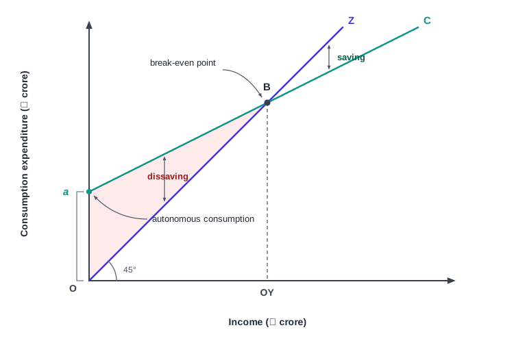
Fig. 2.4 – The consumption curve and the break-even point.
The income at which the consumption curve cuts the 45° line is the break-even point. At that level of income the whole of income is consumed and nothing is saved. To the left of it consumption exceeds income and the community is dissaving; to the right of it consumption falls short of income and the community is saving.
2.3.2 Average Propensity To Consume
Two measures are used to describe the propensity to consume. The first asks what proportion of a given income is spent on consumption.
The average propensity to consume measures the weight of consumption in income as a whole. It compares two totals, not two changes.
\[APC = \dfrac{C}{Y}\]
Here \(C\) is total consumption expenditure and \(Y\) is total income, both in ₹ crore. The result is a pure number with no unit, and is read as the part of one rupee of income that is spent on consumption. An APC of 0.90 means that ninety paise in every rupee of income is consumed and ten paise saved. Unlike the marginal measure that follows, APC can exceed one, and does so at every level of income below the break-even point, where the community consumes more than it earns.
2.3.3 Marginal Propensity To Consume
The second measure asks a different question, and it is the one that matters for the theory of income determination: of an addition to income, how much is spent?
The marginal propensity to consume looks only at the increment. It is the fraction \(c\) that appears in the consumption function, and it is the slope of the consumption curve.
\[MPC(c) = \dfrac{\Delta C}{\Delta Y}\]
Here \(\Delta C\) is the change in total consumption expenditure and \(\Delta Y\) the change in income, both in ₹ crore. The result is again a pure number. It always lies between zero and one, written \(0 < c < 1\), because an addition to income is never wholly ignored and never wholly spent: part of it is consumed and the rest saved.
The two measures are set out together in Table 2.1 for an economy whose consumption function is \(C = 40 + 0.8Y\).
Two things stand out from the table. The average propensity to consume falls steadily as income rises, from 1.20 to 0.87, because the fixed amount of autonomous consumption forms a smaller and smaller part of a growing income. The marginal propensity to consume stays at 0.80 throughout, because the consumption function is a straight line and its slope is the same everywhere. Both propensities can also be read off the diagram, as Fig. 2.5 shows.
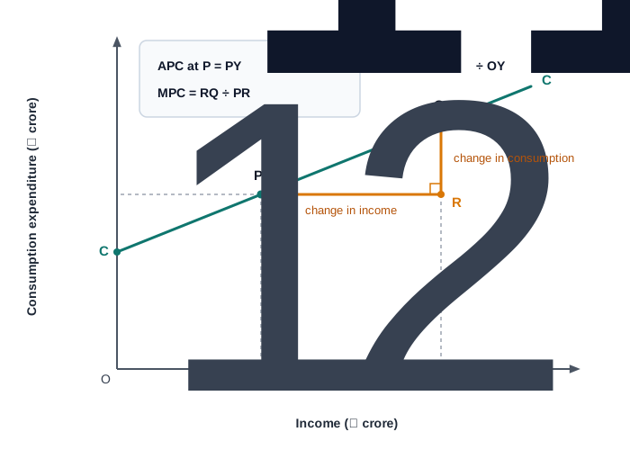
Fig. 2.5 – Measuring the average and marginal propensity to consume.
The main points of difference between the two propensities are set out below.
Both measures are worked out in SE 2.1 from a pair of observations, and in SE 2.2 from the consumption function itself.
2.3.4 Properties Of The Consumption Curve
Taken together, the two propensities give the consumption curve its shape, and four properties follow.
- Positive slope — consumption rises as income rises, because households with larger incomes buy more goods and services. The curve therefore slopes upward from left to right.
- Positive intercept — the curve begins above the origin, because autonomous consumption has to be met even at zero income out of borrowing or past saving.
- Slope less than unity — consumption rises by less than income, because part of any addition to income is saved. The curve is therefore flatter than the 45° line, and MPC lies between zero and one.
- A single break-even point — since the curve starts above the 45° line and is flatter than it, the two must cross once. To the left of the crossing there is dissaving and to the right there is saving.
A straight line consumption function has been assumed here so that the marginal propensity to consume is the same at every level of income. In practice it may fall as income rises, since people tend to consume a decreasing proportion of their additional income; the consumption function is then a curve rather than a line, but the Keynesian argument holds in either case.
The fourth property points directly to the next section. Whatever part of income is not consumed is saved, so a statement about consumption is at the same time a statement about saving.
2.4 Propensity To Save
Income has only two destinations. Whatever part of it is not spent on consumption is saved, and whatever part is not saved is spent. The two are joined at the hip, so a community that has settled how much it will consume has, by that very act, settled how much it will save.
This makes the propensity to save the exact counterpart of the propensity to consume. It is worth studying separately all the same, because in the theory of income determination it is saving that measures the leak — the part of income earned that is not returned to the market as demand.
2.4.1 The Saving Function
Saving is that part of income which is not spent on consumption. For the economy of a period, it is defined by subtraction.
\[S = Y - C\]
Here \(S\) is saving, \(Y\) is income and \(C\) is consumption expenditure, all measured in ₹ crore for the period. The expression is read as a residue: saving is what income leaves behind once consumption has been met.
Since consumption depends on income, saving must depend on income as well. Keynesian economics therefore treats saving, like consumption, as a function of income, and the relation between the two is the saving function or the propensity to save.
The saving function can be obtained from the consumption function by subtraction. If consumption is \(C = a + cY\), then saving is what is left of income after that spending has been made.
\[S = Y - (a + cY) = -a + (1 - c)Y\]
Here \(-a\) is the negative intercept, equal to the autonomous consumption that must be financed at zero income, and \((1 - c)\) is the fraction of any addition to income that is not consumed. For the economy of Table 2.1, whose consumption function is \(C = 40 + 0.8Y\), the saving function is \(S = -40 + 0.2Y\).
Drawn on a diagram, the saving function is an upward sloping straight line that begins below the origin, as Fig. 2.6 shows. It lies below the X-axis at low levels of income, where the community consumes more than it earns, cuts the axis at the break-even level of income, and lies above it thereafter.
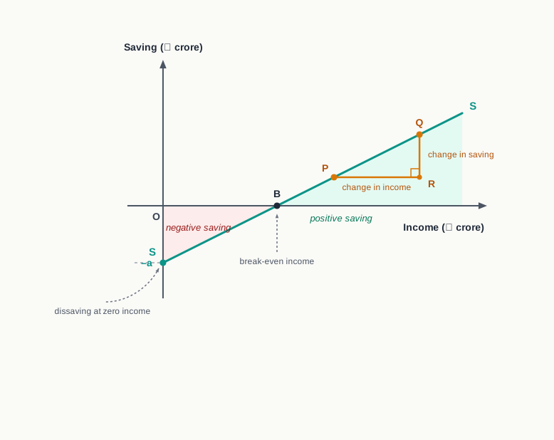
Fig. 2.6 – The saving curve.
2.4.2 Average Propensity To Save
As with consumption, two measures are used. The first states the proportion of a given income that is saved.
The average propensity to save compares two totals.
\[APS = \dfrac{S}{Y}\]
Here \(S\) is total saving and \(Y\) is total income, both in ₹ crore. The result is a pure number without unit, read as the part of one rupee of income that is set aside. An APS of 0.10 means ten paise in every rupee is saved. Below the break-even level of income APS is negative, since saving itself is negative there.
2.4.3 Marginal Propensity To Save
The second measure looks at the increment alone: of an addition to income, how much is withheld from the market?
The marginal propensity to save is the slope of the saving curve, and is written \(s\).
\[MPS(s) = \dfrac{\Delta S}{\Delta Y}\]
Here \(\Delta S\) is the change in saving and \(\Delta Y\) the change in income, both in ₹ crore. The result is a pure number lying between zero and one, since part of any addition to income is consumed and only the rest is saved. Table 2.2 sets out saving and the two propensities to save for the same economy used in the previous section.
Saving is negative up to an income of ₹200 crore, zero at that income and positive beyond it. The average propensity to save rises as income grows, while the marginal propensity to save stays at 0.20, since the saving curve is a straight line. The main points of difference between the two measures are set out below.
2.4.4 Relationship Between The Four Propensities
Since income is either consumed or saved, the two average measures must together account for the whole of income, and the two marginal measures for the whole of any addition to it.
Income is disposed of in two ways:
\[Y = C + S\]
Dividing every term by \(Y\) gives the first relationship.
\[\dfrac{C}{Y} + \dfrac{S}{Y} = 1 \quad \therefore \quad APC + APS = 1\]
An addition to income is disposed of in the same two ways:
\[\Delta Y = \Delta C + \Delta S\]
Dividing every term by \(\Delta Y\) gives the second relationship.
\[\dfrac{\Delta C}{\Delta Y} + \dfrac{\Delta S}{\Delta Y} = 1 \quad \therefore \quad MPC + MPS = 1\]
Both results are pure numbers and hold at every level of income. They are useful in two ways. Either measure of a pair can be found when the other is known, so that \(APC = 1 - APS\) and \(MPS = 1 - MPC\); and they supply a quick check on any numerical, since a set of answers in which APC and APS fail to add to one must contain an error. The working of both relationships is shown in SE 2.3 and SE 2.4.
2.4.5 Derivation Of The Saving Curve
Because saving is the gap between income and consumption, the saving curve can be drawn directly from the consumption curve without any fresh information. The method is shown in the two panels of Fig. 2.7.
The upper panel carries the consumption curve and the 45° line. Since every point on the 45° line measures income, the vertical distance between that line and the consumption curve at any level of income is precisely saving at that income. Transferring that distance to the lower panel, level by level, traces out the saving curve. Where the consumption curve lies above the 45° line the distance is carried below the horizontal axis as dissaving; where the two curves cross, saving is zero; and beyond the crossing the gap widens steadily, which is why the saving curve slopes upward.
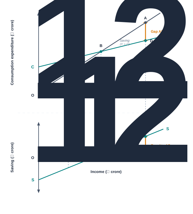
Fig. 2.7 – Derivation of the saving curve from the consumption curve.
The consumption and saving functions together account for the whole of household behaviour in this model. The other component of aggregate demand, investment, is decided elsewhere, and is taken up next.
2.5 Investment Expenditure
Consumption expenditure is decided by millions of households on the basis of income, which is why it can be written as a stable function. The other component of aggregate demand is decided by a much smaller number of producers on the basis of what they expect to earn from an addition to their capital, and expectations are not stable in the same way. Investment is therefore the restless element in aggregate demand.
Its importance to the model lies in this restlessness. A change in investment is the usual disturbance that sets income moving, and much of the rest of the chapter traces what follows from such a change.
In modern macroeconomic analysis, investment is taken in the sense of real investment — an addition to the stock of physical capital in the economy — and not in the sense in which the word is used in ordinary speech.
The items that count as investment in this sense are of four kinds.
- Plant, machinery and equipment — the tools with which goods are produced. Spending on them adds directly to the productive capacity of the economy.
- New structures — factory buildings, offices and other business construction, which are as much a part of the capital stock as the machinery they house.
- New residential houses — treated as investment even when bought by a household, because a house yields its services over many years rather than being used up in the period.
- Additions to inventories — stocks of raw materials, goods in process and finished goods held by firms. An addition to stocks is output produced but not consumed, and is therefore investment, whether the firm intended it or not.
2.5.1 Private And Public Investment
Investment may first be classified by who undertakes it.
Private investment is the expenditure incurred by private entrepreneurs on the purchase of capital goods such as plant, machinery, factories, offices and inventories. It is motivated by the profit that the entrepreneur expects the new capital to earn, and it is undertaken only when that expected profit is judged worth the outlay.
Public investment is the investment undertaken by the government. Roads, dams, schools, colleges, hospitals, water supply, transport and housing are built by governments in most countries, and such investment is guided largely by public welfare rather than by profit.
The main points of difference between the two are given below.
In the analysis of income and output that follows, the discussion is confined to private investment, since the activities of the government have been assumed away.
2.5.2 Autonomous And Induced Investment
Investment may also be classified by what makes it change, and this second classification is the one the model actually uses.
Induced investment is investment undertaken as a result of a change in the level of income. A rise in income raises the demand for consumer goods; to produce more consumer goods, firms need more capital; and so investment rises with income. Induced investment is therefore income-elastic, and is shown by an upward sloping curve, as in panel (i) of Fig. 2.8.
Autonomous investment is investment that is not affected by a change in the level of income or output. It is independent of income and is therefore income-inelastic, shown by a horizontal line parallel to the X-axis, as in panel (ii) of Fig. 2.8. The same amount is undertaken whether income is large or small.
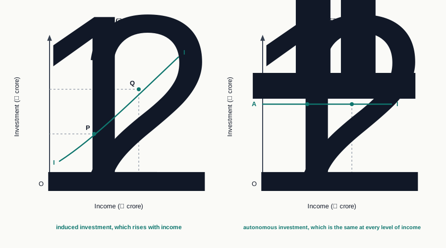
Fig. 2.8 – Induced and autonomous investment.
Most investment made by governments is autonomous, and a good deal of private investment is induced. The simple Keynesian model, however, takes all investment to be autonomous. The reason is one of method rather than of fact: if investment were allowed to rise with income at the same time as consumption does, it would be impossible to see clearly what a given change in demand does to income. Holding investment fixed isolates the effect that the model is built to display.
The main points of difference between the two are given below.
Both components of aggregate demand have now been set out: consumption, which rises with income but by less than income, and investment, which is taken as a fixed amount. Putting the two together against aggregate supply gives the equilibrium level of income, and that is the subject of the next section.
2.6 Determination Of Equilibrium Income And Output
Producers must decide how much to produce before they know how much will be bought. Most of the time the two magnitudes do not agree, and the disagreement shows itself in stocks that pile up unsold or run down faster than expected. Output is then revised, and revised again, until a level is reached at which producers find their expectations exactly fulfilled.
That level is the equilibrium level of income. It is not a level at which everybody is satisfied, and it need not be the level at which all the resources of the economy are employed. It is simply the level at which no producer has any reason to change what he is doing.
The equilibrium level of income can be located in two ways, and both give the same answer. The first sets total planned spending against total output; the second sets planned saving against planned investment.
2.6.1 Aggregate Demand–Aggregate Supply Approach
Aggregate demand in the two-sector economy is planned consumption plus planned investment. Its curve is obtained by adding the investment line to the consumption curve at every level of income — that is, by vertical summation. Since planned investment is autonomous and therefore the same at all levels of income, the C + I curve is parallel to the consumption curve and lies above it by a constant distance equal to investment.
Aggregate supply is the 45° line, along which the value of output equals the income it generates. Equilibrium is at the point where the two meet.
\[AD = AS\]
Here \(AD\) is planned aggregate demand and \(AS\) is aggregate supply, both in ₹ crore for the period. Written out in terms of their components, the condition becomes \(C + I = Y\). The income at which it holds is the equilibrium income; at any other income the plans of buyers and the plans of producers are inconsistent. The construction is shown in Fig. 2.9.
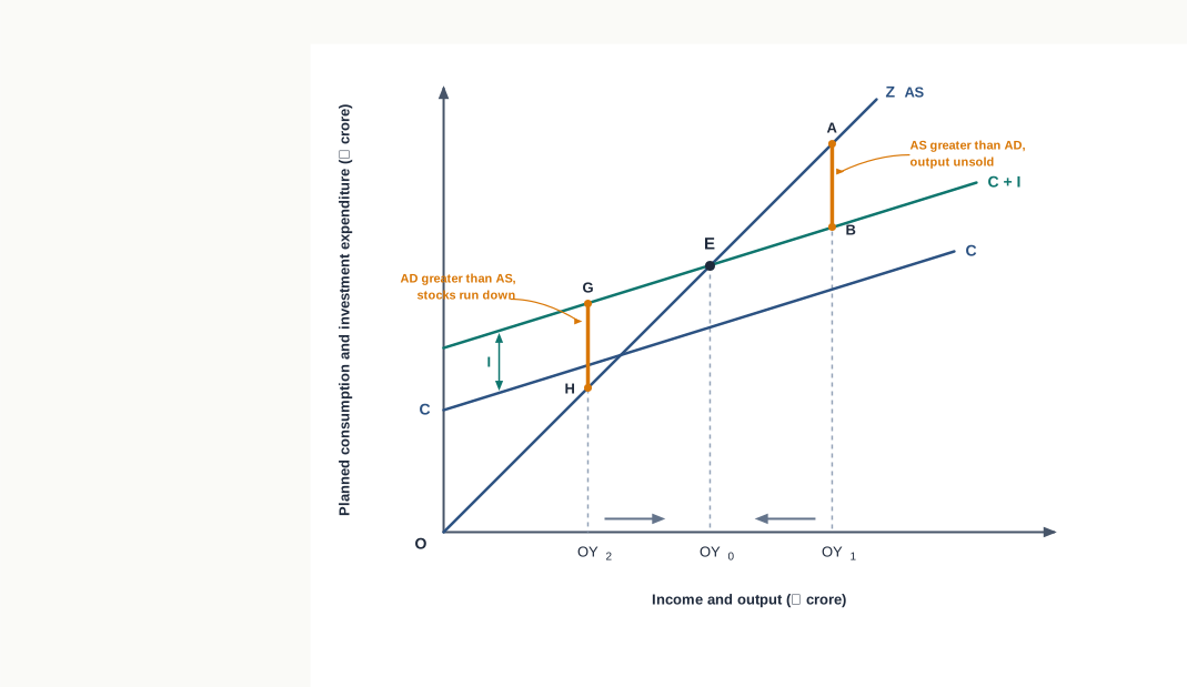
Fig. 2.9 – Equilibrium through aggregate demand and aggregate supply.
Consider a level of output larger than the equilibrium, such as OY1. Planned spending there, measured by BY1, falls short of the output produced, measured by AY1. Firms cannot sell the whole of what they have made, and the unsold quantity AB is added to their stocks. Faced with inventories they never meant to hold, they cut production; income and employment fall; and the process continues until income has fallen to OY0.
Now consider a level of output smaller than the equilibrium, such as OY2. Planned spending there, measured by GY2, exceeds the output produced, measured by HY2. The excess GH is met by selling out of stocks. Finding their inventories falling below the level they wish to hold, firms raise production, take on more workers and generate more income, and the process continues until income has risen to OY0.
At OY0 neither pressure exists. Buyers can carry out their spending plans in full and producers can sell exactly what they planned to produce, so output and income come to rest.
2.6.2 Saving–Investment Approach
The second approach follows from the first by simple substitution. Aggregate demand is consumption plus investment, and aggregate supply, being income, is consumption plus saving.
\[C + I = C + S\]
Cancelling consumption from both sides leaves the condition in its second form.
\[\therefore \quad I = S\]
Here \(I\) is planned investment and \(S\) is planned saving, both in ₹ crore. The condition is read as a balance between a withdrawal and an injection: saving is the part of income that households do not return to the market, and investment is the spending that firms add to it. Income comes to rest where the amount withheld is exactly the amount put back.
Diagrammatically, the saving curve slopes upward and the investment line is horizontal, since investment is autonomous. Equilibrium is where they cut, as in Fig. 2.10.
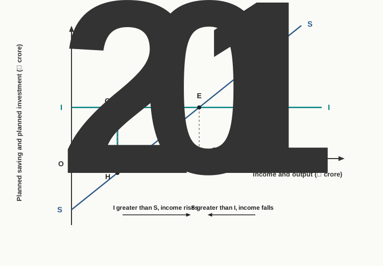
Fig. 2.10 – Equilibrium through saving and investment.
At an income larger than OY0, planned saving exceeds planned investment. Households are withholding more from the market than firms are putting back, so aggregate demand falls short of aggregate supply, stocks accumulate and firms cut production. Income, output and employment fall until saving has come down to the level of investment. At an income smaller than OY0 the position is reversed: planned investment exceeds planned saving, demand outruns production, stocks are run down and firms expand output until saving has risen to the level of investment.
The two approaches differ only in what is placed on the diagram, as set out below.
2.6.3 Adjustment Through Unplanned Inventories
The two diagrams state where the economy comes to rest, but they do not by themselves explain how it gets there. The agent of adjustment is the unplanned change in inventories, and the numerical schedule in Table 2.3 shows it at work in the economy whose consumption function is \(C = 40 + 0.8Y\) and whose planned investment is ₹60 crore.
At an output of ₹400 crore, buyers plan to spend ₹420 crore, which is ₹20 crore more than has been produced. The excess is met out of stocks; inventories fall below the level firms wish to hold; and firms expand production and employment to rebuild them. At an output of ₹600 crore, buyers plan to spend ₹580 crore, which is ₹20 crore less than has been produced. The unsold ₹20 crore of goods is added to stocks; inventories rise above the level firms wish to hold; and firms cut production, so income and employment fall. Only at ₹500 crore does planned spending exactly absorb the output produced, and there saving of ₹60 crore is exactly equal to investment of ₹60 crore.
The mechanism is worth stating in general terms, because it is the same in every case. An unplanned rise in inventories is a signal that demand has fallen short of output, and firms respond by producing less. An unplanned fall in inventories is a signal that demand has outrun output, and firms respond by producing more. Since prices are assumed fixed in the short run, quantity and not price does all the adjusting, and the quantity that adjusts is output — which is to say, income and employment.
Two conclusions follow from this section, and both matter for the rest of the chapter. First, the level of income is settled by the strength of aggregate demand, so a change in demand must change income. Second, nothing in the argument required that income to be the full employment income. The first conclusion leads to the investment multiplier, taken up next; the second leads to the problem of underemployment equilibrium, taken up in Section 2.8.
2.7 The Investment Multiplier
Section 2.6 established that a change in aggregate demand changes the equilibrium level of income. It did not say by how much. Common sense suggests that if firms spend ₹100 crore more on new plant, income should rise by ₹100 crore. The Keynesian model gives a more surprising answer: income rises by a multiple of the additional investment.
The reason is that spending does not stop where it starts. What one person spends becomes the income of another, who spends a part of it in turn, and so on. The tool that measures the total effect of this chain is the investment multiplier, and it occupies a central place in the modern theory of income and employment.
2.7.1 Meaning Of The Investment Multiplier
The multiplier compares two changes, and is written as their ratio.
\[K = \dfrac{\Delta Y}{\Delta I}\]
Here \(K\) is the investment multiplier, \(\Delta Y\) is the change in income and \(\Delta I\) the change in investment, both measured in ₹ crore. The result is a pure number with no unit, read as the number of times by which income changes for a given change in investment. If an addition of ₹100 crore to investment raises income by ₹500 crore, the multiplier is 5.
The word ‘increase’ in the definition should not mislead. The multiplier works in both directions: a fall in investment lowers income by a multiple amount in exactly the same way, and for exactly the same reason.
2.7.2 Working Of The Multiplier
Take the economy of Table 2.3, in equilibrium at an income of ₹500 crore with a marginal propensity to consume of 0.8, and suppose firms decide to spend an additional ₹20 crore on a new plant.
In the first round, the ₹20 crore is paid out to those who supply the machinery, materials, land and labour used in building the plant. Income in the economy rises by ₹20 crore, an amount equal to the investment itself. But this is not the end of the story. The people who have received the ₹20 crore spend a part of it on consumer goods, and how much they spend depends on the marginal propensity to consume. With MPC of 0.8, they spend ₹16 crore.
That ₹16 crore is spent on food, clothing and other goods, and becomes the income of the firms and workers who produce them, raising income by a further ₹16 crore in the second round. They in turn spend 0.8 of it, or ₹12.80 crore, in the third round. Each round is 0.8 of the one before it, so the additions to income grow steadily smaller, and the whole process is set out in Table 2.4.
The additions do not go on for ever in any practical sense, because a part of every round’s income is saved rather than passed on. Since the amounts shrink towards zero, their total is finite: an initial ₹20 crore of investment has raised income by ₹100 crore in all, and consumption by ₹80 crore. Fig. 2.11 shows the same series drawn to scale.
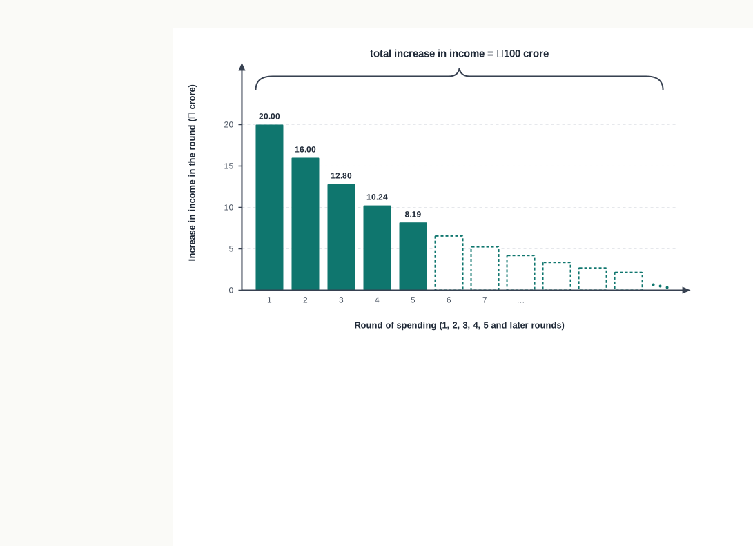
Fig. 2.11 – Successive rounds of income propagation.
2.7.3 Derivation Of The Multiplier Formula
The size of the multiplier can be obtained from the equilibrium condition itself. In the two-sector model, income equals consumption plus investment.
\[Y = C + I\]
If investment changes, income changes, and the change in income is made up of the change in consumption it induces together with the change in investment that began it.
\[\Delta Y = \Delta C + \Delta I\]
The change in consumption is the marginal propensity to consume times the change in income, since \(c\) is by definition the fraction of additional income that is consumed. Substituting \(\Delta C = c\Delta Y\) gives:
\[\Delta Y = c\Delta Y + \Delta I\]
\[\Delta Y - c\Delta Y = \Delta I\]
\[\Delta Y(1 - c) = \Delta I\]
Dividing both sides by \((1 - c)\) and then by \(\Delta I\) isolates the multiplier.
\[K = \dfrac{\Delta Y}{\Delta I} = \dfrac{1}{1 - c} = \dfrac{1}{1 - MPC}\]
Since \(MPC + MPS = 1\), the denominator \((1 - MPC)\) is the marginal propensity to save, and the multiplier can equally be written as its reciprocal.
\[K = \dfrac{1}{MPS} = \dfrac{1}{s}\]
Here \(c\) is the marginal propensity to consume and \(s\) the marginal propensity to save, both pure numbers. The result is read as the number of times income changes for a one-rupee change in investment, and it says that the multiplier depends on nothing except the way households divide additional income between spending and saving.
The same result can be shown on the income diagram. An increase in autonomous investment shifts the whole aggregate demand curve upward by the amount of the increase, and the new curve cuts the 45° line further to the right, as in Fig. 2.12. The horizontal distance between the two equilibrium levels of income is larger than the vertical shift of the curve, and that is the multiplier at work.
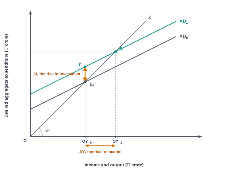
Fig. 2.12 – The multiplier on the income diagram.
2.7.4 Size Of The Multiplier And The Propensities
The formula shows that the size of the multiplier turns entirely on the marginal propensity to consume, and the relation is a direct one. A high MPC means that a large part of each round’s income is passed on as spending, so the later rounds stay large and the final rise in income is great. A low MPC means that most of each round’s income is withheld as saving, so the rounds die away quickly and the final rise is small. The same relation seen from the other side is an inverse one: the larger the marginal propensity to save, the smaller is the multiplier, since \(K\) is the reciprocal of MPS.
The two extreme values in the table mark the limits within which the multiplier must lie.
- When MPC is zero — the whole of any additional income is saved and nothing is passed on. The chain stops at the first round, income rises only by the investment itself, and the multiplier takes its lowest value of one.
- When MPC is one — the whole of any additional income is spent and nothing leaks away. No round is smaller than the one before it, the process never dies down, and the multiplier is infinite.
Neither extreme is found in practice, so the multiplier lies between one and infinity. It should be added that the multiplier is a two-way instrument. Just as an increase in investment raises income by a multiple amount, a fall in investment lowers income by a multiple amount, as each round of reduced spending cuts somebody else’s income and hence their spending in the round after.
The multiplier explains why a modest change in investment can move a whole economy, and why the change may be for the worse as easily as for the better. It also raises the question the chapter has so far avoided. If demand settles income, and income may settle anywhere, what becomes of full employment? That is the subject of the next section.
2.8 Full Employment And Unemployment
The model has now delivered an equilibrium level of income, and the equilibrium is a genuine one: at that income buyers can carry out their plans and producers have no reason to change their output. Nothing in the argument, however, said anything about the workers of the economy. Whether the labour force is fully employed at that income was never asked, and the answer is that it may or may not be.
This is the most important contention of Keynesian economics. The equilibrium level of income is settled by aggregate spending, and aggregate spending may be too small to buy the output that would keep every willing worker employed. An economy can therefore come to rest, and stay at rest, with resources lying idle.
2.8.1 The Concept Of Full Employment
Two qualifications are contained in that definition, and both must be stated.
- Full employment does not mean that everybody is employed — persons who are not willing to work at the prevailing wage rate are not employed, but neither are they unemployed in the sense used here. They have chosen not to offer their labour, and their choice is not a failure of the economy.
- Full employment is consistent with some unemployment — at any moment some workers are between jobs, moving from one place or one trade to another, or waiting while the demand for a particular product changes. Such frictional unemployment takes time to work itself out and is found even in a fully employed economy.
An economy in which only these two kinds of unemployment exist is described as fully employed. Full employment is therefore a statement about the willing, not about the whole population.
2.8.2 Voluntary And Involuntary Unemployment
In ordinary speech, a person who is not gainfully employed is called unemployed. Economics uses the word more narrowly, and separates two very different situations.
Voluntary unemployment refers to persons who are unemployed by their own choice. They may be unwilling to work because they have other means of support, or because they are not interested in any gainful job on offer at the prevailing wage. Since they are not offering their labour, it would be misleading to count them among the unemployed.
Involuntary unemployment refers to a situation in which people are able to work and willing to work at the prevailing wage rate, but are unable to find work. They are unemployed against their wish. It is this kind of unemployment that the theory of income and employment sets out to explain, because it is a failure of the economy rather than a choice of the individual.
The main points of difference between the two are given below.
2.8.3 Underemployment Equilibrium
If aggregate spending is not large enough to call forth the output that would employ the whole labour force, the economy settles at an income below the full employment income. That position has a name.
The position is shown in Fig. 2.13. The aggregate demand curve AD0 cuts the 45° line at E0, giving an equilibrium income of OY0. The full employment income is OYf, further to the right. The economy is at rest at OY0 and will stay there, because at that income planned spending exactly absorbs the output produced. The difference Y0Yf measures the output that is not produced and, with it, the workers who are not employed.
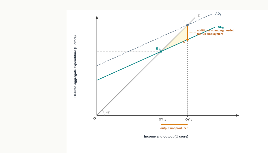
Fig. 2.13 – Underemployment equilibrium.
The remedy the diagram suggests is a rise in aggregate demand. If spending rises so that the demand curve moves up to AD1, the new equilibrium is at F and income is the full employment income OYf. Note that the upward shift AF required is smaller than the rise in income Y0Yf it produces, since the multiplier is at work here as everywhere else.
Three positions are therefore possible in this model. Aggregate demand may be exactly large enough to buy the full employment output, in which case the economy is in equilibrium at full employment. It may fall short of that amount, giving the underemployment equilibrium just described. Or it may exceed it, in which case output cannot rise any further, since all resources are already employed, and the pressure of demand spends itself on prices instead. The last two cases are the problems of excess demand and deficient demand, and they are taken up next.
2.9 Excess Demand And Deficient Demand
Full employment output is a ceiling. An economy cannot produce beyond it in the short run, because there are no further resources to draw upon; but it can very easily produce below it. Aggregate demand may therefore stand in one of two wrong relations to that ceiling — it may be more than enough to buy the full employment output, or less than enough.
Neither position corrects itself, and the two do quite different damage. Too much demand raises prices; too little destroys output and jobs. This section examines both, and the measures a government and a central bank use against them.
2.9.1 Excess Demand And The Inflationary Gap
When the economy is already working at full employment, this excess cannot be wiped out by producing more. Every worker who is willing to work is employed and every plant is in use, so output cannot rise. The extra spending meets an unchanged quantity of goods, shortages appear, and prices are pushed up. Excess demand therefore does not raise output and employment; it causes inflation.
The extent of the excess is measured by the inflationary gap.
Fig. 2.14 shows the position.
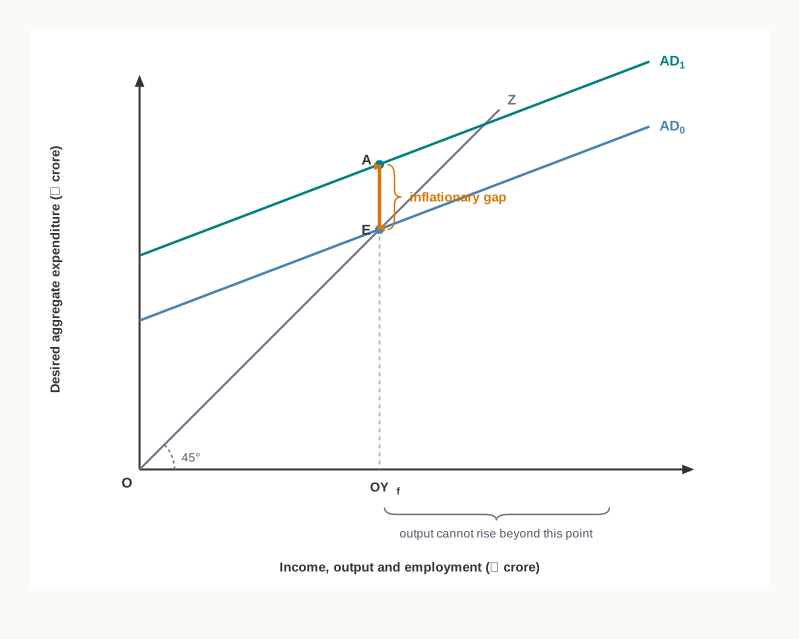
Fig. 2.14 – Excess demand and the inflationary gap.
Excess demand may arise from an increase in any component of aggregate demand.
- A rise in consumption expenditure — households with a higher propensity to consume spend a larger part of a given income, and demand rises without any rise in output.
- A rise in private investment — firms expecting good profits order more plant and machinery, adding to demand while the goods themselves take time to add to capacity.
- A rise in government expenditure not matched by taxation — the government adds to demand without withdrawing an equal amount of purchasing power from the public.
- A rise in exports — foreign buyers take a part of the domestic output, leaving less of it for buyers at home.
- An increase in the supply of money — with more money in the hands of the public and credit easier to obtain, spending rises.
2.9.2 Measures To Correct Excess Demand
Since the trouble is that aggregate demand exceeds the full employment output, the cure is to reduce aggregate demand by the amount of the inflationary gap. The instruments are of four kinds.
- Fiscal policy — the policy under which the government uses taxation, public expenditure and public borrowing to influence the economy.
- Taxation — new taxes may be imposed and the rates of existing taxes raised. Higher direct taxes reduce the disposable income of households and so their consumption expenditure, while higher taxes on business profits discourage investment spending.
- Public expenditure — the government curtails its own spending, particularly on unproductive and non-development items. A cut in government purchases of goods and services reduces aggregate demand directly.
- Public borrowing — large-scale borrowing from the public mops up purchasing power that would otherwise have been spent.
- Deficit financing — the practice of meeting a deficit by the creation of new money is cut down, since it adds directly to the spending power in the economy.
- Monetary policy — the policy under which the central bank controls the supply of money and the availability of credit.
- Bank rate and repo rate — raising the rate at which the central bank lends to commercial banks raises the rate of interest they charge their customers. Costlier credit reduces the consumption and investment expenditure that is financed by borrowing.
- Open market operations — the central bank sells government securities to the commercial banks and the public, drawing cash out of the banking system and reducing its capacity to lend.
- Cash reserve ratio and statutory liquidity ratio — raising these ratios obliges banks to hold a larger part of their deposits as reserves, which cuts the amount they can lend and hence the spending financed by bank credit.
- Increasing imports — buying goods from abroad adds to the supply available at home and so relieves the pressure of demand on domestic output.
- Increasing output — production may be raised where any slack remains, though in the short run this possibility is limited, which is why the measure works better over a longer period.
2.9.3 Deficient Demand And The Deflationary Gap
The opposite disorder is the one with which the chapter began.
Here output can adjust, and it does. Firms are left with goods they cannot sell, inventories pile up, production is cut back and workers are laid off. Income and employment fall, and the economy comes to rest at an underemployment equilibrium. Prices fall as well, since sellers are competing for a demand that is not there. Deficient demand thus carries the potentiality of deflation, and the gap that measures it takes its name from that.
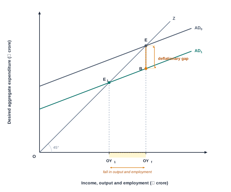
Fig. 2.15 – Deficient demand and the deflationary gap.
The causes of deficient demand are the mirror images of those listed earlier: a fall in consumption expenditure as households save a larger part of their income, a fall in private investment, a cut in government expenditure not matched by a cut in taxes, a fall in exports, and a contraction in the supply of money and bank credit.
2.9.4 Measures To Correct Deficient Demand
The measures used against deficient demand are the same instruments worked in the opposite direction, and the aim is to raise aggregate demand by the amount of the deflationary gap.
- Fiscal policy
- Taxation — direct taxes on personal incomes and on business profits are reduced. A cut in income tax leaves households with larger disposable incomes to spend, and a cut in taxes on profits improves the incentive to invest.
- Public expenditure — the government increases its own spending, particularly on public works such as roads, bridges and railway lines, and on welfare measures such as unemployment relief and old-age pensions. This is the most direct way of adding to demand.
- Public borrowing — borrowing from the public is discouraged, so that purchasing power is left in the hands of the people who will spend it.
- Deficit financing — the government may deliberately spend beyond its revenue, since this adds to its ability to spend and so to aggregate demand.
- Monetary policy
- Bank rate and repo rate — the central bank lowers the rate at which it lends to commercial banks, so that the interest they charge falls and borrowing for consumption and investment becomes cheaper.
- Open market operations — the central bank buys government securities from banks and the public, putting cash into the banking system and enlarging its capacity to lend.
- Cash reserve ratio and statutory liquidity ratio — these ratios are lowered, freeing a larger part of bank deposits for lending.
- Export promotion — subsidies and tax concessions to exporters raise the demand for domestic goods in foreign markets, which adds to aggregate demand at home.
The two disorders and their treatment are set out together below.
The chapter has come full circle. It began with an economy whose factories stood idle although nothing was wrong with the factories, and it ends with the reason and the remedy: what was missing was demand, and demand is something a government and a central bank can act upon.
2.10 Summary
- The cornerstone of the simple Keynesian model is that in the short run the level of income, output and employment in an economy depends on aggregate spending. Demand calls forth output, and output calls forth income.
- The model rests on six assumptions, each made for a reason.
- A short period, in which capital, technique and the labour force are given.
- A constant price level, so that a change in the money value of output is a change in real output.
- Excess production capacity, so that output can rise when demand rises.
- A closed economy, with no exports or imports.
- No government, leaving a two-sector economy of households and firms.
- A linear consumption function and autonomous investment.
- Desired or ex ante demand is what buyers plan to spend; effective or ex post demand is what they actually spend. The two are equal only at equilibrium, because unsold goods are counted as unintended inventory investment.
- Aggregate demand is total planned spending on domestic output, \(AD = C + I + G + (X - M)\), where \(C\) is consumption expenditure, \(I\) investment expenditure, \(G\) government expenditure and \((X - M)\) net exports. In a two-sector closed economy it reduces to \(AD = C + I\).
- Aggregate supply is the money value of output produced, and equals national income. Since income is either consumed or saved, \(AS = Y = C + S\), which is why aggregate supply is drawn as a 45° line from the origin.
- The consumption function shows planned consumption as a function of income, \(C = a + cY\), where \(a\) is autonomous consumption, incurred even at zero income, and \(cY\) is induced consumption, \(c\) being the marginal propensity to consume.
- The average propensity to consume is the proportion of total income consumed, \(APC = \dfrac{C}{Y}\), where \(C\) is total consumption and \(Y\) total income. It falls as income rises and may exceed one below the break-even income.
- The marginal propensity to consume is the proportion of an addition to income that is consumed, \(MPC = \dfrac{\Delta C}{\Delta Y}\), where \(\Delta C\) and \(\Delta Y\) are the changes in consumption and in income. It is the slope of the consumption curve and always lies between zero and one, \(0 < c < 1\).
- The break-even point is the level of income at which the consumption curve cuts the 45° line, so that the whole of income is consumed and saving is zero. Below it there is dissaving and above it there is saving.
- Saving is income not consumed, \(S = Y - C\). Derived from the consumption function it becomes \(S = -a + (1 - c)Y\), where \(-a\) is dissaving at zero income and \((1 - c)\) is the marginal propensity to save.
- The average propensity to save is the proportion of total income saved, \(APS = \dfrac{S}{Y}\), where \(S\) is total saving. It is negative below the break-even income, zero at it and positive above it.
- The marginal propensity to save is the proportion of an addition to income that is saved, \(MPS = \dfrac{\Delta S}{\Delta Y}\). It is the slope of the saving curve and lies between zero and one.
- Since income and every addition to it are divided between consumption and saving, \(APC + APS = 1\) and \(MPC + MPS = 1\) at every level of income. Either measure of a pair can therefore be found when the other is known.
- Investment means real investment — an addition to the stock of physical capital, including new plant, machinery, structures, residential houses and additions to inventories. It is classified in two ways.
- Private investment, undertaken by firms for profit, and public investment, undertaken by the government for public welfare.
- Autonomous investment, which does not vary with income and is drawn as a horizontal line, and induced investment, which varies directly with income and is drawn as an upward sloping curve.
- Equilibrium income is the level at which aggregate demand equals aggregate supply, \(Y = C + I\), so that producers can sell exactly what they plan to produce and have no reason to change output. On the diagram it is where the \(C + I\) curve cuts the 45° line.
- The same condition can be written as \(S = I\), planned saving equal to planned investment, since the leakage from the circular flow is then exactly matched by the injection into it. Both approaches give the same equilibrium level of income.
- Adjustment to equilibrium works through unplanned inventories. An unintended rise in stocks makes firms cut production, so income falls; an unintended fall in stocks makes them raise production, so income rises. With prices fixed, output and employment do all the adjusting.
- The investment multiplier is the multiple by which income rises when investment rises, \(K = \dfrac{\Delta Y}{\Delta I}\), where \(\Delta Y\) is the change in income and \(\Delta I\) the change in investment. It works because what one person spends becomes another person’s income.
- The multiplier depends only on how additional income is divided, \(K = \dfrac{1}{1 - c} = \dfrac{1}{MPS}\). It varies directly with the marginal propensity to consume and inversely with the marginal propensity to save, and its value lies between one and infinity. It works in reverse as well, so a fall in investment lowers income by a multiple amount.
- Full employment is the situation in which all those willing to work at the prevailing wage rate are employed. It does not mean that everybody is employed, and it is consistent with the frictional unemployment of workers who are between jobs.
- Voluntary unemployment is unemployment by choice and is not counted; involuntary unemployment is the position of those able and willing to work at the prevailing wage who cannot find work, and it is the kind the theory explains.
- Underemployment equilibrium is an equilibrium reached below the full employment level of income, at which resources lie idle although demand equals supply and the economy has no tendency to move.
- Excess demand is the amount by which aggregate demand exceeds the full employment output, and the inflationary gap measures it. Output cannot rise, so the excess raises prices, and the remedy is to reduce aggregate demand.
- Fiscal measures — raise taxes, cut public expenditure, increase public borrowing and reduce deficit financing.
- Monetary measures — raise the bank rate and repo rate, sell government securities in the open market and raise the cash reserve ratio.
- Other measures — increase imports and, so far as capacity allows, increase output.
- Deficient demand is the amount by which aggregate demand falls short of the full employment output, and the deflationary gap measures it. Output, employment and prices all fall, and the remedy is to raise aggregate demand.
- Fiscal measures — reduce taxes, increase public expenditure, discourage public borrowing and resort to deficit financing.
- Monetary measures — lower the bank rate and repo rate, buy government securities in the open market and lower the cash reserve ratio.
- Other measures — promote exports through subsidies and tax concessions.
- The four propensities, which carry most of the chapter’s arithmetic, are set out together below.
2.11 Points to Ponder
- A household that saves more is thought prudent. Yet if every household in a country decided to save more at the same time, planned saving would run ahead of planned investment and income would fall. Can thrift be a virtue for one family and a vice for the economy at the same moment, and what would settle the question?
- The model assumes that prices stay fixed while output adjusts. In an economy where the prices of food and fuel move quickly, is it reasonable to expect a rise in demand to show itself wholly in output and employment, or would part of it go into prices from the very beginning?
- The multiplier of the closed model treats saving as the only leakage. If a large part of every additional rupee of income is spent on imported goods, how much of the benefit of a rise in domestic investment stays within the country, and does that strengthen or weaken the case for such a policy?
- Underemployment equilibrium persists because demand is too small to employ everyone at the prevailing wage. Would a general cut in wages put those workers back to work, or would it cut incomes and with them the very demand that is missing? Which of the two arguments do you find stronger, and on what grounds?
- Excess demand can be reduced by raising taxes or by cutting public expenditure. Both withdraw the same amount of spending from the economy, but not from the same people. Who bears the cost in each case, and should that consideration decide the choice between them?
- The Keynesian remedy assumes that idle capacity is waiting to be used. Where output is held back instead by shortages of power, transport or trained workers, would a rise in aggregate demand raise production, raise prices, or do both — and what evidence would you look for to tell which was happening?
2.12 Objective Questions
- In a two-sector closed economy, aggregate demand consists of: [1]
- consumption expenditure and government expenditure
- consumption expenditure and investment expenditure
- investment expenditure and net exports
- consumption expenditure, investment expenditure and net exports
- Assertion (A): The average propensity to consume may be greater than one, but the marginal propensity to consume cannot be. Reason (R): Below the break-even income a community consumes more than it earns by drawing on past savings, whereas an addition to income is always divided between consumption and saving. [1]
- Both A and R are true, and R is the correct explanation of A.
- Both A and R are true, but R is not the correct explanation of A.
- A is true but R is false.
- A is false but R is true.
- Fill in the blank: The level of income at which the consumption curve cuts the 45° line, so that saving is zero, is called the ______ point. [1]
- State whether the following statement is true or false: An economy that has settled at an underemployment equilibrium will move to full employment of its own accord. [1]
- Match the items in Column 1 with those in Column 2. [1]
| Column 1 | Column 2 |
|---|---|
| a. Investment multiplier | i. \(\dfrac{C}{Y}\) |
| b. Marginal propensity to save | ii. \(\dfrac{\Delta S}{\Delta Y}\) |
| c. Average propensity to consume | iii. \(\dfrac{1}{1 - MPC}\) |
2.13 Check Your Concepts
- Distinguish between desired (ex ante) demand and effective (ex post) demand. [2]
- In an economy the consumption function is \(C = 50 + 0.75Y\) and planned investment is ₹100 crore, all figures being in ₹ crore. Calculate the equilibrium level of income and the amount of saving at that level of income. [3]
- Why does an increase in investment raise income by more than the increase itself? Explain the mechanism at work, and state what decides how large the final increase in income will be. [4]
- Explain, with the help of a diagram, the situation of excess demand in an economy. Discuss one fiscal measure and one monetary measure by which it may be corrected. [6]
2.14 Case-Based Question
- Meera Textiles, a garment unit in Ludhiana, cut and stitched 60,000 shirts for the winter season in the expectation of brisk sales. Orders fell short, and about 9,000 shirts were left lying in the godown when the season ended. The management has decided to run the plant on a single shift next season, and has not renewed the contracts of a number of workers. The suppliers of cloth, thread and transport to the unit are being told to expect smaller orders.
- Identify the economic magnitude that the 9,000 unsold shirts represent, and explain what their accumulation tells the management about desired demand and effective demand. [2]
- Trace the effect of the decision to run a single shift on incomes in Ludhiana, and name the concept that measures the total effect on income. [2]