Chapter 5: Supply — Law of Supply and Elasticity of Supply

In mid-2023 the retail price of tomatoes in most Indian cities rose several times over within a few weeks. Growers who had already sown their crop could not produce more that season, however attractive the price became, and the extra supply arrived only with the next planting. That episode holds this chapter in miniature. Supply is the seller’s side of the market — how much of a commodity producers are willing to bring to it at each price. Sellers do respond to price, but they respond by producing, and production takes time and uses scarce resources. A higher price is worth responding to only if it covers the cost of the extra output, so supply is a decision about resources and not merely an intention to sell. By the end of the chapter you should be able to separate stock from supply, name the factors on which supply depends, state and illustrate the law of supply, tell a movement along the supply curve from a shift of the whole curve, and measure how sharply supply responds to a change in price. The chapter covers the concept and determinants of supply, the law of supply with its schedule and curve, the exceptions to that law, movement along and shift of the supply curve, and the meaning, degrees, measurement and determinants of price elasticity of supply.

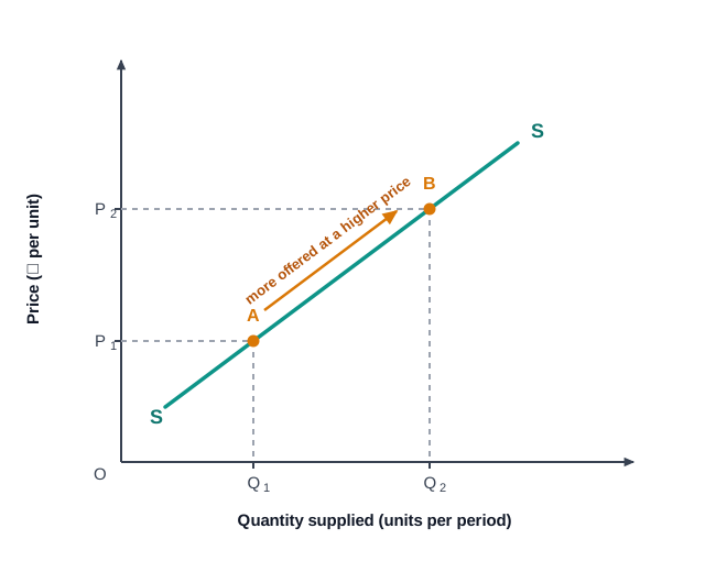
Fig. 5.0 – Sellers offer more at a higher price.

5.1 Concept of Supply

Every market has two sides. The study of demand looked at the buyer, who must spread a limited income over competing wants. This chapter turns to the seller, who faces a choice of the same kind from the other direction. Land, labour, capital and enterprise are scarce and can be put to more than one use, so a producer who makes more of one commodity must make less of something else.

How much of a commodity is placed before buyers is therefore a decision about scarce resources and not a mere willingness to trade. Economics gives that decision the name supply. Supply is never a bare quantity lying in a godown; it is a quantity offered at a stated price for a stated period, and it changes as that price changes.

Definition

Supply Supply refers to the quantity of a commodity that producers are willing to produce and offer for sale at a given price during a given period of time.

Three things in this definition decide whether a statement about supply means anything at all.

Three Features Of Supply

A desired quantity — supply is the amount producers are willing to sell, not the amount they finally succeed in selling. What is actually sold depends on the buyers as well, and may fall short of what was offered.
Always expressed at a price — a quantity carries no meaning in supply until the price at which it is offered is stated. Alter the price and the quantity offered alters with it, which is why supply is always read against a price.
A flow and not a fund — supply is measured over a period of time, as so many units per day, per week or per year. A quantity with no period attached to it is not a supply figure.

This is why the statement that a firm will supply 500 shirts is incomplete. It becomes a supply statement only when it reads that the firm will supply 500 shirts a week at a price of ₹400 a shirt, because only then is the offer tied to a price and to a period.

Watch Out

Supply is the quantity producers are willing to offer for sale. It is not the quantity they actually manage to sell, which depends on the buyers as well.

5.1.1 Individual Supply and Market Supply

A single producing unit is called a firm in economics, and all the firms producing a commodity together make up an industry. Supply can be measured at either level, and the two measures answer different questions.

Individual supply refers to the various quantities of a commodity that one firm is willing to produce and offer for sale at different prices during a specified period. It describes the conduct of a single seller and depends on that seller’s own costs and capacity.

Market supply, also called the industry’s supply, is what buyers as a whole face in the market. It is obtained by adding, at each price, the quantities offered by every firm producing that commodity.

Definition

Market Supply Market supply refers to the total quantity of a commodity that all the producers in the industry are willing to produce and offer for sale at a given price during a given period of time.

Two points follow from this way of adding. First, the summation is carried out price by price, so a market supply figure is meaningless unless the price at which it was arrived at is stated. Second, market supply can change even when no single firm alters its own offer, because the entry of new firms into the industry or the exit of existing ones changes the number of quantities being added.

5.1.2 Stock and Supply

Supply is easily confused with the quantity of a commodity a producer happens to have in hand, and the two must be held apart. Stock is the total amount of the commodity available with the producers or sellers at a given moment. It is what could be offered for sale, and for that reason it is described as potential supply or intended supply.

Supply is that part of the stock which the producers are actually willing to bring into the market and offer for sale at a particular price. It is therefore called actual supply. A trader who buys foodgrains from farmers immediately after the harvest holds a large stock; the quantity he is willing to release into the market this month at the ruling price is his supply, and it is only a fraction of what lies in his warehouse.

The sharpest difference between the two lies in their time dimension. Stock is measured at a point of time — the stock of foodgrains with a trader on 1 April. Supply is measured over a period of time — the supply of foodgrains during the month of April. Stock is also the ceiling on supply, since a seller cannot offer more than he holds, and how tightly that ceiling binds depends on how quickly fresh output can be produced. The relation between the two is shown in Fig. 5.1.

Fig. 5.1

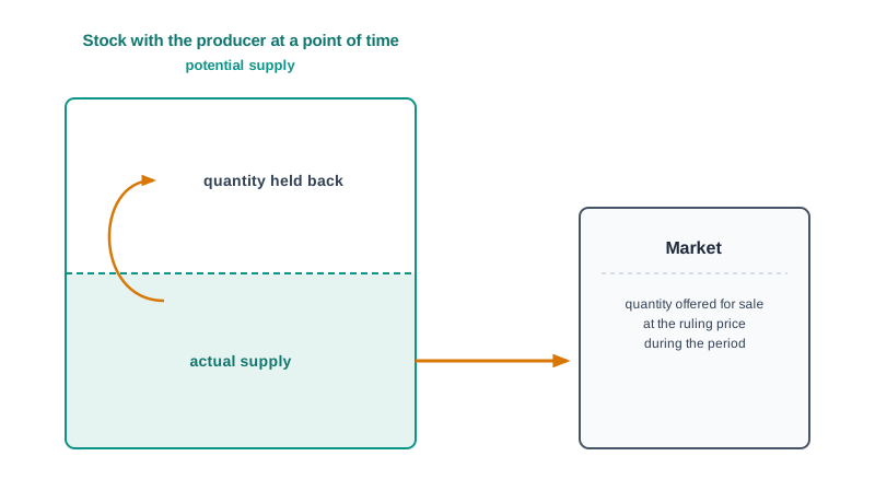
Fig. 5.1 – Stock and supply.

Economy Example

Wheat In The Godowns Of The Food Corporation Of India The Food Corporation of India holds buffer stocks of wheat and rice in its godowns. The quantity lying there on a given date is stock, not supply. Supply is the quantity the Corporation releases to buyers under the Open Market Sale Scheme at an announced price over a stated period. The remainder stays in the godowns as potential supply.

The main points of difference are set out below.

Compare Table

Exam Pointer

ISC repeatedly asks you to distinguish intended supply from actual supply. Answer it as the stock and supply distinction, and state the time dimension of each — stock at a point of time, supply over a period. Marks are lost when that contrast is left out.

5.2 Determinants of Supply

A producer deciding how much to offer for sale is weighing what the output will fetch against what it will cost to make. Anything that alters either side of that comparison alters the quantity offered. The price of the commodity is only the first of these influences, and a theory built on price alone would leave most of a producer’s conduct unexplained.

The factors listed below are the determinants of supply. They are set out separately here because the law of supply, taken up in the next section, deliberately isolates one of them — the commodity’s own price — and holds the rest constant. Knowing what is being held constant is what makes that law usable, and it is also what tells us, later in the chapter, why the whole supply curve sometimes moves.

Factors On Which Supply Depends

Price of the commodity — the most important determinant of supply is the commodity’s own price. Given the cost per unit, a higher price widens the profit on each unit sold, which induces existing firms to produce more and draws new firms into the industry.
Prices of the factors of production — the prices of raw materials, labour, power and machinery decide the cost of production. A rise in input prices narrows the profit margin at any given price of the commodity, so less is produced and offered; a fall in input prices has the opposite effect. Supply therefore moves in the direction opposite to input prices.
Prices of related commodities — here the relation is one of production rather than consumption. A farmer whose land can carry either peas or cabbage will divert land to peas when the price of peas rises, and the supply of cabbage will fall even though nothing has happened to the price of cabbage.
Technique of production — an improved technique, a new machine or a better process lowers the cost of producing each unit and raises the profit earned on it. More is then produced at every price, which is why technical progress is among the strongest causes of an increase in supply.
Goals of the firm — economic theory ordinarily assumes that a firm aims at maximum profit, and the determinants above are read in that light. A firm aiming instead at maximum sales, for the standing it brings in the market, will produce more than the profit-maximising output, while a firm anxious to keep risks small will produce less.
Number of firms in the industry — market supply is the sum of what individual firms offer, so it depends on how many firms there are. Entry of new firms raises market supply at every price and exit lowers it, even if no existing firm changes its own offer.
Structure of the industry — a monopolist, being the only producer, can restrict output in order to hold the price up. Where many firms compete, no single firm gains by holding back, so a competitive industry ordinarily offers more of the commodity than a monopolised one.
Taxes and subsidies — an indirect tax on a commodity adds to the cost the producer must recover and works like a rise in the cost of production, so supply falls. A subsidy works the other way, reducing the effective cost and inducing producers to offer more.
Expectations about future prices — a producer who expects the price to rise shortly will hold back part of the present output in order to sell it later on better terms, and current supply falls. An expected fall in price has the reverse effect, as sellers hurry to clear their stocks now.
Natural factors — the supply of agricultural commodities depends heavily on rainfall, temperature and the absence of pests and floods. A failed monsoon or unseasonal rain reduces the harvest and therefore the quantity that can be offered, whatever the price may be.
Agreement among producers — producers sometimes act together and agree to restrict the quantity placed on the market so as to keep the price high. Such an agreement creates an artificial scarcity, and supply falls without any change in cost or in technique.

Watch Out

Prices of related commodities here means goods the producer could make instead, not goods the buyer could buy instead. The substitution is in production, not in consumption.

Economy Example

Incentives And The Supply Of Electronics Under the Production Linked Incentive schemes announced from 2020, the Government of India pays manufacturers an incentive linked to their additional output of goods made in India, including mobile phones and other electronics. The incentive lowers the effective cost of producing each extra unit, and firms respond by expanding capacity and offering a larger quantity at the same price.

Exam Pointer

A question asking what shifts the supply curve wants factors other than the commodity’s own price. Listing the own price among them earns no mark, because a change in own price moves the seller along the curve rather than shifting it.

5.2.1 The Supply Function

Listing the determinants one by one shows what supply depends on but not how they act together. The supply function states the whole relationship compactly: it says that the quantity supplied of a commodity is determined by its own price and by the other determinants taken together, without yet saying which way each one pulls.

Definition

Supply Function A supply function is a statement of the relationship between the quantity supplied of a commodity and all the factors that determine it.

For a commodity \(x\), the supply function may be written as follows.

\[S_x = f(P_x,\ P_1 \ldots P_n,\ F_1 \ldots F_m,\ T,\ G_f,\ G_t,\ E,\ N)\]

Here \(S_x\) is the quantity supplied of commodity \(x\), measured in physical units per period; \(f\) shows that the quantity supplied depends on the terms that follow; \(P_x\) is the price of commodity \(x\) in ₹ per unit; \(P_1 \ldots P_n\) are the prices of other commodities; \(F_1 \ldots F_m\) are the prices of the factors of production; \(T\) is the technique of production; \(G_f\) is the goal of the firm; \(G_t\) is the taxation and subsidy policy of the government; \(E\) is the expectation about future prices; and \(N\) stands for natural factors. The equation is read as a list of everything the quantity offered responds to, not as a formula to be solved for a number.

A relationship with nine determinants cannot be drawn or reasoned about all at once, so economics takes it one variable at a time. Allowing the own price to vary and holding every other determinant constant — the assumption of ceteris paribus — reduces the function to its simplest form.

\[S_x = f(P_x)\]

In this form \(S_x\) is again the quantity supplied per period and \(P_x\) the own price in ₹ per unit, and every other determinant is treated as fixed. Read this way, the function says that the quantity offered varies with the commodity’s own price alone, which is exactly the statement the law of supply goes on to make precise.

5.3 The Law of Supply

The supply function says that the quantity offered depends on the own price along with much else. To build a usable theory of price, economics needs something sharper: a statement of which way the quantity offered moves when the own price moves and everything else is held still. That statement is the law of supply.

The law rests on the producer’s arithmetic. At a given cost per unit, a higher price leaves a larger margin on every unit sold, and the prospect of that margin is what draws out a larger quantity. The direction of the relationship is therefore positive, unlike the law of demand, where price and quantity move in opposite directions.

Definition

Law of Supply Other things remaining the same, the quantity of a commodity that producers are willing to produce and offer for sale rises with a rise in its price and falls with a fall in its price.

The phrase ‘other things remaining the same’ is not a formality. It is the ceteris paribus assumption, and it names precisely what must stay fixed for the law to hold.

Assumptions Of The Law Of Supply

Prices of the factors of production remain unchanged, so that the cost of producing each unit does not move while the price of the commodity moves.
The technique of production remains unchanged, since a new technique would alter cost independently of price.
Prices of related commodities remain unchanged, so that the producer has no fresh reason to divert resources to some other product.
The taxation and subsidy policy of the government remains unchanged.
The goals of the firms, the number of firms in the industry and natural conditions remain unchanged.

Exam Pointer

State the law in full — ‘other things remaining the same’ and both directions of the change. An answer that gives only the rise and omits the qualifying phrase or the fall does not earn the definition mark.

The law can be shown in two ways, by a supply schedule and by a supply curve. They carry the same information; one presents it in figures and the other in a picture.

5.3.1 Supply Schedule

A supply schedule sets out, in a table, the quantity a seller is willing to offer at each of several prices during a given period. It is drawn up on the same assumption as the law itself, that nothing but the own price is allowed to change.

Definition

Supply Schedule A supply schedule is a tabular statement showing the various quantities of a commodity that producers are willing to produce and offer for sale at various alternative prices during a given period of time.

A supply schedule is of two kinds. An individual supply schedule shows the quantities offered by a single firm, and a market supply schedule shows the quantities offered by all the firms in the industry taken together. Table 5.1 gives the individual supply schedule of a firm making notebooks.

Table

Table 5.1 — Individual Supply Schedule Of Firm P For Notebooks | Price (₹ per notebook) | Quantity supplied by Firm P (notebooks per month) | Point on the supply curve | |—|—|—| | 20 | 100 | A | | 25 | 150 | B | | 30 | 200 | C | | 35 | 250 | D | | 40 | 300 | E |

The schedule is read one row at a time. At ₹20 the firm is willing to offer 100 notebooks a month; at ₹30 it is willing to offer 200. Every rise in price is met by a larger quantity offered, which is the law of supply expressed in figures. The table says nothing about how many notebooks the firm will actually sell, since that depends on the buyers.

Suppose the industry consists of only two firms, P and Q. The market supply at each price is then obtained by adding what the two of them offer at that price, as in Table 5.2.

Table

Table 5.2 — Market Supply Schedule For Notebooks | Price (₹ per notebook) | Supplied by Firm P (notebooks per month) | Supplied by Firm Q (notebooks per month) | Market supply (Firm P + Firm Q) | |—|—|—|—| | 20 | 100 | 60 | 160 | | 25 | 150 | 90 | 240 | | 30 | 200 | 120 | 320 | | 35 | 250 | 150 | 400 | | 40 | 300 | 180 | 480 |

Two things are worth noticing in Table 5.2. The addition is carried out across a row and never down a column, because only quantities offered at the same price may be added. And market supply obeys the law of supply for the same reason each firm does, since a sum of rising quantities must itself rise.

5.3.2 Supply Curve

The same information can be presented graphically. Price is measured on the vertical axis and quantity supplied on the horizontal axis, each price–quantity pair of the schedule is plotted as a point, and a smooth line is drawn through the points.

Definition

Supply Curve A supply curve is a curve showing the various quantities of a commodity that producers are willing to produce and offer for sale at different prices during a given period of time, other things remaining the same.

Like the schedule, the curve is of two kinds, individual and market. It slopes upward from left to right, and that positive slope is simply the law of supply drawn as a picture: a higher point on the price axis is matched by a point further to the right on the quantity axis. The curve may be a straight line or a curved line; what matters for the law is the direction of the slope and not its shape.

Two features of the curve repay attention. First, it begins at a definite price and not at the origin. In Table 5.1 the firm offers nothing below ₹20, so the curve starts at point A. The price below which a seller is not willing to part with any quantity is called the reserve price. Second, the whole curve is drawn for one set of other determinants; change any of them and a different curve must be drawn, a point taken up in Section 5.4. The individual supply curves of the two firms and the market supply curve derived from them are shown together in Fig. 5.2.

Fig. 5.2

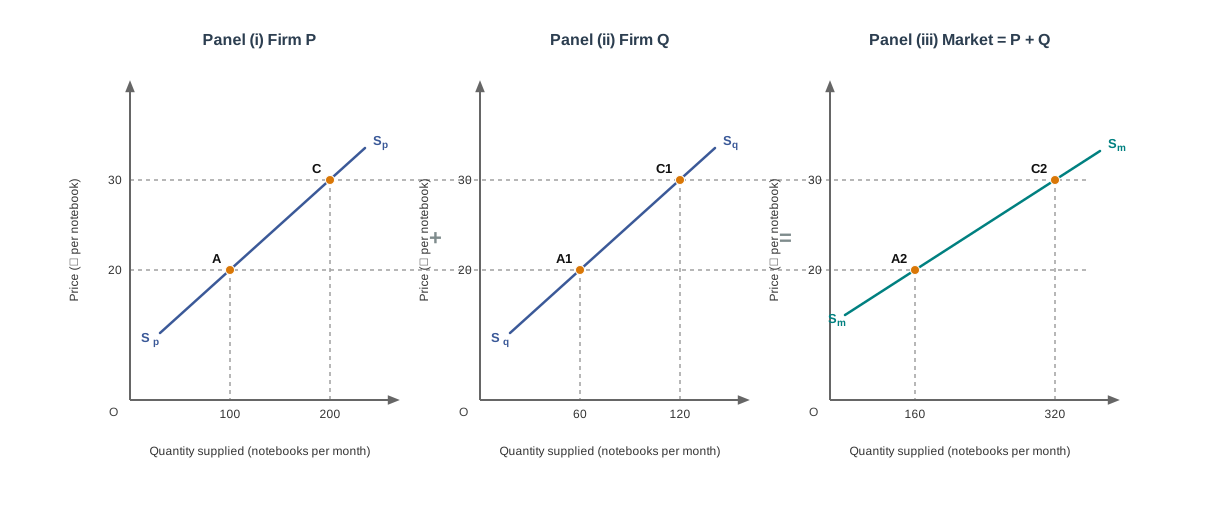
Fig. 5.2 – Derivation of the market supply curve.

5.3.3 Derivation of the Market Supply Curve

Panel (iii) of Fig. 5.2 was obtained by plotting the market supply schedule directly, but it can also be built up from the individual curves themselves. Since quantity is measured along the horizontal axis, the two individual curves are added horizontally, price by price.

The procedure is read off the figure as follows. At the price of ₹20, Firm P offers the quantity shown by point A in Panel (i) and Firm Q offers the quantity shown by point A1 in Panel (ii). Adding the two horizontally gives point A2 in Panel (iii). Repeating this at ₹30 gives point C2 from points C and C1, and repeating it at every other price gives every other point on SmSm. Joining these points yields the market supply curve, which is why the market curve is also called the industry’s supply curve.

Two consequences follow. The market curve is flatter than either individual curve, because the same rise in price now draws out the response of both firms together. And the market curve shifts whenever the number of firms changes, since a curve is being added to or removed from the summation even though no existing firm has altered its own offer.

5.3.4 Why the Supply Curve Slopes Upward

The upward slope is a conclusion and not an assumption, and three separate forces produce it.

Profit at the margin — with the cost per unit given, a higher price widens the profit earned on each unit sold. The price acts as an incentive, and the stronger the incentive the more a producer is willing to place on the market, ceteris paribus.
Rising marginal cost — as a firm expands output with a plant of a given size, the cost of producing each additional unit ordinarily rises, for reasons studied under the law of variable proportions. A producer will therefore go on adding units only if the price rises far enough to cover the higher cost of the last unit produced.
Entry of new producers — a higher price attracts firms that were not producing the commodity at all, since resources can now be moved into it profitably from elsewhere. Market supply rises both because existing firms produce more and because there are more firms producing.

Watch Out

The law of supply tells us how the quantity offered responds to a price. It does not say that a seller can fix the price; that is settled by demand and supply together.

5.3.5 Time Period and Supply

How far supply can respond to a price depends on how much time the producer has, because a response means producing, and production cannot be hurried past a point. Economists therefore distinguish three periods, illustrated together in Fig. 5.3.

Market period — a period so short that output cannot be altered at all. The maximum that can be offered is the stock already produced, so the supply curve is a vertical straight line and the quantity is the same whatever the price. Vegetables already brought to the market that morning are the standard case.
Short run — a period long enough for output to be varied with the existing plant, by running extra shifts or employing more labour and materials, but not long enough to build new plants. Supply can be increased, though only to a limited extent, so the short-run supply curve is upward sloping but steep.
Long run — a period long enough for firms to build new plants, install new machinery and for new firms to enter the industry. A large change in quantity supplied then becomes possible, so the long-run supply curve is upward sloping and comparatively flat.

Fig. 5.3

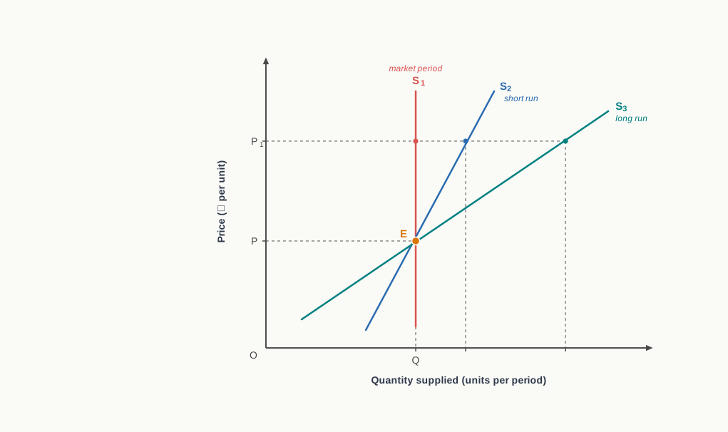
Fig. 5.3 – Supply curves and the time period.

Economy Example

Sugar And The Crushing Season Sugar mills in Uttar Pradesh and Maharashtra crush the cane standing in the fields of that season. Once the cane has been planted, a rise in the price of sugar cannot bring out much more sugar within the season, because the raw material is already fixed. A larger output has to wait for the next planting, which is a short-run limit turning into a long-run response.

5.3.6 Exceptions to the Law of Supply

The law of supply holds in the great majority of cases, but not in all. Two exceptions matter, and in both of them a higher price fails to bring out a larger quantity.

Fixed supply — the supply of some commodities cannot be increased at all, however high the price goes. Rare coins, old manuscripts and original paintings are of this kind, and their supply curve is a vertical straight line like S1S1 in Fig. 5.3. The same shape appears temporarily whenever a crop has already been harvested, since the season’s output cannot be added to.
Backward sloping supply curve of labour — labour is supplied by a worker in the form of hours of work, and its price is the wage rate. As the wage rises the worker at first offers more hours, preferring work to leisure because each hour now earns more. Beyond a certain wage he has enough income and begins to value leisure more highly, so a further rise in the wage draws out fewer hours, not more. The curve bends backward, as in Fig. 5.4.

Fig. 5.4

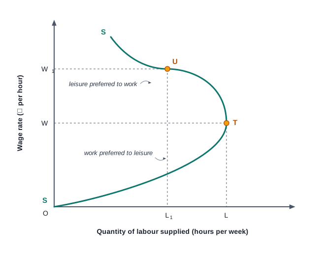
Fig. 5.4 – Backward sloping supply curve of labour.

5.4 Movement Along and Shift of the Supply Curve

A supply curve is drawn for one price at a time but for one set of everything else. That is the source of a distinction which runs through the whole of price theory. When the commodity’s own price changes, the seller moves to a different point on the same curve. When any other determinant changes, the curve itself has to be redrawn.

Both events raise or lower the quantity offered, so they are easy to confuse. They are kept apart by asking a single question: what changed? If the answer is the own price, the change is a movement along the curve. If the answer is anything else, the change is a shift of the curve.

5.4.1 Expansion and Contraction of Supply

When the quantity offered alters because the commodity’s own price has altered, other factors remaining the same, the alteration is called a change in quantity supplied. It is shown by moving from one point to another on a given supply curve.

Definition

Change in Quantity Supplied A change in quantity supplied is a rise or fall in the quantity offered for sale brought about by a change in the commodity’s own price, other factors affecting supply remaining the same.

A movement in the two directions carries two names. A rise in the quantity offered following a rise in the own price is called an expansion of supply, also described as an extension or an upward movement along the curve. A fall in the quantity offered following a fall in the own price is called a contraction of supply, a downward movement along the same curve. Both are illustrated in Fig. 5.5.

Fig. 5.5

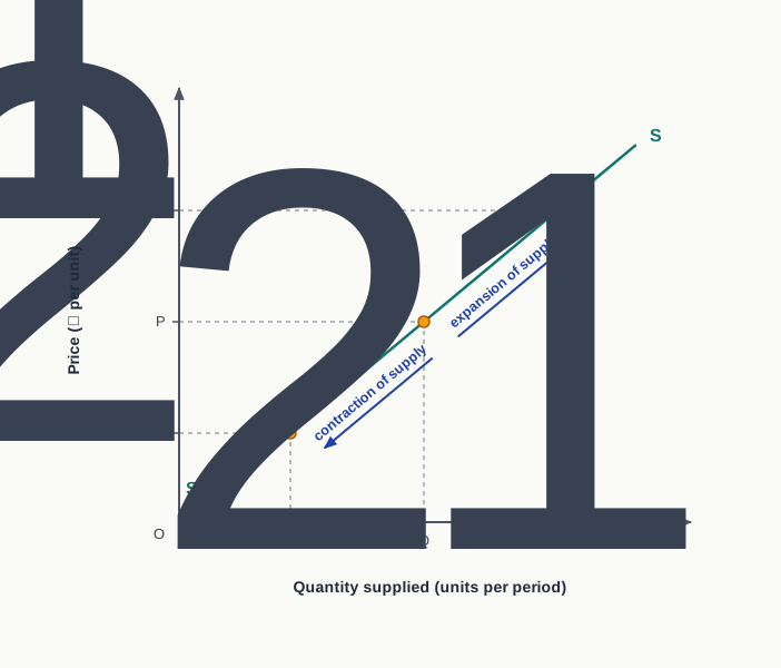
Fig. 5.5 – Expansion and contraction of supply.

Read the figure from point A. When the price rises from OP to OP1 the seller moves up the curve to B and the quantity offered rises from OQ to OQ1; when the price falls from OP to OP2 the seller moves down to C and the quantity offered falls from OQ to OQ2. In both movements the curve SS has stayed exactly where it was, because nothing except the own price has changed.

5.4.2 Increase and Decrease in Supply

The quantity offered may also change while the price stands still. A fall in input prices, an improved technique or a production subsidy makes the same output cheaper to produce, and the producer is then willing to offer more of the commodity at the very same price. Such a change is called a change in supply, and it is shown by shifting the entire curve.

Definition

Change in Supply A change in supply is a rise or fall in the quantity offered for sale at each price, brought about by a change in factors other than the commodity’s own price.

An increase in supply means that producers are willing to offer a larger quantity at the same price, or the same quantity at a lower price. The whole curve moves to the right. A decrease in supply means that producers are willing to offer a smaller quantity at the same price, or the same quantity only at a higher price. The whole curve moves to the left. Fig. 5.6 shows both.

Fig. 5.6

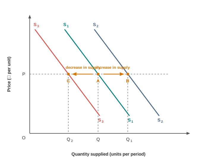
Fig. 5.6 – Increase and decrease in supply.

The price line at OP is the heart of the diagram. It is held fixed so that the movement from A to B, and from A to C, can be attributed to something other than price. The factors that produce these shifts are the determinants of Section 5.2, and their direction of working is collected in Table 5.3.

Table

Economy Example

Minimum Support Price And What Farmers Sow When the Government of India raises the minimum support price of paddy, the higher price for paddy itself draws out a larger quantity of paddy — a movement along its own supply curve. For crops competing with paddy for the same land and water, however, nothing has happened to their own price. Land is diverted away from them, and their supply curves shift to the left.

Watch Out

An increase in supply is not the same as an increase in the quantity supplied. The first shifts the whole curve; the second is a movement along a curve that has not moved.

5.4.3 Change in Quantity Supplied and Change in Supply

The two changes can now be set against each other. The test is always the cause, never the size of the change: a large expansion is still a movement along the curve, and a small increase is still a shift of it.

Compare Table

The pair most often confused is an expansion of supply with an increase in supply, since both leave a larger quantity on the market. They are compared below and drawn side by side in Fig. 5.7.

Compare Table

Fig. 5.7

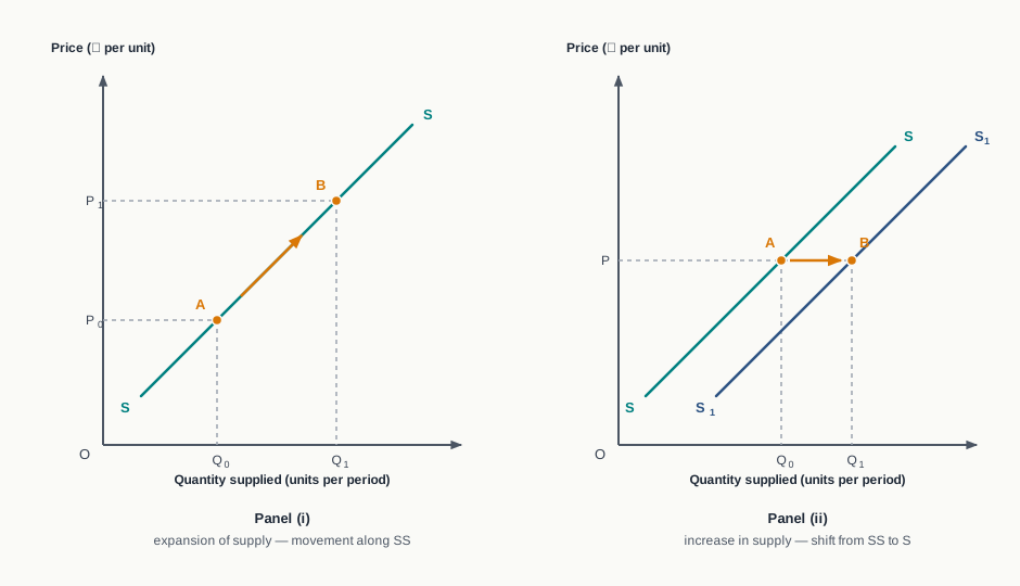
Fig. 5.7 – Expansion versus increase in supply.

The mirror image of each holds without further argument. A contraction of supply is a downward movement along an unchanged curve caused by a fall in the own price, while a decrease in supply is a leftward shift of the whole curve caused by something else, such as a rise in input prices or a withdrawal of a subsidy. In every case the question to ask first is which variable moved.

Exam Pointer

When you draw a shift, mark the unchanged price on the vertical axis and drop verticals to both quantities. An unlabelled shift diagram does not show what has been held constant, and the mark is given for showing it.

5.5 Elasticity of Supply

The law of supply tells us the direction in which the quantity offered will move when the price moves. It does not tell us by how much. Yet the size of the response is what matters in practice, since a price rise that brings out a flood of extra output has very different consequences from one that brings out a trickle.

The problem is one of measurement, and units complicate it. Supply may be counted in kilograms, litres, metres or dozens, and price in rupees per kilogram or rupees per dozen, so a comparison of absolute changes would depend on the units chosen. The tool economics uses gets round this by comparing proportionate changes, which are pure numbers.

5.5.1 Meaning of Elasticity of Supply

Elasticity of supply measures how sensitive the quantity offered is to a change in the commodity’s own price. It answers the question by how much rather than in which direction, and because it compares one proportionate change with another, its answer holds whatever the units of measurement may be.

Definition

Elasticity of Supply Price elasticity of supply is the degree of responsiveness of the quantity supplied of a commodity to a change in its price. It is the proportionate change in quantity supplied divided by the proportionate change in price.

Elasticity of supply carries a positive sign. Price and quantity supplied move in the same direction under the law of supply, so the two proportionate changes are either both positive or both negative and their ratio is positive. This is a real difference from elasticity of demand, where the ratio is negative and the sign is dropped by convention before the answer is read.

5.5.2 Degrees of Elasticity of Supply

The numerical value of elasticity of supply can lie anywhere between zero and infinity, and five values or ranges are given names. All five are drawn together in Fig. 5.8.

Perfectly elastic supply — sellers are willing to offer any quantity whatever at the ruling price, but nothing at all at a price even slightly lower. The supply curve is a horizontal straight line and elasticity is infinite. It is an extreme case, useful as a benchmark rather than as a description of any real market.
Perfectly inelastic supply — the quantity offered stays the same however much the price changes, so elasticity is zero and the supply curve is a vertical straight line. The supply of a commodity in the market period, and of goods that cannot be reproduced at all, is of this kind.
Unitary elastic supply — the percentage change in quantity supplied is exactly equal to the percentage change in price, so elasticity is one. Any straight line supply curve drawn through the origin has unit elasticity over its entire length, whatever its slope.
Elastic supply — the percentage change in quantity supplied is greater than the percentage change in price, so elasticity is greater than one. Any straight line supply curve that cuts the Y-axis is elastic throughout, though the exact value differs from point to point.
Inelastic supply — the percentage change in quantity supplied is less than the percentage change in price, so elasticity lies between zero and one. Any straight line supply curve that cuts the X-axis is inelastic throughout.

Fig. 5.8

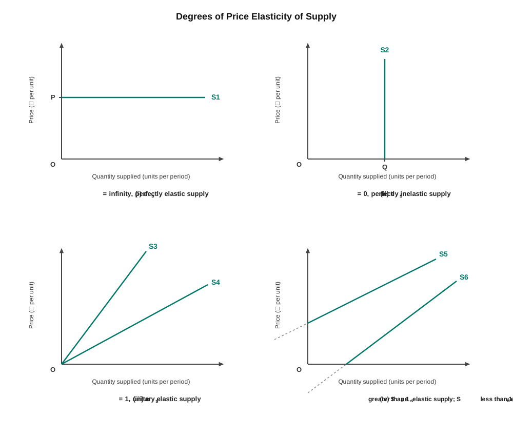
Fig. 5.8 – Degrees of elasticity of supply.

The five cases and the shapes that go with them are collected in Table 5.4, which is worth committing to memory, since a question often gives the shape and asks for the degree, or gives the degree and asks for the shape.

Table

Watch Out

A steeper curve is not automatically the less elastic one. Every straight line drawn through the origin has unit elasticity, however steep or flat it happens to be.

5.5.3 Measurement of Elasticity of Supply

Elasticity of supply can be measured in two ways. The percentage method computes it from two price and quantity pairs, while the geometric or point method reads it off the supply curve at a single point.

5.5.3.1 Percentage Method

The percentage method applies the definition directly, dividing the proportionate change in quantity supplied by the proportionate change in price. Both are taken on the original values, so that the base of the calculation is fixed before anything moves.

\[e_s = \dfrac{\Delta Q / Q}{\Delta P / P} = \dfrac{\Delta Q}{\Delta P} \times \dfrac{P}{Q}\]

Here \(e_s\) is the elasticity of supply, \(\Delta Q\) the change in quantity supplied and \(Q\) the original quantity, both in physical units; \(\Delta P\) is the change in price and \(P\) the original price, both in ₹ per unit. The result is a pure number with no unit. A value above one means supply is elastic, below one inelastic, and exactly one unitary elastic.

Example 5.1

Elasticity Of Supply By The Percentage Method

The price of a commodity rises from ₹25 to ₹30 per unit, and the quantity supplied rises from 400 units to 520 units. Calculate the elasticity of supply and state the degree of elasticity.

\(\Delta Q = 520 - 400 = 120\) units

\(\Delta P = 30 - 25 = ₹5\)

\(Q = 400\) units, \(P = ₹25\)

\(e_s = \dfrac{\Delta Q}{\Delta P} \times \dfrac{P}{Q} = \dfrac{120}{5} \times \dfrac{25}{400}\)

\(e_s = 24 \times 0.0625 = 1.5\)

Since \(e_s > 1\), the supply of the commodity is elastic.

The same formula answers the reverse question, in which the elasticity is given and a quantity or a price is to be found. The working is simply rearranged, as in SE 5.2.

Example 5.2

Finding The Quantity Supplied At A New Price

A producer supplies 800 units of a commodity at ₹40 per unit. The elasticity of supply is 2. How many units will the producer supply at ₹44 per unit?

\(P = ₹40\), \(Q = 800\) units, \(\Delta P = 44 - 40 = ₹4\), \(e_s = 2\)

\(e_s = \dfrac{\Delta Q}{\Delta P} \times \dfrac{P}{Q}\)

\(2 = \dfrac{\Delta Q}{4} \times \dfrac{40}{800}\)

\(2 = \dfrac{\Delta Q}{80}\)

\(\Delta Q = 2 \times 80 = 160\) units

New quantity supplied \(= 800 + 160 = 960\) units

The producer will supply 960 units at ₹44 per unit.

Exam Pointer

Substitute the original price and the original quantity, never the new ones, and set out \(\Delta Q\), \(\Delta P\), \(Q\) and \(P\) before the formula. Finish by naming the degree, since a bare number is an incomplete answer.

5.5.3.2 Geometric Method

The percentage method needs two price and quantity pairs. The geometric method needs only one point on the curve, which is why it is also called the point method.

Take a point K on a straight line supply curve, at which the quantity supplied is OB. Extend the curve downward until it meets the X-axis at A. Elasticity at K is then the ratio of the horizontal segment AB to the quantity OB.

\[e_s = \dfrac{AB}{OB}\]

Here AB is the distance along the X-axis between the point at which the supply curve meets that axis and the foot of the perpendicular dropped from K, while OB is the quantity supplied at K, both measured in the units of the horizontal axis. The ratio is a pure number and is read exactly as before. The three possible cases are shown in Fig. 5.9.

Fig. 5.9

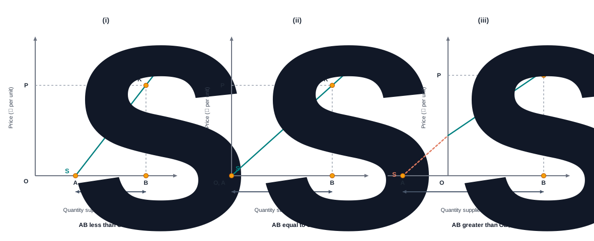
Fig. 5.9 – Geometric measurement of elasticity.

Three rules follow at once and are worth stating separately. A straight line supply curve that cuts the X-axis has elasticity less than one throughout. One that passes through the origin has elasticity exactly equal to one at every point on it. One that cuts the Y-axis has elasticity greater than one throughout.

On a curved supply line the slope differs at every point, so elasticity must be measured point by point. A tangent is drawn to the curve at the chosen point and extended to meet the X-axis, and the same ratio is then applied to that tangent, as in Fig. 5.10.

Fig. 5.10

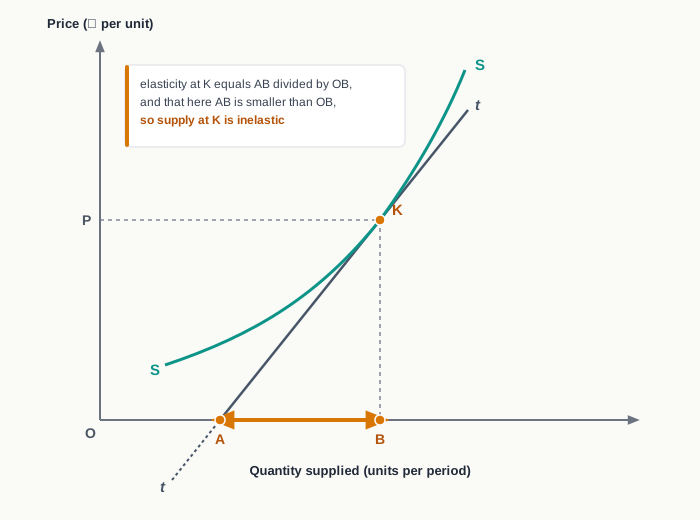
Fig. 5.10 – Elasticity on a non-linear supply curve.

5.5.4 Determinants of Elasticity of Supply

Whether supply is elastic or inelastic is not a matter of chance. It depends on how easily and how quickly a producer can expand output, which is a question about resources and about time.

Time period — this is the most powerful influence of all. In the market period output cannot be changed and supply is perfectly inelastic; in the short run it can be varied within the existing plant, so supply is inelastic but no longer fixed; in the long run new plants can be built and new firms can enter, so supply becomes elastic.
Behaviour of cost — if producing additional units raises the cost per unit only slightly, a small rise in price is enough to make the extra output worth producing and supply is elastic. If cost climbs steeply as output expands, the same price rise draws out very little and supply is inelastic.
Nature of the commodity — durable goods can be stored, so producers can add to the market from stocks or withhold from them, and their supply is relatively elastic. Perishable goods cannot be stored, so any change in what is offered must come out of current production, which makes their supply relatively inelastic.
Availability of spare capacity — a firm with idle machinery, spare labour and assured power can raise output quickly when the price rises. Where plants already run at their limit, or power and raw materials are short, output expands slowly and supply is inelastic.
Nature of the inputs — a commodity made with inputs that are freely available can be produced in larger quantity at short notice. One that needs a specialised input, such as a rare skill or a scarce raw material, has an inelastic supply.
Complexity of the technique — where production involves a long and complicated process, output cannot be raised quickly and supply is inelastic. Simple processes that can be repeated easily give an elastic supply.
Mobility of the factors of production — the more easily land, labour and capital can be shifted out of other uses into the production of this commodity, the larger the response to a price rise. Immobile factors make supply inelastic.
Willingness to bear risk — expanding output commits a producer to expenditure before the return is known. Entrepreneurs willing to carry that risk make supply more elastic, and cautious entrepreneurs make it less so.

Economy Example

Why Housing Supply Responds Slowly When flat prices rise sharply in a large Indian city, the number of flats available does not rise with them for several years. Land within the city is fixed, and building needs approvals, finance and construction time. Supply is close to perfectly inelastic in the short run, and becomes elastic only over a period long enough for new projects to be completed.

5.6 Summary

Supply refers to the quantity of a commodity that producers are willing to produce and offer for sale at a given price during a given period of time. Three features are essential to the idea:
1. It is a desired quantity, not the quantity actually sold.
2. It is always stated with reference to a price.
3. It is a flow, measured over a period of time.
Individual supply is the quantity a single firm is willing to offer at a given price, while market or industry supply is the total offered by all the firms in the industry, obtained by adding the individual quantities price by price.
Stock is the total quantity available with the seller at a point of time and is potential or intended supply; supply is that part of the stock actually offered for sale over a period at a given price, and is actual supply. Stock sets the ceiling on supply.
The determinants of supply are:
1. Price of the commodity
2. Prices of the factors of production
3. Prices of related commodities
4. Technique of production
5. Goals of the firm
6. Number of firms in the industry
7. Structure of the industry
8. Taxes and subsidies
9. Expectations about future prices
10. Natural factors
11. Agreement among producers
The supply function collects these determinants into one statement, \(S_x = f(P_x,\ P_1 \ldots P_n,\ F_1 \ldots F_m,\ T,\ G_f,\ G_t,\ E,\ N)\), where \(S_x\) is the quantity supplied of commodity \(x\) in units per period, \(P_x\) its own price in ₹ per unit, \(P_1 \ldots P_n\) the prices of other commodities, \(F_1 \ldots F_m\) the prices of the factors of production, \(T\) the technique of production, \(G_f\) the goal of the firm, \(G_t\) the taxation and subsidy policy, \(E\) expectations about future prices and \(N\) natural factors.
Holding every determinant except the own price constant reduces the function to \(S_x = f(P_x)\), the form in which the law of supply is stated.
The law of supply states that, other things remaining the same, the quantity of a commodity that producers are willing to offer for sale rises with a rise in its price and falls with a fall in its price. It assumes no change in input prices, technique, prices of related commodities, government policy, the goals of firms, the number of firms or natural conditions.
A supply schedule is a tabular statement of the quantities offered at various prices during a given period, and is of two kinds, individual and market.
A supply curve is the same relationship drawn as a picture, with price on the vertical axis and quantity supplied on the horizontal axis. It slopes upward from left to right and begins at the reserve price, the price below which a seller offers nothing.
The market supply curve is derived by adding the individual supply curves horizontally at each price. It is flatter than any individual curve and shifts when the number of firms in the industry changes.
The supply curve slopes upward for three reasons:

A higher price widens the profit earned on each unit sold.
Marginal cost rises as output expands, so a higher price is needed to cover the cost of the last unit.
A higher price attracts new firms into the industry.

Supply responds differently over different lengths of time:

Market period — output cannot be varied at all and the supply curve is vertical.
Short run — output can be varied within the existing plant and the supply curve is upward sloping but steep.
Long run — new plants can be built and new firms can enter, so the supply curve is upward sloping and flat.

There are two exceptions to the law of supply:

Fixed supply, as of rare coins or a harvested crop, where the curve is vertical.
The backward sloping supply curve of labour, where beyond a certain wage the worker offers fewer hours because leisure is now preferred to work.

A change in quantity supplied is caused by a change in the commodity’s own price and is shown by a movement along the same supply curve. A rise is called expansion of supply and a fall contraction of supply.
A change in supply is caused by a change in any determinant other than the own price and is shown by a shift of the whole curve. A rightward shift is an increase in supply and a leftward shift a decrease in supply.
Price elasticity of supply measures the degree of responsiveness of the quantity supplied to a change in price. It is \(e_s = \dfrac{\Delta Q / Q}{\Delta P / P} = \dfrac{\Delta Q}{\Delta P} \times \dfrac{P}{Q}\), where \(\Delta Q\) is the change in quantity supplied, \(Q\) the original quantity in units, \(\Delta P\) the change in price and \(P\) the original price in ₹ per unit. The answer is a pure number and is always positive.
There are five degrees of elasticity of supply:

Perfectly elastic, elasticity infinite, curve horizontal.
Perfectly inelastic, elasticity zero, curve vertical.
Unitary elastic, elasticity equal to one, any straight line through the origin.
Elastic, elasticity greater than one, any straight line cutting the Y-axis.
Inelastic, elasticity less than one, any straight line cutting the X-axis.

By the geometric method, elasticity at a point K on the supply curve is \(e_s = \dfrac{AB}{OB}\), where \(AB\) is the distance along the X-axis from the point at which the extended curve or tangent meets that axis to the foot of the perpendicular dropped from K, and \(OB\) is the quantity supplied at K. Elasticity is greater than one when \(AB\) exceeds \(OB\), equal to one when they are equal and less than one when \(AB\) is smaller.
Elasticity of supply depends on the time period allowed, the behaviour of cost as output expands, the durability of the commodity, the availability of spare capacity, the nature of the inputs, the complexity of the technique, the mobility of factors and the producer’s willingness to bear risk.
The four changes in supply distinguished in the chapter are condensed below.

Compare Table

5.7 Points to Ponder

The law of supply holds only when everything other than price stays constant, yet in agriculture the weather, input costs and government policy are changing all the time. Does an assumption that is almost never satisfied still teach a farmer or a policymaker something useful, or does it describe a market that does not exist?
A producer who expects prices to rise and holds back part of his output is behaving exactly as the theory of supply predicts. The same act, when it involves an essential commodity, is called hoarding and is penalised by law. Where would you draw the line between prudent withholding and hoarding, and on what principle?
Beyond a certain wage a worker offers fewer hours, not more, because leisure has become worth more to him than the extra income. What does this say about the common assumption that people always prefer more income to less, and should an economy treat rising leisure as a gain or as a loss of output?
When supply is inelastic in the short run, the whole force of a change in demand falls on the price. Buffer stocks and open market sales can soften that swing, but a price that is not allowed to rise also tells producers nothing about the shortage. Which of the two costs is the greater?
The market supply curve is built by adding individual curves, which assumes that each firm decides on its own. What is left of that curve when the producers act by agreement and fix among themselves how much will reach the market?
A supply curve records only the costs the producer actually pays. If producing more of a commodity also draws down groundwater or fouls a river, the curve understates what the extra output really costs the economy. Should such costs be brought into the producer’s own calculation, and what would happen to supply if they were?

5.8 Objective Questions

A straight line supply curve that cuts the X-axis to the right of the origin has: [1]
1. perfectly elastic supply
2. unitary elastic supply
3. elastic supply
4. inelastic supply
Read the assertion and the reason given below and choose the correct option. [1] Assertion (A): In the market period the supply curve of a perishable commodity is a vertical straight line. Reason (R): In the market period producers cannot alter their output in response to a change in price.
1. Both A and R are true, and R is the correct explanation of A.
2. Both A and R are true, but R is not the correct explanation of A.
3. A is true, but R is false.
4. A is false, but R is true.
Fill in the blank: A leftward shift of the entire supply curve of a commodity is called _______ in supply. [1]
State whether the following statement is true or false: A rise in the price of a commodity shifts its supply curve to the right. [1]
Match the items in Column I with those in Column II. [1]

Column I	Column II
a. A rise in the own price of the commodity	i. Increase in supply
b. A fall in the prices of raw materials	ii. Unitary elasticity of supply
c. A straight line supply curve drawn through the origin	iii. Expansion of supply

5.9 Check Your Concepts

Distinguish between intended supply and actual supply. [2]
The quantity supplied of a commodity at a price of ₹8 per unit is 400 units. The price elasticity of supply is 2. Calculate the price at which the producer will supply 600 units. [3]
Distinguish between expansion of supply and increase in supply, with the help of suitable diagrams. [4]
State the law of supply along with its assumptions, and explain why the supply curve slopes upward from left to right. [6]

5.10 Case-Based Question

Rehan owns a small unit making steel folding chairs. In April he offered 300 chairs a month at a price of ₹900 each. When the price rose to ₹1,000 in May, he offered 380 chairs. In June the price of steel sheet fell sharply, and with the price of chairs still at ₹1,000 he offered 460 chairs.
1. Identify the change that took place in Rehan’s supply between April and May, and the change that took place between May and June, giving a reason for each. [2]
2. Calculate the price elasticity of supply of chairs between April and May, and state its degree. [2]