Chapter 3: Theory of Consumer Behaviour: Marginal Utility and Indifference Curve Analysis
Every consumer meets the same difficulty on entering a market: wants are many, income is fixed, and the prices of goods are given. A household with ₹6,000 a month to spend on groceries cannot buy everything on the shelf. It must decide how much of each item to take home and what to leave behind. Economics treats that decision as a problem of choice under a constraint, and asks a precise question — out of all the bundles a consumer can afford, which one will actually be bought? The answer lies in the satisfaction, or utility, that goods yield. This chapter builds two tools for measuring that satisfaction and for locating the point beyond which no rearrangement of purchases can add to it. The first, cardinal utility analysis, assumes satisfaction can be counted in units. The second, indifference curve analysis, requires only that bundles be ranked. Both explain why a consumer buys more of a good when its price falls, and so supply the reasoning that lies behind the law of demand. The chapter covers utility and its measurement, the law of diminishing marginal utility, the law of equi-marginal utility, indifference curves, the budget line, and consumer’s equilibrium under both approaches.
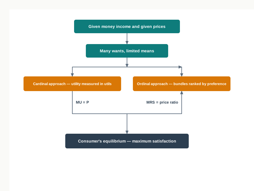
Fig. 3.0 – The consumer’s problem of choice.
3.1 Utility, Total Utility and Marginal Utility
A consumer entering a market carries a fixed income and faces prices that are given. Whatever is spent on one commodity cannot be spent on another, so every purchase is a choice between alternatives. To explain how that choice is made, economics needs a measure of what a commodity is worth to the person buying it.
That measure is utility. The consumer is assumed to be rational, that is, to aim at the largest satisfaction obtainable from a limited income. Before the conditions of such a position can be stated, three ideas have to be kept apart with care: utility itself, the total utility drawn from a given quantity of a commodity, and the utility added by one more unit of it.
3.1.1 Meaning and Characteristics of Utility
A commodity is bought not for its own sake but for the want it satisfies. Bread is bought because it satisfies hunger, a textbook because it meets a want for knowledge, a fan because it makes a hot afternoon bearable. This want-satisfying power is what economics calls utility.
Utility so defined has five features that matter for everything built on it.
- Utility is subjective — it depends on the consumer’s own estimate of the satisfaction a commodity will give, and not on any quality that can be observed in the commodity itself. Two people buying the same good need not derive the same utility from it.
- Utility is not measurable in objective terms — satisfaction is a mental state and cannot be weighed or counted the way length or mass can. Marshall got round this by measuring utility in money, by the amount a consumer is willing to pay for a unit of the commodity. Other economists measure it in imaginary subjective units called utils.
- Utility is relative — it is relative to the intensity of the want, so the same commodity yields different utility to different persons, at different places and at different times. The greater the need, the greater the utility.
- Utility is different from usefulness — a commodity may have utility without being good for the consumer. A cigarette has utility for a smoker because it satisfies a want, although it damages health.
- Utility is devoid of ethical connotations — economics asks only whether a commodity satisfies a want, not whether the want is moral, legal or worth having.
The unit in which utility is measured is called the util. It is an imaginary unit, adopted only so that satisfaction can be handled arithmetically; there is no instrument that reads utils. The approach that treats utility as measurable in such units is called the cardinal approach, and it is the approach followed in the first half of this chapter.
3.1.2 Total Utility and Marginal Utility
A consumer rarely buys a single unit of anything. Satisfaction therefore has to be looked at in two ways: the whole of it, drawn from all the units consumed, and the part of it contributed by the last unit alone. The first is total utility, the second marginal utility.
The difference is best seen in a schedule. Table 3.1 records the utility a consumer obtains from successive cups of tea taken in the course of a day, with the marginal utility of each cup worked out from the total utility column.
The second cup raises total utility from 12 utils to 21 utils, so its marginal utility is 9 utils. The fifth cup leaves total utility unchanged at 30 utils, so it adds nothing and its marginal utility is zero. The sixth cup pulls total utility down from 30 utils to 27 utils, and its marginal utility is therefore negative. When marginal utility is negative, the commodity is said to yield disutility.
Marginal utility is thus the difference between two successive figures of total utility, and this gives the working rule used in every numerical on the topic.
\[MU_n = TU_n - TU_{n-1}\]
Here \(MU_n\) is the marginal utility of the nth unit, \(TU_n\) the total utility from n units and \(TU_{n-1}\) the total utility from one unit less, all three measured in utils. A positive value means the last unit added to satisfaction, zero means it added nothing and a negative value means it reduced satisfaction.
The relation can also be read backwards. Since each unit contributes its own marginal utility, total utility at any level of consumption is nothing but the running sum of those contributions.
\[TU_n = MU_1 + MU_2 + \dots + MU_n = \Sigma MU\]
Here \(TU_n\) is the total utility from n units and \(MU_1\), \(MU_2\) and \(MU_n\) are the marginal utilities of the first, second and nth units, each in utils. In Table 3.1 the total utility of three cups, 27 utils, is exactly \(12 + 9 + 6\).
The two directions of the relationship are set out in SE 3.1 and SE 3.2, which move from a total utility schedule to marginal utility and back again.
3.1.3 Relationship Between Total Utility and Marginal Utility
The two magnitudes move together in a fixed and well-defined order. For the first unit they are equal, since the utility of the first cup of tea in Table 3.1 is at once the whole of total utility and the addition made by that cup. Thereafter they part company, and how they part is the substance of the relationship.
As long as marginal utility is positive, every extra unit adds something and total utility keeps rising. Because marginal utility is itself falling, total utility rises by smaller and smaller amounts, that is, it rises at a diminishing rate. When marginal utility reaches zero, nothing further is being added and total utility stands at its maximum. This is the point of satiety, the point at which the consumer’s desire for that commodity is fully satisfied. Beyond it marginal utility turns negative and total utility begins to fall.
The relationship is shown in Fig. 3.1, where the two curves are drawn one below the other on a common horizontal axis so that each point on the marginal utility curve can be read against the corresponding point on the total utility curve.
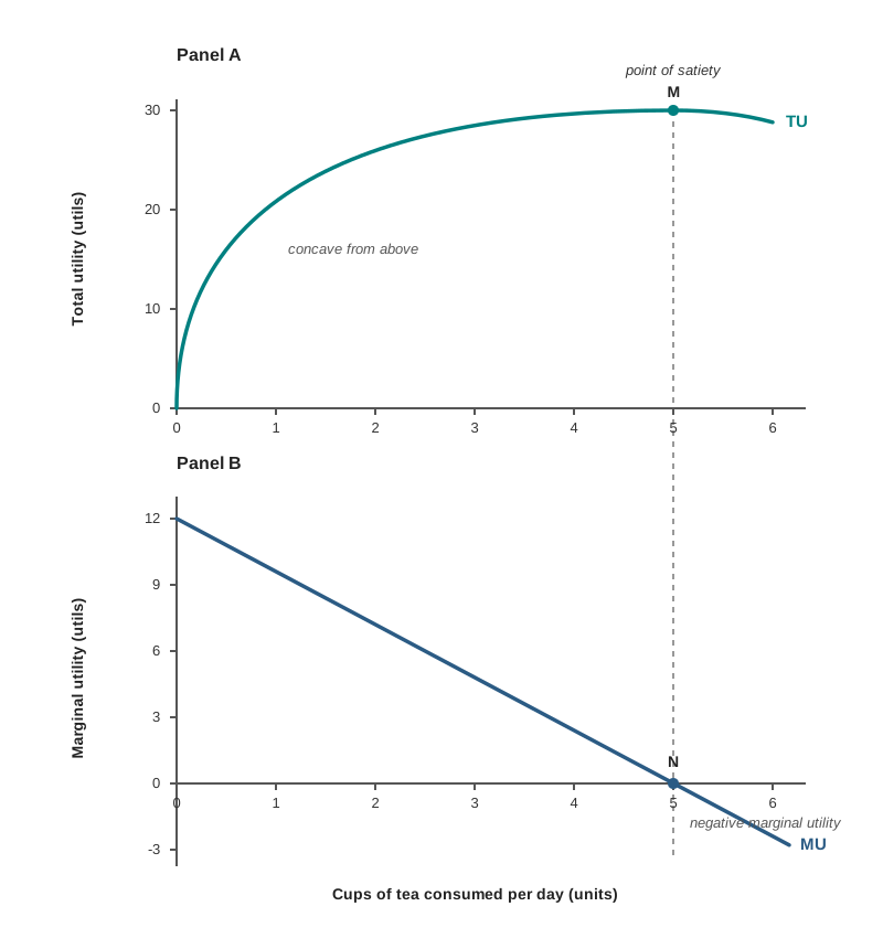
Fig. 3.1 – Total utility and marginal utility curves.
Panel A shows total utility climbing steeply at first, then more gently, reaching its highest point at M and turning downward after it. The flattening of the curve is the diagram’s way of showing marginal utility falling, because the slope of the total utility curve at any quantity is the marginal utility at that quantity. Panel B shows the same information directly: a marginal utility curve sloping downward throughout, cutting the horizontal axis at N and lying below it thereafter.
The relationship can be stated in three propositions, each of which can be read off either the schedule or the diagram.
- Total utility rises so long as marginal utility is positive — the total utility curve slopes upward, but its slope grows steadily smaller, which is why it is concave from above.
- Total utility is at its maximum when marginal utility is zero — at point M the slope of the total utility curve is zero, and the marginal utility curve is passing through N on the horizontal axis.
- Total utility falls when marginal utility is negative — after M the total utility curve slopes downward, and the marginal utility curve lies below the horizontal axis.
Table 3.2 puts the same three positions side by side for quick reference.
A rational consumer will not knowingly buy beyond the point of satiety, since units past that point reduce the very satisfaction being sought. The tendency of marginal utility to fall as consumption grows is so regular that economics states it as a law, and that law is taken up in the next section.
3.2 The Law of Diminishing Marginal Utility
Section 3.1 established that marginal utility falls as consumption grows, and Table 3.1 showed it falling cup by cup. That behaviour is not peculiar to one consumer or to one commodity. It is regular enough for economics to state it as a law, and the whole of utility analysis is built on it.
The law matters because it answers a question a schedule by itself cannot. If every unit yielded the same satisfaction, a consumer would have no reason to stop buying at any particular quantity, and no reason to buy more when the price fell. Diminishing marginal utility supplies both reasons, and with them the explanation of the downward sloping demand curve.
3.2.1 Statement of the Law
The law was first set out by the German economist H. H. Gossen and was given its systematic formulation by Alfred Marshall.
Marshall put the same idea in terms of a stock: the additional benefit a person derives from a given increase in the stock of a thing diminishes with every increase in the stock already held. The qualification ‘other things remaining equal’ belongs to the law and is not an ornament attached to it. It holds income, tastes and the prices of related goods fixed, so that the fall in marginal utility can be attributed to the growing quantity alone.
The law is illustrated in Table 3.3, which records the utility a consumer obtains from chapatis eaten at a single meal.
The first chapati is eaten on an empty stomach and yields 24 utils. Each later one meets a want that has already been partly met, so the addition it makes shrinks steadily: 18 utils, then 12, then 6. The fifth adds nothing and the sixth reduces satisfaction. Total utility meanwhile keeps rising until marginal utility reaches zero, exactly as Section 3.1 showed.
The same fall is shown graphically in Fig. 3.2, where the marginal utility of each unit is drawn as a bar and the curve is passed through the tops of the bars.
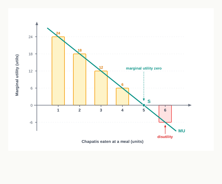
Fig. 3.2 – The law of diminishing marginal utility.
3.2.2 Assumptions of the Law
The law states a tendency that holds only under stated conditions. Each assumption is there to keep out some influence that would otherwise be mistaken for the effect of consuming more.
- All units are identical — the units must be alike in size, colour, design and quality, because a superior later unit could yield more utility than an earlier one and the fall would be interrupted.
- The unit is of a standard size — a cup of water, a full mango, a pair of shoes. A unit that is too small leaves the want largely unmet, so the next unit may add more rather than less.
- Tastes remain unchanged — if the consumer develops a liking for the commodity while consuming it, the marginal utility of a later unit may rise for reasons unconnected with quantity.
- Consumption is continuous — the units must be consumed one after another within a short span, because a long break allows the want to revive and the next unit then yields more.
- Prices of substitutes do not change — a change in the price of a close substitute alters the satisfaction the consumer expects from the commodity itself and makes the comparison unreliable.
- Utility is measurable in cardinal units — the law compares the utility of one unit with that of another, which requires utility to be expressed in numbers, whether in utils or in money.
- The consumer is rational — purchases are made in order to maximise satisfaction, and not out of habit, imitation or compulsion.
- The marginal utility of money is constant — money is the measuring rod here, and a measuring rod that changed length as the consumer spent would make every reading unreliable.
3.2.3 Explanation of the Law
Why should satisfaction behave in this way? Two explanations are usually offered, and they rest on different features of human wants.
- A particular want is satiable — wants taken together are unlimited, but any single want can be satisfied. As more of a commodity is consumed the intensity of that want falls, and with it the satisfaction obtained from each further unit. A hungry person values the first chapati highly because the hunger is sharp; by the fourth, most of it has gone.
- A commodity has uses of differing urgency — where a commodity can be put to several uses, the consumer ranks them and meets the most pressing first. Additional units go to progressively less important uses, so the utility of each successive unit is lower.
In a few cases, such as the collecting of rare coins or paintings, marginal utility may rise over the first few units before it begins to fall, but fall it eventually does. Taken together with its assumptions, the law describes ordinary consumption behaviour reliably enough to be treated as the foundation stone of utility analysis.
Its importance lies in what follows from it. Because the marginal utility of a commodity falls as more of it is bought, a consumer will take an additional unit only at a lower price, which is precisely the relationship stated by the law of demand. The same falling marginal utility also tells the consumer where to stop buying, and that stopping point is the subject of the next section.
3.3 Consumer’s Equilibrium Under the Cardinal Approach: One Commodity
A consumer with a given income and facing a given price has to settle a plain question: how many units of the commodity to buy. Buying too few leaves satisfaction on the table; buying too many means parting with money for units that are worth less than what is paid for them. Somewhere between the two lies a quantity that cannot be improved upon.
That quantity is the consumer’s equilibrium. The word carries the same sense here as everywhere else in economics — a position of rest, from which the consumer has no reason to move so long as income, price and taste stay as they are. This section takes the simplest case, in which the consumer’s whole income is spent on a single commodity.
3.3.1 Assumptions of the Cardinal Approach
The analysis that follows measures satisfaction in money and compares it with price. That comparison is only meaningful under a set of stated conditions.
- The consumer is rational — every purchase is aimed at the largest satisfaction the income can buy, so the consumer moves towards the equilibrium position rather than away from it.
- Utility is cardinally measurable — the satisfaction from a unit is expressed in absolute terms, in utils or in the amount of money the consumer is prepared to pay for that unit. Without this, marginal utility could not be set against price at all.
- The law of diminishing marginal utility operates — marginal utility falls as more units are bought, which is what makes the comparison with price turn from favourable to unfavourable and so produces a definite stopping point.
- Marginal utility of money remains constant — each rupee must stand for the same satisfaction throughout the purchase, otherwise the money measure of utility would shift while the consumer is using it.
- Income of the consumer is given and remains constant — the budget within which the choice is made must be fixed for the equilibrium to hold still.
- Prices of the commodity and of other commodities are given — the consumer treats prices as fixed and beyond his control, and adjusts only the quantity bought.
- Taste and preference remain unchanged — a change in taste would alter the whole marginal utility schedule and shift the equilibrium to some other quantity.
3.3.2 The Condition of Equilibrium
Money spent on a commodity is money given up, and the consumer values that money for what it could otherwise buy. A unit is therefore worth buying only if the satisfaction it yields is at least equal to the satisfaction surrendered along with the price.
Suppose the marginal utility of a unit, expressed in money, exceeds its price. The consumer gains more than is given up and will buy another unit. But by the law of diminishing marginal utility, each further unit yields less, so marginal utility falls towards the price. If instead the marginal utility of the last unit is below its price, the consumer is paying more than the unit is worth to him, and by cutting back his purchase he raises the marginal utility of the last unit he retains. The adjustment stops only where the two are equal.
\[MU_X = P_X\]
Here \(MU_X\) is the marginal utility of the last unit of commodity X, measured in rupees, and \(P_X\) is the price of a unit of X, also in rupees. Read as a rule of behaviour, it says that the consumer goes on buying up to the unit whose worth to him is exactly the price he pays for it, and stops there.
The condition is complete only when a second requirement is added: marginal utility must be falling at that quantity, that is, the law of diminishing marginal utility must be in operation. If marginal utility were rising, a quantity at which it happened to equal price would not be a position of rest, because the next unit would again be worth more than its price and the consumer would carry on buying.
3.3.3 Equilibrium Explained by Schedule and Diagram
Table 3.4 sets out the marginal utility a consumer derives from successive visits to the cinema in a month, valued in rupees, against a ticket price of ₹300 that is given to him.
The first ticket is worth ₹500 to this consumer and costs ₹300, so buying it adds ₹200 worth of satisfaction over and above what the money surrenders. The second is worth ₹400 and is still worth buying. The third is worth exactly ₹300, the price paid, and here the gain from an extra ticket disappears. A fourth ticket would be worth only ₹200 against a price of ₹300 and would leave the consumer worse off. He therefore buys three tickets, and at that quantity his total satisfaction from the money spent is at its maximum.
The same position is shown in Fig. 3.3, where the falling marginal utility curve is cut by a horizontal price line.
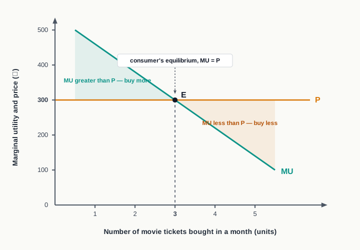
Fig. 3.3 – Consumer’s equilibrium in the one commodity case.
To the left of E the marginal utility curve lies above the price line. Every ticket in that stretch is worth more than it costs, so the consumer keeps buying and moves rightward. To the right of E the curve lies below the price line and each ticket costs more than it is worth, so the consumer draws back. Only at E, where the curve cuts the price line, is there no reason to move in either direction.
3.4 The Law of Equi-Marginal Utility
A consumer with an income of a few thousand rupees a month does not spend it on one commodity. The income has to be divided among many, and however large it is, it is never large enough for everything wanted. The constraint that matters here is therefore not the price of a single good but the budget as a whole.
This changes the question. In Section 3.3 the consumer had to decide how far to carry the purchase of one commodity. Now the decision is how to split a fixed sum between commodities, and a rupee given to one is a rupee denied to the other. The law of equi-marginal utility states the rule by which a rational consumer makes that split.
3.4.1 Statement of the Law
The law is also stated as a rule of proportions. The marginal utility of a rupee spent on a commodity is its marginal utility divided by its price, so saying that the last rupee spent on each good yields the same utility is the same as saying that the marginal utility of each good is proportional to its price. This second form is called the proportionality rule.
3.4.2 Consumer’s Equilibrium With Two Commodities
The magnitude the consumer works with is the utility obtained from the last rupee spent on a commodity. It is found by dividing the marginal utility of the commodity by its price, because the price is the number of rupees that last unit absorbed.
The consumer is in equilibrium when the last rupee spent on each commodity brings in the same marginal utility.
\[\dfrac{MU_X}{P_X} = \dfrac{MU_Y}{P_Y} = MU_m\]
Here \(MU_X\) and \(MU_Y\) are the marginal utilities of the last units of commodities X and Y in utils, \(P_X\) and \(P_Y\) are their prices in rupees, and \(MU_m\) is the marginal utility of a rupee of money income, measured in utils per rupee. The equality is read as follows: the final rupee spent on X and the final rupee spent on Y do equally well for the consumer, so nothing is to be gained by moving a rupee from one to the other.
Proportionality by itself is not enough. The rule can be satisfied at several different combinations of the two goods, and the combination actually reached must also be affordable and must use up the whole income.
\[P_X \times Q_X + P_Y \times Q_Y = M\]
Here \(Q_X\) and \(Q_Y\) are the quantities of X and Y purchased, \(P_X\) and \(P_Y\) their prices in rupees, and \(M\) the consumer’s money income in rupees. A combination costing less than \(M\) leaves income unspent and utility unclaimed; a combination costing more is out of reach.
Why The Equality Must Hold
Suppose the last rupee spent on X yields 8 utils while the last rupee spent on Y yields 5. The consumer has not yet arrived at the best arrangement, because a rupee taken away from Y loses 5 utils and the same rupee spent on X gains 8, a net addition of 3 utils.
The transfer does not continue indefinitely. As more of X is bought, the law of diminishing marginal utility pulls the marginal utility of X down, and as less of Y is bought, the marginal utility of Y rises. The gap narrows from both sides and closes when the two ratios are equal. At that point no further transfer can add anything, and the consumer is in equilibrium.
3.4.3 Equilibrium Explained by Schedule and Diagram
Table 3.5 sets out the marginal utility a student derives from pens priced at ₹4 each and chart papers priced at ₹8 each, together with the marginal utility per rupee spent on each. The student has ₹32 to divide between the two.
Both per-rupee columns fall as the quantity rises, which is diminishing marginal utility showing through after the division by price. The proportionality rule is met at more than one place: 3 pens with 1 chart paper give 8 utils per rupee on each, 4 pens with 2 chart papers give 7, and 5 pens with 3 chart papers give 6. Only one of these can be bought with ₹32, and SE 3.7 identifies it.
The working is shown graphically in Fig. 3.4, where the marginal utility per rupee of each commodity is measured on the vertical axis of its own panel, so that the level at which the two are equal can be read straight across.
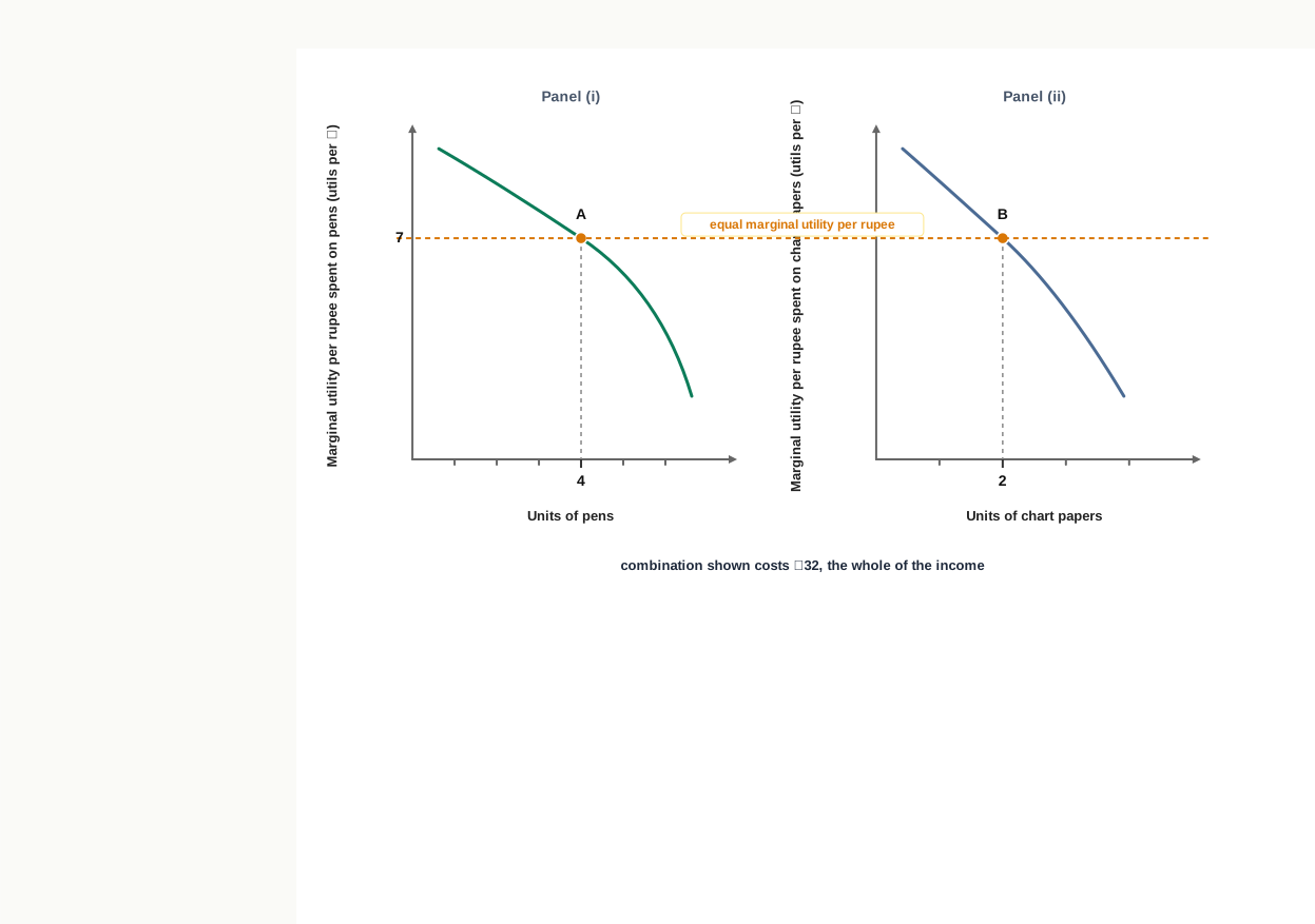
Fig. 3.4 – Operation of the law of equi-marginal utility.
3.4.4 Limitations of the Law
The law tells a consumer how a limited income ought to be divided, and as a rule of conduct it is sound. Applying it exactly is another matter, and five difficulties are usually pointed out.
- Utility cannot in fact be measured — the consumer cannot read off the marginal utility of a commodity in utils, so the ratios the law compares are never actually worked out.
- Purchases are governed by habit and custom — a great deal of household spending follows what has always been bought or what an occasion demands, rather than a fresh weighing of satisfaction against price.
- Consumers are often ignorant — a buyer who does not know the prices of substitutes, or the uses a commodity can be put to, cannot arrive at the position the law describes.
- Some goods are indivisible — a refrigerator or a car is bought whole or not at all, so it means little to speak of adjusting the last rupee spent on it. The law applies best to goods that can be bought in small quantities.
- The marginal utility of money is not constant — as a consumer spends, the money still in hand grows scarcer and each remaining rupee comes to matter more, which the law assumes away.
These difficulties do not rob the law of its value, since it still describes the direction in which a rational consumer moves. They do point to something else. An analysis that requires satisfaction to be counted in units is resting on a good deal that it cannot deliver, and that objection led economists to look for an approach asking the consumer only to rank alternatives. That approach is taken up next.
3.5 Ordinal Utility and the Indifference Curve
The whole of the cardinal analysis rests on one demanding assumption: that a consumer can say how much satisfaction a commodity gives, in numbers. The limitations set out in Section 3.4.4 show how heavy that assumption is. Satisfaction is a mental state, and no consumer leaves a shop able to report that the purchase yielded 34 utils.
Modern demand theory therefore asks for much less. It asks only that the consumer be able to compare bundles of goods and say which is preferred, or that the two are equally good. This is the ordinal approach, and the tool built on it is indifference curve analysis. The indifference curve was first drawn by the Italian economist Pareto, and the analysis was developed in its full form by the British economists J. R. Hicks and R. G. D. Allen.
3.5.1 From Cardinal Utility to Ordinal Utility
Cardinal utility means utility measured in absolute numbers, in the way height, weight or temperature is measured. A consumer working with cardinal utility must be able to say that one mango gives 20 utils and a second gives 15.
Ordinal utility means utility expressed as a rank order. The word ordinal refers to ordering — first, second, third. A consumer working with ordinal utility need only place bundles in order of preference, and need not say by how much one is better than another. Ranking is something every consumer does; measuring is not.
The list a consumer draws up in this way is called the scale of preference. It shows, for any two bundles of goods, either that one is preferred to the other or that the consumer is indifferent between them. This is a far less restrictive requirement, which is why the ordinal approach is regarded as the stronger of the two. The main points of difference between the two approaches are set out below.
3.5.2 Indifference Schedule and Indifference Curve
Take a household choosing between two goods, rice and pulses. Several combinations of the two can be put before it, each with more of one good and less of the other, arranged so that the household regards them all as equally good. Such a list is an indifference schedule.
Table 3.6 gives such a schedule. Each combination has one more kilogram of rice than the one before it, and enough pulses have been taken away to leave the household exactly as well off as before.
At combination A the household holds 1 kg of rice and 12 kg of pulses; at B it holds 2 kg of rice and 8 kg of pulses. Four kilograms of pulses have gone and one kilogram of rice has come in, and the household is no better and no worse off than before. The same is true of every step down the schedule. Nothing here is measured; the household has only been asked to say when two bundles are equally acceptable.
Plotting these combinations and joining them gives the curve shown in Fig. 3.5.
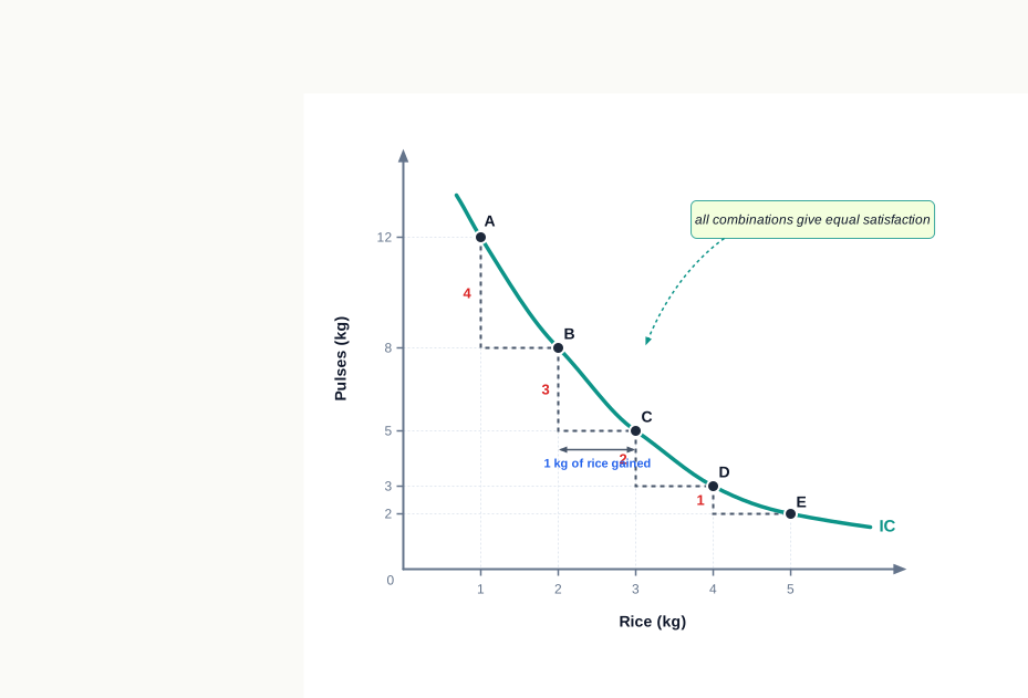
Fig. 3.5 – An indifference curve.
The curve slopes downward because more rice can be had only by giving up pulses if satisfaction is to stay the same. It is convex to the origin because the steps grow shorter as the household moves down it, a point taken up in Section 3.5.4 and again among the properties in Section 3.6.
3.5.3 Indifference Map
One indifference curve shows one level of satisfaction. A household is not confined to that level. Combinations with less of both goods can be listed, and they too will be equally good among themselves, giving a curve lying below the first. Combinations with more of both goods give a curve lying above it. Drawing a family of such curves in one diagram gives an indifference map.
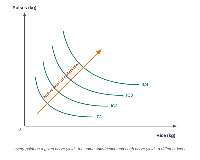
Fig. 3.6 – An indifference map.
Each curve on the map stands for one level of satisfaction, and the level rises as the curves move away from the origin. A point on IC3 has more of at least one good, and no less of the other, than a comparable point on IC2, so it must be preferred. The consumer would like to reach the highest curve possible; what prevents this is income, which the map does not show.
3.5.4 Marginal Rate of Substitution
The steps in Table 3.6 record something important. Each shows the quantity of pulses the household is willing to part with in exchange for one more kilogram of rice, with satisfaction unchanged. That rate of exchange is the marginal rate of substitution.
\[MRS_{XY} = \dfrac{\Delta Y}{\Delta X}\]
Here \(\Delta Y\) is the number of units of Y the consumer gives up and \(\Delta X\) the number of units of X gained, both measured in physical units of the goods. The result is read as so many units of Y per unit of X. Moving from A to B in Table 3.6, four kilograms of pulses are surrendered for one kilogram of rice, so the marginal rate of substitution is 4:1.
Read down the last column of Table 3.6 and the rate falls: 4, then 3, then 2, then 1. This tendency is called the diminishing marginal rate of substitution, and it has a straightforward reason behind it. As the household acquires more rice, each additional kilogram of rice meets a want that is already better met, so rice is valued less at the margin. At the same time its stock of pulses is shrinking, and the pulses that remain are put to more and more important uses, so each kilogram of pulses is valued more. A household that is short of pulses will not give them up as freely as one that has plenty.
The falling rate is what shapes the curve. A large sacrifice of pulses for the first extra kilogram of rice makes the curve steep at the top, and a small sacrifice for the last makes it flat at the bottom. A curve whose slope falls steadily as it is descended is convex to the origin.
3.5.5 Assumptions of Indifference Curve Analysis
The analysis rests on five assumptions, each doing a definite piece of work.
- Rationality — the consumer aims at the highest attainable indifference curve, given income and prices, and so acts to maximise satisfaction.
- Ordinal utility — satisfaction is taken to be capable of being ranked and not of being measured, which is what frees the analysis from the cardinal assumption.
- Non-satiety — the consumer is nowhere oversupplied and has not reached saturation in either good, so a larger quantity is always preferred to a smaller one. Without this, a bundle with more of both goods could not be said to be better.
- Transitivity of choice — if bundle A is preferred to B and B to C, then A must be preferred to C; and if the consumer is indifferent between A and B and between B and C, then A and C must be equally good. This keeps tastes consistent and the ranking free of contradiction.
- Diminishing marginal rate of substitution — the consumer gives up less and less of one good for each additional unit of the other. This is what makes the indifference curve convex to the origin.
With these assumptions the shape and position of the curves are settled, and four properties follow from them. Those properties are the subject of the next section.
3.6 Properties of Indifference Curves
An indifference curve is not drawn in any shape that happens to be convenient. Its slope, its curvature and its position relative to other curves all follow from the assumptions set out in Section 3.5.5, and each of them can be traced back to one of those assumptions.
Four properties are established here. They matter for the analysis that follows, because the equilibrium of Section 3.8 depends on the curve having exactly this shape and on the curves being arranged in exactly this way.
3.6.1 An Indifference Curve Slopes Downward From Left to Right
Every indifference curve has a negative slope. Satisfaction has to remain the same at every point on it, and the only way to hold satisfaction constant while taking more of one good is to give up some of the other.
The reason lies in the assumption of non-satiety. Suppose a household took one more kilogram of rice while keeping its pulses unchanged. It would then hold more of one good and no less of the other, and by non-satiety it must be better off. A better-off position cannot lie on the same indifference curve, since every point on that curve gives the same satisfaction. The combination must therefore lie on a higher curve, as Fig. 3.7 shows.
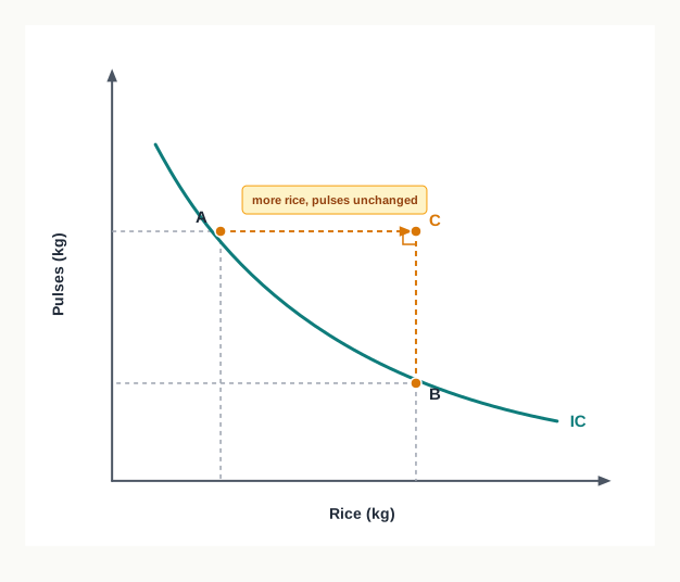
Fig. 3.7 – Why an indifference curve slopes downward.
A curve that sloped upward, or ran horizontally, would therefore contradict the assumption on which the analysis is built. Only a downward sloping curve can join combinations that are genuinely equal in the consumer’s eyes.
3.6.2 An Indifference Curve Is Convex to the Origin
Convexity means that the curve bows inward, towards the point of origin. The property follows directly from the diminishing marginal rate of substitution explained in Section 3.5.4.
The slope of an indifference curve at any point is the marginal rate of substitution at that point. If the rate at which the household is willing to give up pulses for rice falls as it acquires more rice, then the slope of the curve must be falling too. A curve that is steep at the top and grows flatter as it is descended is convex to the origin, and this is exactly what the steps in Fig. 3.5 show: four kilograms of pulses surrendered for the first extra kilogram of rice, then three, then two, then one.
The shapes that are ruled out make the point clearer. A straight line would mean a constant marginal rate of substitution, that is, a household willing to give up pulses at an unchanging rate however few it had left. A curve concave to the origin would mean an increasing rate, a household parting with pulses more and more freely as its stock of them ran down. Neither describes how consumers behave, which is why the normal indifference curve is drawn convex.
3.6.3 A Higher Indifference Curve Yields Higher Satisfaction
An indifference curve lying above and to the right of another represents a higher level of satisfaction. Every curve on the indifference map stands for one level, and the level rises as the curves move away from the origin.
Once again the reason is non-satiety. A combination on a higher curve contains more of one good and no less of the other, or more of both. Since a larger quantity is always preferred to a smaller one, that combination must be preferred. Fig. 3.8 sets two curves side by side to show this.
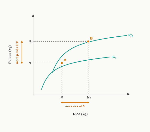
Fig. 3.8 – A higher indifference curve yields higher satisfaction.
At B the household has MM1 more rice and NN1 more pulses than at A. It is better supplied in both, so it must be better off, and IC2 must therefore represent a higher level of satisfaction than IC1. Every consumer would like to move to as high a curve as possible. What stops the movement is income, and that constraint enters the analysis in the next section.
3.6.4 Two Indifference Curves Never Intersect
Indifference curves may be drawn close to one another, but they can never cut or touch. Each curve represents a different level of satisfaction, and a single point cannot represent two different levels at once.
The property is best established by supposing the opposite. Let IC1 and IC2 cross at point P, as in Fig. 3.9, and take a point A on IC1 and a point B on IC2 standing above the same quantity of rice.
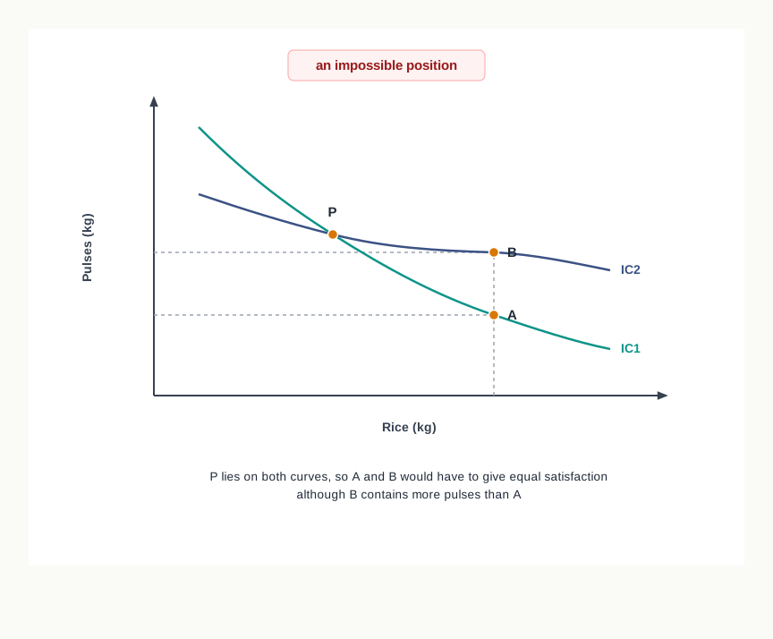
Fig. 3.9 – Two indifference curves cannot intersect.
The argument runs in three steps. P and A both lie on IC1, so they give equal satisfaction. P and B both lie on IC2, so they too give equal satisfaction. It follows, by transitivity, that A and B must give equal satisfaction. But B holds the same quantity of rice as A and more pulses than A, so by non-satiety B must be preferred to A. The two conclusions cannot both be true, and the contradiction arose from allowing the curves to cross. They cannot cross.
Two Further Points
Two smaller observations are worth adding to the four properties.
- Indifference curves do not touch either axis — the analysis assumes the consumer buys both goods, so every bundle contains some quantity of each. A curve touching an axis would mean a bundle made up of one good alone.
- Indifference curves need not be parallel — the slope of a curve at any point is the marginal rate of substitution there, and there is no reason for that rate to change at the same pace on every curve. The gap between two curves may widen or narrow.
3.7 The Budget Line
Indifference curves describe tastes. They say what a consumer would like, and they would say the same thing whether the consumer had ₹600 or ₹6,000 to spend. Left to itself, the indifference map offers no answer to the question this chapter set out to settle, because the consumer would simply climb to the highest curve on it.
What holds the consumer back is the constraint that opened the chapter: a fixed income and given prices. Two facts have therefore to be brought into the diagram — how much the household has to spend, and what the two goods cost. Together they define the set of combinations that can actually be bought, and the boundary of that set is the budget line.
3.7.1 Meaning and Construction of the Budget Line
Consider a household with ₹600 to spend in a week on rice priced at ₹30 a kilogram and pulses priced at ₹60 a kilogram. Spending the whole amount on pulses gives 10 kg of pulses and no rice. Spending it all on rice gives 20 kg of rice and no pulses. Between these two extremes lie several combinations, each using up the entire ₹600, and they are listed in Table 3.7.
Every combination in the table costs exactly ₹600, so each represents the largest quantity of the two goods the household can obtain at those prices. The relation the table expresses can be written as an equation.
\[P_X \times Q_X + P_Y \times Q_Y = M\]
Here \(Q_X\) and \(Q_Y\) are the quantities of the two goods purchased, \(P_X\) and \(P_Y\) their prices in rupees per unit, and \(M\) the consumer’s money income in rupees. Read as a statement about the household above, it says that ₹30 times the kilograms of rice plus ₹60 times the kilograms of pulses must come to ₹600.
Plotting these combinations and joining them gives Fig. 3.10.
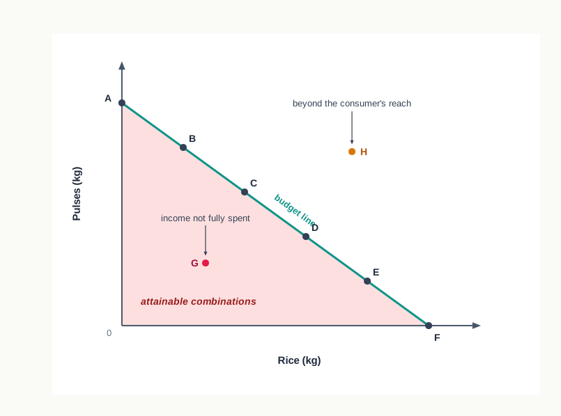
Fig. 3.10 – The budget line.
The line is drawn on two assumptions: that the consumer’s money income is fixed, and that the prices of the two goods are given. Everything on the line uses up the whole income. Everything inside the shaded area can be bought, but leaves part of the income unspent. Everything outside it, such as the point H, is beyond reach at the given income and prices.
3.7.2 Slope and Properties of the Budget Line
The budget line slopes downward for a plain reason. Income is fixed, so more of one good can be bought only by buying less of the other. How much less is decided by the two prices, and that is what the slope of the line records.
\[\text{Slope of the budget line} = -\dfrac{P_X}{P_Y}\]
Here \(P_X\) is the price of the good measured on the X-axis and \(P_Y\) the price of the good measured on the Y-axis, both in rupees per unit. For the household in Table 3.7 the slope is \(-30/60\), that is \(-0.5\). It is read as follows: one extra kilogram of rice costs the household half a kilogram of pulses, or, put the other way, giving up one kilogram of pulses releases enough money to buy two kilograms of rice. The minus sign records that one quantity rises only as the other falls.
The slope is thus the rate at which the market allows the two goods to be exchanged, in contrast with the marginal rate of substitution, which is the rate at which the consumer is willing to exchange them. Section 3.8 brings the two rates together.
The main properties of the budget line follow from its construction.
- It is negatively sloped — with income fixed, an increase in the quantity of one good must be matched by a decrease in the quantity of the other.
- Its slope equals the price ratio \(P_X / P_Y\) with a minus sign — the terms on which the market lets the consumer swap one good for the other are settled entirely by the two prices.
- It is a straight line — prices are assumed given and do not vary with the quantity purchased, so the rate of exchange is constant throughout its length.
- Points on the line exhaust the income, points inside it leave part of the income unspent, and points outside it are unattainable — the line is the boundary of what the consumer can afford.
When The Line Shifts Or Rotates
The budget line is fixed only so long as income and prices are fixed. If either changes, the line moves, and the way it moves depends on which of them changed.
- A change in income, prices unchanged — the line shifts to a new position parallel to the old one. A rise in income moves it outward and away from the origin, so more of both goods becomes affordable; a fall moves it inward. The slope is unaffected, since the price ratio has not changed.
- A change in the price of one good, income unchanged — the line rotates about the intercept on the other axis. A fall in the price of the good on the X-axis lets the consumer buy more of it while the maximum quantity of the other good stays as it was, so the line becomes flatter.
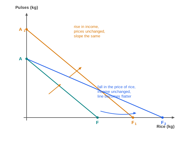
Fig. 3.11 – Shift and rotation of the budget line.
The distinction is worth holding on to. A change in income moves the whole line without altering its slope, because the market’s rate of exchange between the goods is untouched. A change in one price alters that rate of exchange, and so alters the slope itself.
With tastes represented by the indifference map and the constraint represented by the budget line, both halves of the consumer’s problem are now on the same diagram. The next section puts them together.
3.8 Consumer’s Equilibrium Under the Indifference Curve Approach
The two halves of the consumer’s problem are now in place. The indifference map shows what the household would like, ranking every combination of the two goods without measuring anything. The budget line shows what the household can do, given a fixed income and given prices.
Equilibrium is reached where these two meet. The consumer wants to climb to the highest indifference curve available, and the budget line marks how far the climb can go. The best position is therefore the highest indifference curve that the budget line can reach, and the consumer is in equilibrium there because no affordable rearrangement of purchases can do better.
3.8.1 Conditions of Equilibrium
Two conditions have to be satisfied at that position, and the second is as necessary as the first.
The First Condition
At the point of equilibrium the marginal rate of substitution between the two goods must equal the ratio of their prices.
\[MRS_{XY} = \dfrac{P_X}{P_Y}\]
Here \(MRS_{XY}\) is the number of units of Y the consumer is willing to give up for one more unit of X, while \(P_X\) and \(P_Y\) are the prices of the two goods in rupees per unit. The left-hand side is the rate at which the household is willing to exchange the goods; the right-hand side is the rate at which the market requires it to. Equilibrium is the quantity at which the two rates agree.
The reason is best seen by supposing they do not agree.
- When \(MRS_{XY}\) is greater than the price ratio — the household is willing to give up more of Y for a unit of X than the market actually demands. Buying more X and less Y therefore leaves it better off. As X is acquired, diminishing marginal rate of substitution pulls the MRS down towards the price ratio.
- When \(MRS_{XY}\) is less than the price ratio — the household values an extra unit of X at less than what the market charges for it in terms of Y. Buying less X and more Y leaves it better off, and the MRS rises towards the price ratio.
The adjustment stops only when the two are equal, which is what makes that quantity a position of rest. This condition is necessary, but it is not by itself sufficient.
The Second Condition
The indifference curve must also be convex to the origin at the point of equilibrium, that is, the marginal rate of substitution must be falling as the consumer moves down the curve.
The reason lies in what convexity guarantees. If the curve is convex, moving away from the tangency point in either direction along the budget line takes the household on to a lower curve, so it has every reason to come back. Equilibrium is then stable. If the curve were concave at that point, the tangency would be the worst position on the budget line rather than the best, and any movement away from it would take the household on to a higher curve. It would keep moving instead of settling, so there would be no equilibrium at all.
To these two conditions one requirement must be added, and it is the same one that appeared in the cardinal analysis: the consumer must be on the budget line and not inside it, since a combination inside leaves part of the income unspent and therefore leaves satisfaction unclaimed.
3.8.2 Equilibrium Explained by Diagram
Return to the household of Section 3.7, with ₹600 to spend on rice at ₹30 a kilogram and pulses at ₹60 a kilogram. Its budget line AF is drawn in Fig. 3.12 along with three curves from its indifference map.
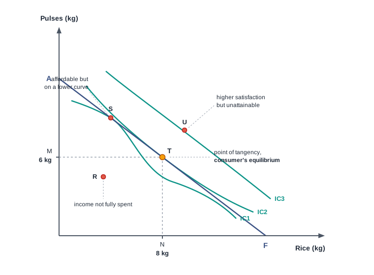
Fig. 3.12 – Consumer’s equilibrium under the indifference curve approach.
The household settles at T, buying 8 kg of rice and 6 kg of pulses, which costs exactly ₹600. Every other point on the diagram can be ruled out, and the reasons are worth taking one at a time.
- Point U lies on IC3 — it would give greater satisfaction than T, but it lies outside the budget line and cannot be bought at the given income and prices.
- Point R lies inside the budget line — it can be bought, but it leaves part of the ₹600 unspent and lies on IC1, a lower curve than IC2.
- Point S lies on the budget line — the whole income is spent there, but it lies on IC1. By moving along the line towards T the household reaches IC2, so S cannot be the best it can do.
At T the budget line is tangent to IC2, which means the slope of the curve equals the slope of the line at that point. The slope of the indifference curve is the marginal rate of substitution and the slope of the budget line is the price ratio, so at T the household is willing to give up half a kilogram of pulses for one more kilogram of rice, which is exactly what the market asks of it at prices of ₹30 and ₹60. There is nothing left to gain by any further exchange, and IC2 is the highest curve the household can reach.
Comparing The Two Approaches
The two routes taken in this chapter reach the same destination by different roads, and the differences between them were set out earlier in the chapter when cardinal and ordinal utility were distinguished.
The indifference curve approach is generally regarded as the stronger of the two. It makes fewer assumptions, and the assumptions it does make are less demanding: the consumer is asked only to rank combinations, not to measure satisfaction in utils, and the marginal utility of money is not required to stay constant. Its equilibrium condition is stated in terms of quantities the consumer actually compares, and it explains the effect of a price change on demand more generally. The point is often summed up by saying that indifference curve analysis assumes less and explains more, while marginal utility analysis assumes more and explains less.
That said, the cardinal approach is not discarded. It states the consumer’s problem in its simplest form, and the law of diminishing marginal utility on which it rests remains the reason a demand curve slopes downward. Both approaches, in the end, are answers to the question with which the chapter began: how does a consumer with limited means decide what to buy?
3.9 Summary
- Utility is the want-satisfying power of a commodity, that is, the satisfaction a consumer derives from consuming it. It is subjective, relative to the intensity of the want, not measurable in objective terms, different from usefulness and free of ethical connotations.
- Total utility is the satisfaction obtained from all the units of a commodity consumed, while marginal utility is the addition made to total utility by one more unit. Utility is measured in an imaginary unit called the util, or in money.
- Marginal utility is the difference between two successive figures of total utility: \(MU_n = TU_n - TU_{n-1}\), where \(MU_n\) is the marginal utility of the nth unit, \(TU_n\) the total utility from n units and \(TU_{n-1}\) the total utility from one unit less, all measured in utils.
- Total utility is the sum of the marginal utilities of every unit consumed: \(TU_n = MU_1 + MU_2 + \dots + MU_n = \Sigma MU\), where each term is the marginal utility of a successive unit in utils.
- The relationship between the two magnitudes runs in three stages.
- Total utility rises, though at a diminishing rate, so long as marginal utility is positive.
- Total utility is at its maximum when marginal utility is zero, and this is the point of satiety.
- Total utility falls when marginal utility becomes negative, and the commodity then yields disutility.
- The law of diminishing marginal utility states that as the amount of a commodity consumed increases, other things remaining equal, the utility derived from each additional unit goes on decreasing. It was given its systematic formulation by Alfred Marshall.
- The law holds only under its assumptions: identical units, a unit of standard size, unchanged tastes, continuity in consumption, unchanged prices of substitutes, measurable utility, a rational consumer and a constant marginal utility of money.
- Two explanations are given for the law: a particular want is satiable, and a commodity with several uses is applied first to the most urgent of them.
- In the one commodity case, a consumer is in equilibrium at the quantity where the marginal utility of the commodity, expressed in money, equals its price: \(MU_X = P_X\), both in rupees. Where \(MU_X > P_X\) the consumer buys more, and where \(MU_X < P_X\) the consumer buys less.
- The law of equi-marginal utility states that a consumer maximising total utility allocates income so that the last rupee spent on each commodity yields the same marginal utility: \(\dfrac{MU_X}{P_X} = \dfrac{MU_Y}{P_Y} = MU_m\), where \(MU_X\) and \(MU_Y\) are marginal utilities in utils, \(P_X\) and \(P_Y\) prices in rupees and \(MU_m\) the marginal utility of a rupee in utils per rupee.
- Proportionality by itself is not enough, since the whole income must also be spent: \(P_X \times Q_X + P_Y \times Q_Y = M\), where \(Q_X\) and \(Q_Y\) are the quantities bought, \(P_X\) and \(P_Y\) the prices in rupees and \(M\) the money income in rupees.
- The equi-marginal law is difficult to apply in practice because utility cannot be measured, purchases follow habit and custom, consumers are often ignorant, some goods are indivisible and the marginal utility of money does not stay constant.
- Ordinal utility requires the consumer only to rank combinations in order of preference rather than to measure satisfaction. An indifference schedule lists combinations of two goods that give equal satisfaction, and the indifference curve is its diagrammatic form.
- An indifference map is a set of indifference curves, each representing a different level of satisfaction, the level rising as the curves lie farther from the origin.
- The marginal rate of substitution is the rate at which a consumer will give up one good for one more unit of another with satisfaction unchanged: \(MRS_{XY} = \dfrac{\Delta Y}{\Delta X}\), where \(\Delta Y\) is the units of Y surrendered and \(\Delta X\) the units of X gained, both in physical units. It diminishes as more of X is acquired.
- Indifference curve analysis assumes rationality, ordinal utility, non-satiety, transitivity of choice and a diminishing marginal rate of substitution.
- Four properties follow from those assumptions.
- An indifference curve slopes downward from left to right, because more of one good must be matched by less of the other if satisfaction is to stay the same.
- It is convex to the origin, because the marginal rate of substitution diminishes.
- A higher curve yields higher satisfaction, because it offers more of at least one good and no less of the other.
- Two indifference curves never intersect, since a single point cannot represent two levels of satisfaction.
- The budget line shows the combinations of two goods a consumer can buy with a given income at given prices, and is the graph of \(P_X \times Q_X + P_Y \times Q_Y = M\). Its slope is \(-\dfrac{P_X}{P_Y}\), the negative of the price ratio, where \(P_X\) and \(P_Y\) are the prices in rupees per unit of the goods on the X-axis and Y-axis.
- A point on the budget line uses up the whole income, a point inside it leaves income unspent, and a point outside it is unattainable. A change in income shifts the line parallel to itself, while a change in one price rotates it and alters its slope.
- Under the indifference curve approach the consumer is in equilibrium where the budget line is tangent to the highest attainable indifference curve, and two conditions hold there.
- \(MRS_{XY} = \dfrac{P_X}{P_Y}\), so that the rate at which the consumer is willing to exchange the goods equals the rate at which the market allows it.
- The indifference curve is convex to the origin at that point, which makes the equilibrium stable.
- Both approaches answer the same question, but the indifference curve approach makes fewer and less restrictive assumptions and explains the effect of a price change more generally. It is often said to assume less and explain more, while marginal utility analysis assumes more and explains less.
3.10 Points to Ponder
- The law of diminishing marginal utility requires that the units be identical and that consumption be continuous. Think of the things a household actually buys in a month — a cake of soap, a bus pass, a cinema ticket — and ask how often those conditions really hold. If they seldom hold exactly, is the law still worth stating, and what does your answer suggest about the role of assumptions in economics?
- Marginal utility analysis assumes that the marginal utility of money stays constant. Does a hundred-rupee note mean the same to a household on the first of the month as it does on the twenty-eighth? If it does not, how much of the equi-marginal rule survives?
- The ordinal approach was preferred because it asks less of the consumer — ranking rather than measuring. Is a theory that assumes less always the better theory, or can a more demanding assumption earn its place by yielding sharper conclusions?
- Both approaches rest on a consumer who is rational and well informed. Advertising, festival discounts and buying because a neighbour has bought are ordinary facts of the market. Should the idea of rationality be widened to take them in, or should they be treated as departures from a rule that still describes the general case?
- A subsidy on one commodity lowers the price of that commodity alone and swings the household’s budget line, whereas a cash transfer of the same value shifts the line outward without altering its slope. Which of the two leaves the household on a higher indifference curve, and on what does the answer depend? Consider also why a government might still prefer the subsidy.
- Indifference curve analysis takes the consumer’s preferences as given and never asks where they came from. If tastes are themselves shaped by income, by advertising and by the society a person lives in, how much of the consumer’s choice has the theory genuinely explained?
3.11 Objective Questions
- When the total utility derived from a commodity is falling, the marginal utility of the last unit consumed is: [1]
- zero
- positive but diminishing
- negative
- at its maximum
- Read the assertion and the reason given below and choose the correct option. [1] Assertion (A): A consumer buying a single commodity stops at the quantity where its marginal utility equals its price. Reason (R): Beyond that quantity the marginal utility of an additional unit is less than the price paid for it.
- Both (A) and (R) are true, and (R) is the correct explanation of (A).
- Both (A) and (R) are true, but (R) is not the correct explanation of (A).
- is true but (R) is false.
- Both (A) and (R) are false.
- Fill in the blank: the slope of the budget line is equal to the negative of the ______ of the two commodities. [1]
- State whether the following statement is true or false: two indifference curves may touch each other at one point although they cannot cross. [1]
- Match each item in Column 1 with the item in Column 2 that describes it. [1]
| Column 1 | Column 2 |
|---|---|
| a. Indifference map | i. The slope of an indifference curve |
| b. Marginal rate of substitution | ii. A combination at which the whole income is not spent |
| c. A point lying inside the budget line | iii. A set of curves, each representing a different level of satisfaction |
3.12 Check Your Concepts
- Define the marginal rate of substitution and state why it diminishes as a consumer moves down an indifference curve. [2]
- The total utility a consumer obtains from one, two, three and four units of a commodity is 25, 45, 60 and 68 utils respectively. Calculate the marginal utility of each unit and state whether the schedule conforms to the law of diminishing marginal utility. [3]
- State the two conditions that must be satisfied for a consumer to be in equilibrium under the indifference curve approach, and explain why the first condition by itself is not sufficient. [4]
- State the law of equi-marginal utility. A consumer has ₹24 to spend on two goods X and Y, priced at ₹4 and ₹2 per unit respectively. The marginal utility obtained from successive units of X is 40, 32, 24, 16 and 8 utils, and from successive units of Y it is 20, 16, 12, 8 and 4 utils. Explain how the consumer reaches equilibrium and state the combination that will be bought. [6]
3.13 Case-Based Question
- Meera runs a small tailoring unit and sets aside ₹1,200 every month for two inputs, thread and lining cloth. Thread costs ₹40 a reel and lining cloth ₹120 a metre. This month the price of lining cloth falls to ₹80 a metre, while the amount she sets aside and the price of thread remain unchanged.
- Explain what happens to Meera’s budget line after the fall in the price of lining cloth, and why its slope changes. [2]
- Meera says that combinations of thread and cloth which were beyond her reach last month are now available to her. Using the idea of attainable combinations, state whether she is right and give the reason. [2]