Chapter 4: Elasticity of Demand
When petrol prices rise, most vehicle owners fill their tanks much as before. When an airline cuts fares on the same route in a lean month, seats fill quickly. The law of demand tells us the direction of that response: quantity demanded moves opposite to price. It does not tell us by how much. For a household spending a fixed income, for a firm deciding whether a price cut will pay for itself, and for a government choosing which goods to tax, the size of the response is the whole question. Elasticity of demand is the tool economics uses to answer it, and it turns the law of demand from a qualitative statement into a quantitative one. Because it compares proportionate changes, the measure does not depend on the units in which price and quantity are recorded. Fig. 4.0 sets the two cases side by side: one steep demand curve, one flat, and the same fall in price drawn against each. This chapter defines elasticity of demand, sets out its degrees, works through the three methods of measuring it, examines what makes one good’s demand more elastic than another’s, and takes up income and cross elasticity.
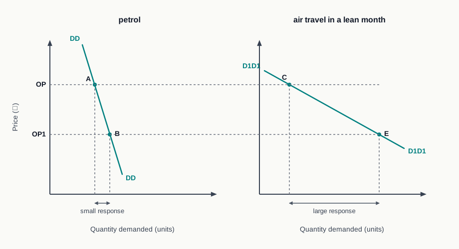
Fig. 4.0 – The same fall in price, two different responses.
4.1 Meaning and Types of Elasticity of Demand
The law of demand settles the direction in which a buyer moves: when the price of a commodity falls more of it is bought, and when the price rises less of it is bought. That is a qualitative statement. It does not say whether a ten per cent fall in price will bring one more unit into the market or a thousand. The gap matters because most decisions that rest on the law of demand turn on the magnitude rather than the direction. A firm cutting its price needs to know whether the extra units sold will more than make up for the lower price earned on every unit. A government taxing a commodity needs to know whether buyers will pay the higher price or leave the market. Both questions are about size, and the law of demand answers neither. Economics answers them with a ratio. Rather than set the change in quantity against the change in price in their own units — litres against rupees — it compares the proportionate change in the one with the proportionate change in the other. What comes out is a pure number, and pure numbers can be placed side by side across commodities that are counted in quite different ways.
4.1.1 Meaning of Elasticity of Demand
Demand for a commodity is governed by several determinants: its own price, the prices of related commodities, the income of the consumer, tastes, and the number of buyers in the market. A change in any one of them, the rest held constant, will move the quantity demanded. Elasticity of demand measures how far the quantity moves.
Three features of the measure should be fixed at the outset. 1. A ratio of proportionate changes — the change in quantity is expressed as a fraction of the original quantity, and the change in the determinant as a fraction of its original value, so that the two are compared on the same footing. 2. A pure number — because both terms of the ratio are proportions, the units in which price and quantity happen to be recorded cancel out. Elasticity for rice sold in kilograms can therefore be set beside elasticity for petrol sold in litres. 3. Measured ceteris paribus — only one determinant is allowed to change at a time. If income and price moved together, the change in quantity could not be traced to either of them.
4.1.2 Types of Elasticity of Demand
Since responsiveness can be measured against any determinant, there are in principle as many elasticities of demand as there are determinants of demand. Three of them are studied at this level. 1. Price elasticity of demand — the responsiveness of the quantity demanded of a commodity to a change in its own price. 2. Income elasticity of demand — the responsiveness of the quantity demanded of a commodity to a change in the income of the consumer. 3. Cross elasticity of demand — the responsiveness of the quantity demanded of one commodity to a change in the price of a related commodity.
The classification is set out in Fig. 4.1.
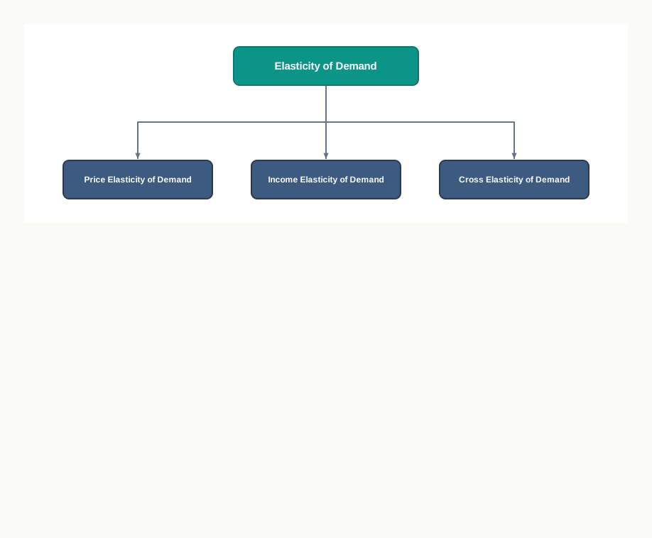
Fig. 4.1 – Types of elasticity of demand.
Of the three, price elasticity of demand is by far the most used, because price is the determinant that a seller can alter and a tax authority can influence. Sections 4.2 to 4.4 take it up in detail; income elasticity and cross elasticity follow in 4.5 and 4.6.
4.2 Price Elasticity of Demand
Of the determinants of demand, price is the one a seller can move at will and a government can influence through a tax. It is also the one whose effect on quantity is asked about most often. Price elasticity of demand is the measure built for that question.
4.2.1 Meaning of Price Elasticity of Demand
Two commodities may both obey the law of demand and still behave very differently when their prices fall by the same proportion. Buyers of one may take only a little more; buyers of the other may take a great deal more. Price elasticity of demand records the difference between them as a number.
Price elasticity of demand measures how sharply buyers respond to a change in price. It sets the proportionate change in quantity demanded against the proportionate change in price, so that the answer does not depend on the units in which either is recorded. \[e_p = \dfrac{\text{Percentage change in quantity demanded}}{\text{Percentage change in price}}\] Writing each percentage change out in full and cancelling the hundreds gives the form used in calculation. \[e_p = \dfrac{\Delta Q / Q}{\Delta P / P} = \dfrac{\Delta Q}{\Delta P} \times \dfrac{P}{Q}\] Here \(\Delta Q\) is the change in quantity demanded and \(Q\) the original quantity, both counted in units of the commodity; \(\Delta P\) is the change in price and \(P\) the original price, both in rupees. Because the units cancel, \(e_p\) is a pure number. The larger it is, the more sensitive buyers are to a change in price. One point of arithmetic should be settled before any calculation is attempted. Price and quantity move in opposite directions, so one of \(\Delta P\) and \(\Delta Q\) is always negative and \(e_p\) therefore works out to a negative value. Economists take the magnitude and drop the sign once the calculation is finished, and an elasticity written as \(1.5\) is understood to stand for \(-1.5\). The numerical value so obtained runs from zero at one extreme to infinity at the other.
4.2.2 Degrees of Price Elasticity of Demand
Between zero and infinity, the numerical value of \(e_p\) falls into five recognised degrees. Each is a statement about how the proportionate change in quantity compares with the proportionate change in price that produced it. 1. Perfectly inelastic demand (\(e_p = 0\)) — quantity demanded does not change at all when price changes. The same amount is bought whether the price rises or falls. Cases are rare even among necessities, since demand for food does alter somewhat with price; a life-saving medicine is the closest real instance. 2. Inelastic demand (\(e_p < 1\)) — quantity demanded changes by a smaller proportion than price. A fall in price of ten per cent that raises quantity by eight per cent gives \(e_p = 0.8\). Demand for necessities is generally inelastic. 3. Unitary elastic demand (\(e_p = 1\)) — quantity demanded changes by exactly the same proportion as price. A ten per cent fall in price raises quantity by ten per cent. This is the dividing line between the elastic and the inelastic cases. 4. Elastic demand (\(e_p > 1\)) — quantity demanded changes by a larger proportion than price. A fall in price of ten per cent that raises quantity by fifteen per cent gives \(e_p = 1.5\). Demand for luxuries is generally elastic. 5. Perfectly elastic demand (\(e_p = \infty\)) — buyers will take everything they can get at the ruling price and nothing at all at a price even slightly higher. A very small fall in price raises quantity demanded without limit. This is the upper extreme, and cases of it are extremely rare.
The Two Extreme Cases
The first and the last of these are limiting cases rather than descriptions of ordinary markets, and they are drawn as straight lines. Perfectly inelastic demand is a vertical line, because quantity stays at one figure whatever the price; perfectly elastic demand is a horizontal line, because the whole quantity is taken at one price and none at any other. Fig. 4.2 shows the two together.
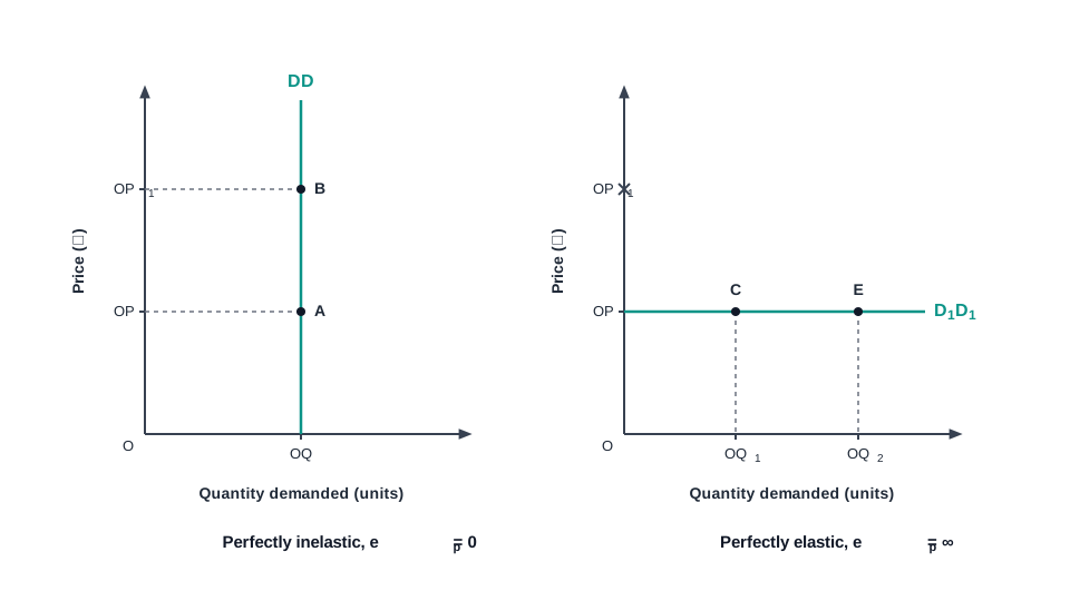
Fig. 4.2 – Perfectly inelastic and perfectly elastic demand.
The Unitary Elastic Case
Unitary elastic demand also has a shape of its own. If quantity always changes in the same proportion as price, the two changes cancel and the amount spent on the commodity stays where it was. A curve with that property is a rectangular hyperbola: it falls steeply near the price axis, flattens as it moves right, and approaches both axes without ever touching them. Fig. 4.3 draws it, with two rectangles marked off to show that spending is unchanged.
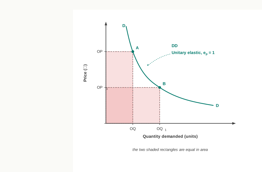
Fig. 4.3 – Unitary elastic demand.
Elastic And Inelastic Ranges
The three curves drawn so far are unusual in one further respect: each carries the same elasticity along its whole length. An ordinary demand curve does not. A downward sloping straight line has a constant slope, so equal falls in price bring equal rises in quantity all the way down it — yet its elasticity keeps changing. High on the curve the price is large and the quantity small, so a given change is a small proportion of the price and a large proportion of the quantity, and demand there is elastic. Low on the curve the position is reversed and demand is inelastic. Fig. 4.4 marks an elastic range and an inelastic range on one such curve.
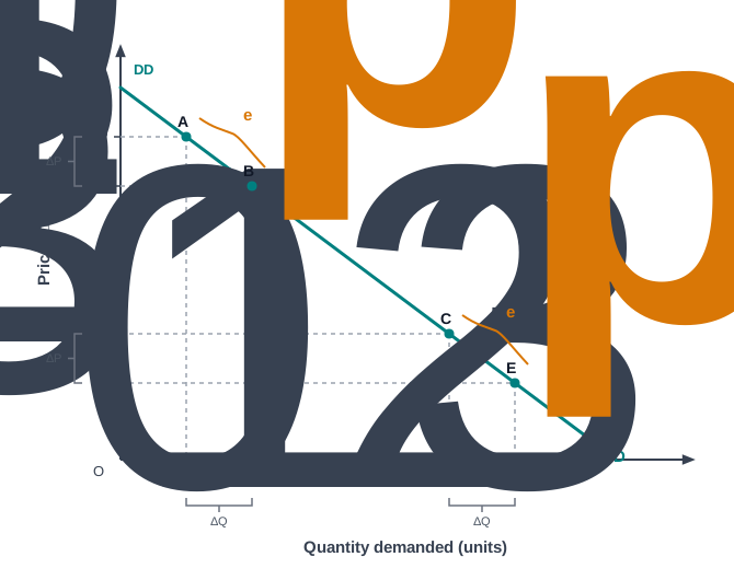
Fig. 4.4 – Elastic and inelastic ranges on a demand curve.
The five degrees are collected in Table 4.1.
It follows that a commodity cannot be labelled elastic or inelastic once and for all. The label belongs to a particular range of prices on a particular demand curve, and the same curve may earn both labels at different points along it.
4.3 Measurement of Price Elasticity of Demand
Knowing that demand for one good is elastic and for another inelastic is of little use until the two can be compared. A seller choosing between a price cut on soap and a price cut on cooking oil, or a finance minister choosing which of the two to tax, needs a figure for each. Measurement turns the five degrees of the previous section into numbers that can be set side by side. Before the measuring is done, one question has to be settled: is elasticity being measured at a single price, or over a stretch of the demand curve between two prices? The answer decides which method suits the case. Three methods are in use. 1. Percentage or proportionate method — the ratio of the percentage change in quantity demanded to the percentage change in price. 2. Total expenditure method — a comparison of the amount spent on the commodity before and after the price change. 3. Geometric or point method — the ratio of the two segments into which a chosen point divides a straight line demand curve.
4.3.1 Point Elasticity and Arc Elasticity
Elasticity can be looked at from two viewpoints. When the change in price is very small, so small that the movement along the curve is scarcely a movement at all, elasticity is being measured at a point. When the change is large enough to carry the buyer some distance down the curve, elasticity is being measured over an arc — the stretch of curve lying between the two positions.
Fig. 4.5 shows both on one curve: a point R, and the arc running from R to R1.
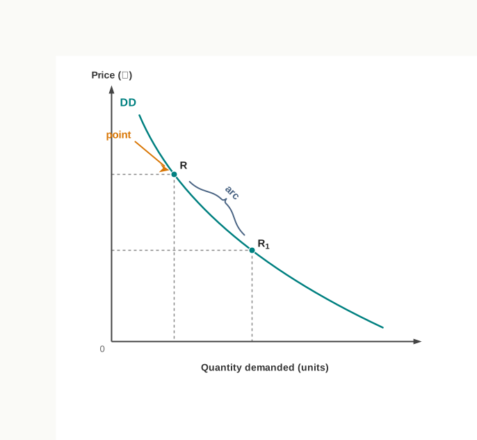
Fig. 4.5 – Point elasticity and arc elasticity.
The distinction matters in practice: the percentage and total expenditure methods both work from two positions and so yield arc elasticity, while the geometric method reads point elasticity off a single position on the curve.
4.3.2 Percentage or Proportionate Method
This is the method the definition itself suggests, and the only one on which numericals are set. Elasticity is measured by dividing the percentage change in quantity demanded by the percentage change in price. \[e_p = \dfrac{\Delta Q}{\Delta P} \times \dfrac{P}{Q}\] Here \(\Delta Q\) is the change in quantity demanded and \(Q\) the original quantity, both in units; \(\Delta P\) is the change in price and \(P\) the original price, both in rupees. The answer is a pure number, read against the five degrees of Table 4.1. Three steps make the working safe. Write down \(P\), \(Q\), \(\Delta P\) and \(\Delta Q\) before anything else; take the original values as the base for both proportions; and carry the negative sign through the arithmetic, removing it only when the answer is stated. SE 4.1 applies the formula to a rise in price.
The same formula answers the question the other way round. If elasticity is already known, the quantity that will be bought at a new price can be worked out from it, as in SE 4.2.
One limitation of the method should be noted. When the two prices are far apart, the answer depends on which pair of values is treated as the base, since the same absolute change is a different proportion of the old price and of the new. Statisticians meet this by averaging the two, but at this level the original values are always taken as the base.
4.3.3 Total Expenditure Method
Marshall’s own test does away with percentages. Total expenditure, or total outlay, is the amount households spend on a commodity, and it is simply price multiplied by quantity. \[TE = P \times Q\] Here \(TE\) is total expenditure in rupees, \(P\) the price per unit in rupees and \(Q\) the quantity bought in units. When price changes, the two terms of this product move in opposite directions, and which of them wins decides what happens to the total. 1. Elastic demand — a fall in price raises total expenditure and a rise in price lowers it, because the change in quantity more than offsets the change in price. Total expenditure moves against the price, so \(e_p > 1\). 2. Inelastic demand — a fall in price lowers total expenditure and a rise in price raises it, because the change in price more than offsets the change in quantity. Total expenditure moves with the price, so \(e_p < 1\). 3. Unitary elastic demand — total expenditure is unchanged whichever way price moves, because the two changes exactly offset each other, so \(e_p = 1\).
The three cases are set out in Table 4.2, where the price of each commodity falls from ₹60 to ₹50 and the quantity bought at each price is recorded.
Spending on X rises with the fall in price, so demand for X is elastic. Spending on Y falls, so demand for Y is inelastic. Spending on Z is the same at both prices, so demand for Z is unitary elastic. Table 4.3 states the rule for a rise in price as well.
The method has one clear weakness. It tells us whether elasticity is greater than one, equal to one or less than one, but it does not give the value itself. Demand that yields \(e_p\) of 1.2 and demand that yields 4 are treated alike, since expenditure rises in both. For an exact figure the percentage method is needed.
4.3.4 Geometric or Point Method
The third method reads elasticity off the geometry of the demand curve itself, without any arithmetic on prices and quantities. Any point chosen on a straight line demand curve divides it into two segments: the part lying below the point, towards the quantity axis, and the part lying above it, towards the price axis. The ratio of the two gives the elasticity at that point. \[e_p = \dfrac{\text{Length of the segment below the point}}{\text{Length of the segment above the point}}\] Both terms are lengths measured along the demand curve, so the units cancel and the answer is again a pure number. The rule is easy to read: where the lower segment is the longer of the two, demand at that point is elastic; where it is the shorter, demand is inelastic.
4.3.4.1 Elasticity at Different Points on a Straight Line Demand Curve
Let AB be a straight line demand curve drawn from the price axis at A to the quantity axis at B, with D as its mid-point, as in Fig. 4.6. Applying the ratio at five positions gives five results. 1. At A, where the curve meets the price axis — the segment below is the whole line AB and the segment above has no length, so \(e_p = \dfrac{AB}{0} = \infty\). 2. At E, any point above the mid-point — the lower segment BE is longer than the upper segment EA, so \(e_p = \dfrac{BE}{EA} > 1\) and demand is elastic. 3. At D, the mid-point — the two segments are equal, so \(e_p = \dfrac{BD}{DA} = 1\) and demand is unitary elastic. 4. At C, any point below the mid-point — the lower segment BC is shorter than the upper segment CA, so \(e_p = \dfrac{BC}{CA} < 1\) and demand is inelastic. 5. At B, where the curve meets the quantity axis — the segment below has no length, so \(e_p = \dfrac{0}{AB} = 0\).
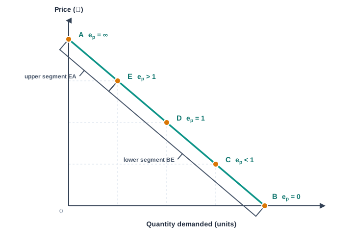
Fig. 4.6 – Price elasticity at different points on a straight line.
This is the geometric proof of a result stated earlier: as we travel down a straight line demand curve from left to right, elasticity falls steadily from infinity at the price axis to zero at the quantity axis, passing through unity at the mid-point. A straight line demand curve is therefore more elastic towards its upper end and less elastic towards its lower end.
4.3.4.2 Elasticity on a Non-Linear Demand Curve
Most demand curves are not straight lines, and a curved line has no segments to compare. The difficulty is got round by drawing a tangent. A tangent touches the curve at the chosen point and has the same slope there as the curve itself, so elasticity of the curve at that point equals elasticity of the tangent at that point — and the tangent, being a straight line, can be divided into segments in the usual way. Fig. 4.7 shows the construction at a point R.
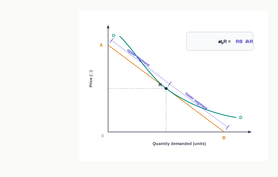
Fig. 4.7 – Price elasticity at a point on a non-linear demand curve.
The procedure is therefore the same in both cases: identify the point, obtain a straight line through it, and compare the segment below with the segment above.
4.4 Factors Affecting Price Elasticity of Demand
The coefficient of elasticity is not a number that has to be discovered afresh for every commodity. Much of it can be predicted from the character of the commodity itself and from the circumstances of the buyer, and that is why a firm can form a fair idea of the demand it faces before it ever changes a price. The question behind all of these determinants is the same. When the price of a commodity rises, what escape does the buyer have? Where an escape is easy — another commodity to turn to, another occasion to buy on, another use to give up — the quantity bought falls sharply and demand is elastic. Where there is no escape, the buyer pays and goes on buying, and demand is inelastic. The nine determinants below are so many descriptions of how much room the buyer has to move. 1. Availability of substitutes — this is the most important determinant of all. If a commodity has close substitutes, a rise in its price drives buyers to the substitute, quantity demanded falls steeply, and demand is elastic. If it has no good substitute, as with salt, buyers must go on buying it at whatever price rules, and demand is inelastic. The closer and the more numerous the substitutes, the more elastic the demand. 2. Nature of the commodity — a necessity is bought in more or less fixed quantities whether it is dear or cheap, because existence depends on it, so demand for foodgrains is inelastic. A comfort or a luxury is not essential, and its purchase can be dropped when it becomes dear, so demand for jewellery or an air conditioner is elastic. 3. Proportion of the income spent — the smaller the share of income a commodity takes, the smaller its elasticity. A household spends so little on a box of matches or a newspaper that a rise in price makes no perceptible difference to the budget, and the same quantity is bought. A scooter or a refrigerator absorbs a large part of income, so a change in its price is felt at once and demand for it is elastic. 4. Number of uses of the commodity — the greater the number of uses to which a commodity can be put, the greater its elasticity. Electricity can light a house, cook, heat water and run a pump. When it is dear it is kept for the most important of these uses only; as it grows cheaper it is extended to the less important ones as well, so the quantity taken changes a great deal with price. 5. Time factor — elasticity is generally low in a short period and higher in a long one. Tastes, habits and household routines take time to change, and new substitutes take time to appear. A rise in price therefore meets an inelastic demand at first, and a more elastic one as the months pass and buyers find their way to alternatives. 6. Possibility of postponement of consumption — where consumption can be put off, demand is elastic. A family can defer buying furniture or building a house until prices are easier, so a price rise produces a large fall in current purchases. Consumption of food cannot be postponed, and demand for it is inelastic for that reason alone. 7. Price range — demand tends to be inelastic at very high and at very low prices, and elastic in the moderate range between them. At a very high price only the rich buy, and a change leaves the commodity out of everyone else’s reach in any case. At a very low price everyone who wants the commodity already has it, so a further fall adds little. It is in the middle range, where a change in price brings fresh buyers into the market or drives them out, that elasticity is high. 8. Habits of the consumer — a commodity that has become habitual is bought almost without reference to its price. A regular user of tobacco does not greatly reduce his consumption when the price goes up, so demand for such commodities is inelastic. This is why an excise duty on them yields revenue rather than a fall in sales. 9. Income of the consumer — the same commodity may face different elasticities from different buyers. A rich household hardly notices a change in the price of an ordinary article and goes on buying the same quantity, so its demand is inelastic. For a middle-income or poor household the same change matters to the budget, and its demand is elastic.
The nine determinants are collected in Table 4.4, which states in each case the condition that makes demand elastic and the condition that makes it inelastic.
Two cautions follow from the list. First, the determinants work together and can pull against each other: a commodity may be a necessity, which makes for inelasticity, and yet have close substitutes, which makes for elasticity, and the net result depends on which pull is the stronger. Second, elasticity is not a permanent property of a commodity. It alters as incomes rise, as new substitutes are invented and as habits form, so a figure measured for one market in one period should not be carried over to another without thought.
4.5 Income Elasticity of Demand
Price is not the only thing that moves. Incomes rise as an economy grows, and households that could once afford only the necessities begin to buy other things as well. A firm planning a new factory, and a government forecasting the demand for foodgrains a decade ahead, both need to know which commodities that rising income will be spent on and which it will be taken away from. Income elasticity of demand is the measure that answers them.
The question is put exactly as it was for price. If the income of the consumer changes by a given percentage, by what percentage does the quantity demanded of the commodity change? The price of the commodity is held constant throughout, so that whatever change is observed can be credited to income alone.
Income elasticity of demand compares the proportionate change in quantity demanded with the proportionate change in income that brought it about.
\[e_y = \dfrac{\Delta Q}{\Delta Y} \times \dfrac{Y}{Q}\]
Here \(\Delta Q\) is the change in quantity demanded and \(Q\) the original quantity, both in units of the commodity; \(\Delta Y\) is the change in income and \(Y\) the original income, both in rupees. The result is a pure number, and it carries two pieces of information at once. Its sign says whether the commodity is one that buyers take more of or less of as they grow richer; its size says how strongly they respond. This is the point at which income elasticity parts company with price elasticity. There the negative sign was a nuisance to be dropped, since it merely repeated what the law of demand had already said. Here the sign is the finding itself, and it must be reported.
4.5.1 Types of Income Elasticity of Demand
Income elasticity of demand takes three forms, and the first of them divides further. 1. Positive income elasticity — quantity demanded rises as income rises and falls as income falls, so the two move together. Most commodities behave in this way, and goods that do are called normal goods. Within this class three degrees are distinguished. (a) Income elastic (\(e_y > 1\)) — quantity demanded rises by a larger proportion than income. Cars and meals taken in restaurants are of this kind, and so are luxuries generally. (b) Income inelastic (\(e_y\) positive but less than 1) — quantity demanded rises by a smaller proportion than income. Milk and other necessities are of this kind, since a household that grows richer does not drink proportionately more milk. (c) Unitary income elasticity (\(e_y = 1\)) — quantity demanded rises in exactly the same proportion as income. This is the dividing line between the two cases above rather than a class with many members in it. 2. Negative income elasticity (\(e_y\) less than zero) — quantity demanded falls as income rises, so the two move in opposite directions. Goods that behave in this way are called inferior goods. The buyer took them when he could afford nothing better and abandons them when he can, which is why less is bought at the higher income and more at the lower. 3. Zero income elasticity (\(e_y = 0\)) — a change in income leaves the quantity demanded exactly where it was. Toothpaste is an example: the amount a household uses is settled by habit and by the number of people in it, and a larger income beyond a certain point adds nothing to the quantity bought. Inexpensive essentials of this sort are the usual instances.
The five results are collected in Table 4.5.
Except for inferior goods and for inexpensive essentials, then, income elasticity of demand is positive for most commodities. The practical value of the measure lies in that qualification. A firm deciding whether to add to its capacity wants a product whose income elasticity is high, because rising national income will then carry its sales up with it; a firm whose product has a negative income elasticity must expect the opposite as the country grows richer.
4.6 Cross Elasticity of Demand
No commodity is bought in isolation. Some commodities compete with one another for the same place in the household’s basket, and others are of use only when they are bought together. Demand for a commodity therefore depends not only on its own price and on the buyer’s income, but on the prices of the commodities related to it. Cross elasticity of demand measures the strength of that connection. The question follows the pattern of the two before it. If the price of commodity Y changes by a given percentage, by what percentage does the quantity demanded of commodity X change? The price of X and the income of the consumer are held constant, so that the movement in X can be credited to the price of Y alone.
Cross elasticity of demand compares the proportionate change in the quantity demanded of X with the proportionate change in the price of Y that produced it.
\[e_{XY} = \dfrac{\Delta Q_X}{\Delta P_Y} \times \dfrac{P_Y}{Q_X}\]
Here \(\Delta Q_X\) is the change in the quantity demanded of commodity X and \(Q_X\) its original quantity, both in units of X; \(\Delta P_Y\) is the change in the price of commodity Y and \(P_Y\) its original price, both in rupees. The result is a pure number, and as with income elasticity the sign is the finding. A positive value says the two commodities are substitutes, a negative value that they are complements, and zero that they are not related at all. A single illustration fixes the reading. If the price of Y rises by ten per cent and the quantity of X demanded rises by four per cent as a result, then \(e_{XY} = 4 \div 10 = +0.4\): the two are substitutes, but weak ones, since buyers have shifted only a little. Had the same rise in the price of Y reduced the quantity of X demanded by four per cent, the answer would have been \(-0.4\) and the two would be complements.
4.6.1 Types of Cross Elasticity of Demand
Cross elasticity of demand takes three forms, and each of them identifies a different relation between the two commodities. 1. Positive cross elasticity — a rise in the price of Y raises the quantity demanded of X, and a fall in the price of Y lowers it. Quantity and price move in the same direction, so the sign is positive. Commodities that behave in this way are substitutes for one another, as two competing brands of soap are: when one brand is dearer, buyers simply take the other. The closer the substitutes, the larger the figure. 2. Negative cross elasticity — a rise in the price of Y lowers the quantity demanded of X, and a fall in the price of Y raises it. Quantity and price move in opposite directions, so the sign is negative. Commodities that behave in this way are complementary goods, which are used together: bread and butter are bought as a pair, so a fall in the price of butter raises the quantity of bread demanded as well. 3. Zero cross elasticity — a change in the price of Y leaves the quantity demanded of X exactly where it was. The two commodities are unrelated, neither standing in for the other nor being used alongside it. A wristwatch and a packet of biscuits are related in no way that a household’s budget records, and the cross elasticity between them is zero.
The three results are collected in Table 4.6.
The measure has a use beyond the classroom. A firm that finds a high positive cross elasticity between its product and a rival’s knows that the two are competing closely for the same buyers, and that it cannot raise its price without losing them; a firm whose product has a high negative cross elasticity with another knows that its own sales depend on what happens to the price of that other commodity, over which it has no control. The three elasticities studied in this chapter can now be set against one another. The main points of difference are given below.
4.7 Importance of Elasticity of Demand
A measure earns its place in economics by the decisions it improves. Elasticity of demand is used every time somebody has to guess what buyers will do next: a firm before it prints a new price list, a finance minister before he selects a commodity to tax, a trade union before it lodges a claim. In each case the same piece of information is wanted — will the quantity give way, and by how much? The uses set out below are the standard ones. They are worth reading as eight instances of a single idea rather than as eight separate facts.
Decisions Of The Firm
- Business decisions — a firm changing its price needs to know what will happen to its total revenue, and elasticity is what decides that. Raising the price adds to revenue only where demand is inelastic; where demand is elastic the sales lost outweigh the higher price, and revenue falls. Income elasticity serves the firm in a different way, by telling it whether demand for its product will grow as the country’s incomes grow, and so whether new capacity is worth building.
- Price discrimination by a monopolist — a seller who can keep his markets apart will not charge the same price in all of them. He charges the higher price where demand is inelastic, because little custom is lost by it, and the lower price where demand is elastic, because there the lower price brings in enough extra buyers to pay for itself. Without an estimate of elasticity in each market the policy cannot be framed.
Wages And Taxes
- Determination of factor prices — the strength of a trade union’s claim for higher wages rests on the elasticity of demand for the product its members make. If that demand is elastic, the higher wage raises the price of the product, sales fall away sharply, fewer workers are needed, and the claim is bought at the cost of jobs. If it is inelastic, the higher cost can be passed on to buyers without much loss of sales, and the union can bargain with effect.
- Formulation of government policy — a government that taxes a commodity in order to raise revenue chooses one whose demand is inelastic, since buyers will go on buying and the revenue will come in. A tax on a commodity with elastic demand drives the purchases away and the revenue with them. The same reasoning guides the granting of subsidies and the fixing of charges for public utilities such as electricity and transport.
- Incidence of taxation — the person on whom an indirect tax is levied is not always the person who ends by paying it. The more inelastic the demand, the larger the share of the tax the buyer bears, since he cannot easily do without the commodity; the more elastic the demand, the more of it the seller must absorb in order to keep his sales. This is why a government weighs elasticity before altering the rate on any commodity.
Trade, Currency And The Farm
- International trade — the terms of trade, which fix the rate at which a country’s exports exchange for its imports, depend on how elastic each country’s demand for the other’s goods is. A country whose exports meet an inelastic demand abroad is in the stronger position, since foreign buyers cannot easily turn elsewhere.
- Change in the rate of exchange — a devaluation makes a country’s exports cheaper to foreigners and its imports dearer at home. Whether that improves the balance of payments depends on elasticity: the quantities exported and imported must respond appreciably for the policy to work, and where demand on both sides is inelastic the change in price does little.
- Explanation of the paradox of plenty — a bumper crop, which ought to enrich the farmer, often leaves him worse off. Demand for agricultural produce is inelastic, so the extra output can be cleared only at a sharply lower price, and the fall in price more than cancels the rise in quantity. The paradox is entirely a consequence of inelastic demand.
Every one of these uses turns on the same question the chapter opened with. The law of demand tells the firm, the union and the government which way the quantity will move; only elasticity tells them whether the movement will be large enough to matter. That is why a concept introduced as a refinement of the law of demand has become one of the most heavily used tools in applied economics.
4.8 Summary
- The law of demand states only the direction in which quantity demanded moves when price changes. Elasticity of demand supplies the magnitude, and so turns a qualitative statement into a quantitative one.
- Elasticity of demand is the degree of responsiveness of the quantity demanded of a commodity to a change in any one of its determinants, other things remaining equal. Because it compares proportionate changes, it is a pure number that does not depend on the units in which price and quantity are recorded.
- Three elasticities are studied: price elasticity, measured against the commodity’s own price; income elasticity, measured against the income of the consumer; and cross elasticity, measured against the price of a related commodity.
- Price elasticity of demand is the ratio of the percentage change in quantity demanded to the percentage change in price: \(e_p = \dfrac{\Delta Q}{\Delta P} \times \dfrac{P}{Q}\), where \(\Delta Q\) is the change in quantity demanded, \(Q\) the original quantity in units, \(\Delta P\) the change in price and \(P\) the original price in rupees.
- Because price and quantity move in opposite directions, \(e_p\) works out negative. The convention is to complete the calculation and then report the magnitude alone.
- The numerical value of \(e_p\) runs from zero to infinity and is divided into five degrees.
- Perfectly inelastic, \(e_p = 0\) — quantity demanded does not change at all; the demand curve is a vertical line.
- Inelastic, \(e_p < 1\) — quantity changes by a smaller proportion than price; usual for necessities.
- Unitary elastic, \(e_p = 1\) — quantity changes in the same proportion as price; the demand curve is a rectangular hyperbola and total expenditure is unchanged.
- Elastic, \(e_p > 1\) — quantity changes by a larger proportion than price; usual for comforts and luxuries.
- Perfectly elastic, \(e_p = \infty\) — buyers take all they can get at the ruling price and nothing above it; the demand curve is a horizontal line.
- Point elasticity is measured at a single point on the demand curve; arc elasticity is measured over a finite stretch lying between two points. Throughout this chapter the original price and the original quantity are taken as the base.
- The percentage or proportionate method divides the percentage change in quantity demanded by the percentage change in price, using the formula of point 4. It is the method used in numericals, because it alone yields an exact coefficient from a pair of price and quantity figures.
- The total expenditure method compares the amount spent on the commodity before and after the price change, where total expenditure \(TE = P \times Q\), \(P\) being the price per unit in rupees and \(Q\) the quantity bought in units. It gives the category of elasticity but never its numerical value.
- Total expenditure moves in the direction opposite to price — demand is elastic, \(e_p > 1\).
- Total expenditure is unchanged — demand is unitary elastic, \(e_p = 1\).
- Total expenditure moves in the same direction as price — demand is inelastic, \(e_p < 1\).
- The geometric or point method reads elasticity off the demand curve as \(e_p = \dfrac{\text{Length of the segment below the point}}{\text{Length of the segment above the point}}\), both lengths being measured along the curve so that the scale cancels.
- On a straight line demand curve touching both axes, elasticity falls steadily as one moves down the curve: infinity where it meets the price axis, greater than one above the mid-point, unity at the mid-point, less than one below it, and zero where it meets the quantity axis. On a non-linear curve a tangent is drawn at the chosen point and the same ratio applied to the tangent.
- Nine determinants decide how elastic the demand for a commodity will be. Each of them is a statement about how much room the buyer has to escape a rise in price.
- Availability of substitutes — the closer and more numerous the substitutes, the more elastic the demand. This is the most important determinant.
- Nature of the commodity — necessities inelastic, comforts and luxuries elastic.
- Proportion of the income spent — the larger the share of income spent on the commodity, the more elastic the demand.
- Number of uses of the commodity — the more uses it has, the more elastic the demand.
- Time factor — demand is less elastic in a short period and more elastic in a long one.
- Possibility of postponement of consumption — demand is elastic where the purchase can be put off.
- Price range — demand is inelastic at very high and very low prices, elastic in the moderate range.
- Habits of the consumer — demand for a habitual commodity is inelastic.
- Income of the consumer — demand is inelastic for rich buyers and more elastic for middle-income and poor buyers.
- Income elasticity of demand is the ratio of the percentage change in quantity demanded to the percentage change in the income of the consumer: \(e_y = \dfrac{\Delta Q}{\Delta Y} \times \dfrac{Y}{Q}\), where \(\Delta Y\) is the change in income and \(Y\) the original income in rupees, the price of the commodity remaining unchanged. Here the sign is part of the answer and is never dropped.
- Positive — quantity rises with income; the commodity is a normal good. It is income elastic if \(e_y > 1\), as luxuries are; income inelastic if \(e_y\) is positive but less than one, as necessities are; and unitary if \(e_y = 1\).
- Negative — quantity falls as income rises; the commodity is an inferior good.
- Zero — quantity is unaffected by income, as with inexpensive essentials.
- Cross elasticity of demand is the ratio of the percentage change in the quantity demanded of one commodity to the percentage change in the price of a related commodity: \(e_{XY} = \dfrac{\Delta Q_X}{\Delta P_Y} \times \dfrac{P_Y}{Q_X}\), where \(\Delta Q_X\) and \(Q_X\) are the change in and the original quantity of X in units, and \(\Delta P_Y\) and \(P_Y\) the change in and the original price of Y in rupees. The sign again carries the finding.
- Positive — the two commodities are substitutes.
- Negative — the two commodities are complementary goods.
- Zero — the two commodities are unrelated.
- Elasticity of demand is used in taking business decisions and in fixing discriminatory prices, in judging the bargaining strength of a trade union, in framing tax and subsidy policy and deciding who bears an indirect tax, in the terms of international trade and the effect of a devaluation, and in explaining the paradox of plenty in agriculture.
The three methods of measuring price elasticity are set against one another below.
4.9 Points to Ponder
- A government seeking revenue is advised to tax commodities whose demand is inelastic, because buyers will go on buying them. But the commodities with the most inelastic demand are often the ones a poor household can least do without. Is a tax that is efficient at raising revenue necessarily a fair one, and how would you decide between the two claims?
- Every elasticity in this chapter was measured with income, tastes and the prices of related goods held constant. In an actual market all of them move at once, and the figures a firm works from are drawn from exactly such markets. How much confidence should a firm place in a coefficient estimated from data in which nothing was really held still?
- Because demand for farm produce is inelastic, a bumper harvest can leave farmers poorer, and a support price protects them from that outcome. It also keeps land and labour in a crop that buyers are not asking for in greater quantity. Which of the two losses should a government be more anxious to avoid?
- Elasticity on a straight line demand curve changes at every point, and yet firms and ministries speak of ‘the elasticity of demand’ for a product as though it were one number. What is that single number a statement about, and over what range of prices is it safe to rely on?
- Demand that is inelastic in a month may be elastic in a year, once buyers have found substitutes and altered their habits. Is elasticity then a property of the commodity at all, or only of the period we have chosen to look at — and what does that imply for a policy meant to last a decade?
4.10 Objective Questions
- A demand curve drawn parallel to the X-axis has a price elasticity of demand equal to: [1]
- zero
- one
- infinity
- less than one
- Read the Assertion (A) and the Reason (R) given below and choose the correct option. [1] Assertion (A): A commodity that can be put to a larger number of uses has a more elastic demand. Reason (R): As the price of such a commodity falls, it is put to its less important uses as well.
- Both Assertion (A) and Reason (R) are true, and Reason (R) is the correct explanation of Assertion (A).
- Both Assertion (A) and Reason (R) are true, but Reason (R) is not the correct explanation of Assertion (A).
- Assertion (A) is true, but Reason (R) is false.
- Assertion (A) is false, but Reason (R) is true.
- Fill in the blank: when a fall in the price of a commodity leaves the total expenditure on it unchanged, the price elasticity of demand for that commodity is equal to ________. [1]
- State whether the following statement is true or false: the income elasticity of demand for an inferior good is positive. [1]
- Match each item in Column 1 with the correct item in Column 2. [1]
| Column 1 | Column 2 |
|---|---|
| a. Perfectly inelastic demand | i. Positive cross elasticity of demand |
| b. Substitute goods | ii. \(e_p = 0\) |
| c. Mid-point of a straight line demand curve | iii. \(e_p = 1\) |
4.11 Check Your Concepts
- Define cross elasticity of demand and state the formula by which it is measured. [2]
- The price of a commodity falls from ₹25 to ₹20 per unit, and the quantity demanded rises from 80 units to 100 units. Calculate the price elasticity of demand by the percentage method and state its degree. [3]
- Explain any four factors that determine the price elasticity of demand for a commodity, giving one example of each. [4]
- Draw a downward sloping straight line demand curve touching both the axes. Mark on it the price elasticity of demand at the two ends, at the mid-point, and at one point above and one point below the mid-point, and explain why the value differs at each of them. [6]
4.12 Case-Based Question
- Meera Nathan runs Suraj Stationers, a small shop selling notebooks and printer cartridges. Last month she reduced the price of her notebooks from ₹50 to ₹40 each, and found that her takings from notebooks rose from ₹10,000 to ₹12,000 over the month. In the same month the company that makes the printers her customers own raised the price of those printers, and her sales of cartridges fell.
- Using the total expenditure method, state whether the demand for notebooks at her shop is elastic or inelastic, and give the reason for your answer. [2]
- What kind of cross elasticity of demand exists between the printers and the cartridges, and what does its sign tell Meera about the relation between the two? [2]