Chapter 6: Market Mechanism: Equilibrium Price And Quantity In A Competitive Market
Before most of the city is awake, trucks are unloading at the Azadpur mandi in Delhi, one of Asia’s largest wholesale markets for fruit and vegetables. Nobody announces the day’s rate for a crate of cauliflower. Buyers call out what they will pay, sellers hold out for more, and within a few hours trading settles at one rate that clears the morning’s arrivals. Earlier chapters studied the two sides of such a market separately. The demand curve showed how much buyers would take at each price; the supply curve showed how much sellers would offer. Neither curve on its own answers the question that matters most: what price will actually rule in the market, and how much will actually be bought and sold? Price is how a market economy solves a problem of coordination. Millions of buyers and sellers who never meet must somehow settle how much of a good is produced and who gets it, and the price that emerges does that work. This chapter explains how the market settles on a single price and quantity, how that outcome changes when demand or supply shifts, and what follows when a price is fixed by law.
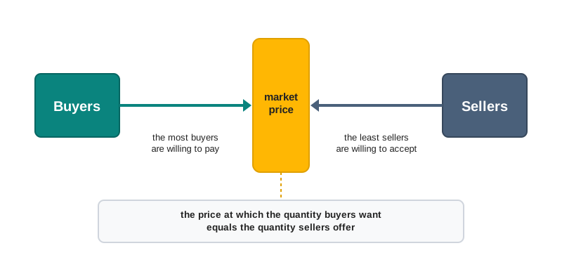
Fig. 6.0 – How a market price comes to be settled.
6.1 Equilibrium And Equilibrium Price
A demand curve and a supply curve each answer a conditional question. The demand curve states how much buyers would take at any given price; the supply curve states how much sellers would offer at that same price. Neither of them states what the price will actually be.
Scarcity is the reason a price is needed at all. There is not enough of the good to satisfy every buyer at a low price, and no seller will part with it at a price that fails to cover what it cost to make. The market settles the conflict by moving the price until the amount buyers want and the amount sellers offer are one and the same. This section builds the idea of that resting point and the vocabulary that goes with it; Section 6.2 then shows how a market arrives there.
6.1.1 The Meaning Of Equilibrium
Equilibrium is a general idea, borrowed by economics from the physical sciences. It means a state of balance: two forces working in opposite directions pull against each other until neither can move the other any further. A beam balance carrying equal weights in both pans is in equilibrium.
Two features of that state matter for economics. First, equilibrium is a position of rest, so once it is reached there is no tendency to move away from it. Second, the rest is not permanent. It lasts only as long as the forces producing it are unchanged; alter one of those forces and the balance is disturbed until a new position of rest is found.
Because equilibrium describes rest and nothing beyond it, the word carries no judgement about whether the outcome is a desirable one.
6.1.2 Equilibrium And Disequilibrium In A Market
In a market the two opposing forces are demand and supply. Buyers press the price down and sellers press it up, and balance is reached when the quantity demanded of the commodity equals the quantity supplied of it. That is what equilibrium means in the context of price determination.
When the two quantities are not equal, the market is in disequilibrium. One side of the market is then frustrated: either buyers cannot get all they want at the ruling price, or sellers cannot sell all they have offered. The frustrated side acts, by bidding more or by accepting less, and the price moves. Disequilibrium is therefore a state of motion, and it lasts only until the price has moved far enough to make the two quantities equal.
6.1.3 The Two Limits Within Which Price Settles
Before asking where the price settles, it is worth asking how far it can move at all. Each side of the market sets a limit beyond which it will not go, and any price actually agreed must lie between the two.
The Buyer’s Upper Limit
A buyer demands a commodity because it possesses utility, the power to satisfy a want. What he is prepared to pay for one more unit cannot exceed what that unit is worth to him, which is its marginal utility measured in money. He would like to pay as little as he can, but marginal utility fixes the highest price he can be induced to pay. Marginal utility therefore sets the upper limit of price.
The Seller’s Lower Limit
A seller supplies in order to earn a profit, and must recover what the unit cost him to produce. The least he can accept for one more unit is its marginal cost, since a price below that leaves him worse off for having produced the unit at all. He would like to charge as much as he can, but marginal cost fixes the lowest price he can be induced to accept. Marginal cost therefore sets the lower limit of price.
The two sides want opposite things, and each is checked by the other. The market reconciles them, and the price finally agreed is a price acceptable to both. It must lie in the band between the seller’s lowest limit and the buyer’s highest limit, as shown in Fig. 6.1.
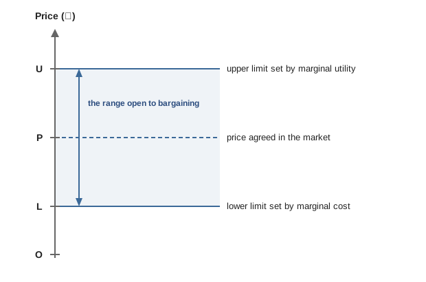
Fig. 6.1 – Range within which market price must lie.
6.1.4 Equilibrium Price And Equilibrium Quantity
Within that band there is one price at which the quantity buyers wish to buy is exactly the quantity sellers wish to sell. This is the equilibrium price, and it is the price the market is working towards whenever it is out of balance.
The equilibrium price is said to clear the market. At that price no seller is left with unsold stock, and no buyer who is willing and able to pay the price goes away without the good. Since neither side is frustrated, neither side has any reason to bid the price up or shade it down.
At every other price one side is frustrated, and the frustrated side sets the price moving again. That is why a price other than the equilibrium price cannot last, however long it may happen to rule for a while.
The amount that changes hands at the equilibrium price is the equilibrium quantity. Because the quantity demanded and the quantity supplied are equal at that price, a single figure measures both.
When the ruling price is the equilibrium price and the amount traded is the equilibrium quantity, price, demand and supply are all at rest together. The market is then said to be in market equilibrium.
6.2 Determination Of Equilibrium Price In A Competitive Market
In a competitive market there are many buyers and many sellers, and no one of them is large enough to move the price by his own decision. A single buyer who refuses to buy is replaced by another; a single seller who withholds his stock is replaced by another. Price is therefore not set by anybody. It is determined by the interaction of market demand and market supply, and every individual in the market takes it as given.
Two things are assumed throughout, both established in the earlier chapters. Market demand is inversely related to price, so a fall in price raises the quantity demanded. Market supply is directly related to price, so a rise in price raises the quantity offered. Putting the two together in one place shows the law of demand and the law of supply working against each other, and it is that opposition which fixes the price.
The determination can be shown in two ways: through the demand and supply schedules, which set out the quantities against each price, and through the demand and supply curves, which draw the same information. Both lead to the same answer.
6.2.1 Price Determination Through Demand And Supply Schedules
A market schedule places the two sides of the market side by side against the same list of prices. Consider the market for a standard school notebook in a town, where a large number of small firms print notebooks and a large number of households buy them. Table 6.1 shows how many thousand notebooks buyers would take each month at each price, and how many thousand sellers would offer.
Reading down the table, the two quantities are equal at one price only. At ₹40 buyers wish to take 30 thousand notebooks a month and sellers wish to offer exactly 30 thousand. The equilibrium price is therefore ₹40 and the equilibrium quantity is 30 thousand notebooks a month.
Every other price in the table is a disequilibrium price, because at each of them the quantity demanded and the quantity supplied are different numbers. The fourth column measures how different, and the last column states which way the price will be pushed as a result. The rest of the argument is simply an account of how that push works.
6.2.2 Excess Demand And Excess Supply
Consider first the prices below ₹40. At these prices buyers wish to buy more than sellers are willing to sell. At ₹30 buyers would take 40 thousand notebooks while sellers would offer only 20 thousand, leaving a gap of 20 thousand. The gap is called excess demand, and in the market it appears as a shortage of the commodity.
A shortage sets buyers against one another. There are not enough notebooks to go round at ₹30, so a buyer who is anxious to get them offers a little more rather than go without. Sellers, seeing that their stock is exhausted well before the queue is, begin to ask for more. For either reason, or both together, the price is bid up. As it rises the quantity demanded contracts and the quantity supplied expands, so the gap narrows. The rise continues until the gap has closed altogether, which happens at ₹40.
Now consider the prices above ₹40. At these prices sellers wish to sell more than buyers are willing to take. At ₹50 sellers would offer 40 thousand notebooks while buyers would take only 20 thousand, leaving 20 thousand unsold. This gap is called excess supply, and in the market it appears as a surplus lying with the sellers.
A surplus sets sellers against one another. A seller left with unsold notebooks would rather cut his price than carry the stock, and once one seller cuts, his rivals must follow or lose their customers altogether. Buyers, seeing stock lying unsold, hold back and offer less. The price is therefore pushed down. As it falls the quantity supplied contracts and the quantity demanded expands, and the surplus disappears at ₹40.
Notice that the two forces work in opposite directions and that both end at the same place. Whether the market starts too high or too low, it is driven towards ₹40, and once there it stops. The two states of disequilibrium are set out side by side below.
6.2.3 Diagrammatic Determination Of Equilibrium
The same determination can be shown with the market demand curve and the market supply curve drawn in one diagram. Quantity is measured along the X-axis and price along the Y-axis. The demand curve DD slopes downward from left to right, the supply curve SS slopes upward, and two curves sloping in opposite directions can cross at one point only. That single point of intersection is the equilibrium, as Fig. 6.2 shows. Both curves are drawn as straight lines here, which simplifies the drawing without changing the argument.
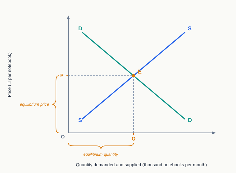
Fig. 6.2 – Equilibrium price and quantity.
At E the quantity demanded and the quantity supplied are both equal to OQ, and the price at which this happens is OP. Since the point lies on the demand curve, buyers are content to take OQ at that price; since it lies on the supply curve, sellers are content to offer OQ at that price. Neither side is asked to do anything it did not plan to do, which is why the position is one of rest.
Any other price can now be tested on the same diagram. Fig. 6.3 marks a price OP1 above OP and a price OP2 below it.
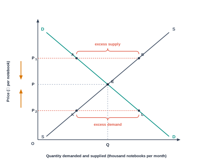
Fig. 6.3 – Excess supply and excess demand.
At the higher price OP1 the quantity demanded falls to P1A while the quantity supplied rises to P1B, so AB measures the surplus. Sellers competing to clear it force the price down towards OP. At the lower price OP2 the quantity supplied falls to P2K while the quantity demanded rises to P2L, so KL measures the shortage. Buyers competing to get the good force the price up towards OP. From either side the market moves to E, and only at E does it stay.
6.2.4 Stable Equilibrium
The equilibrium reached at E has a further property worth naming. If some small disturbance pushes the price away from OP, the market does not drift further away; the excess demand or excess supply created by the disturbance drives the price back. An equilibrium that repairs itself in this way is called a stable equilibrium.
It follows that neither force determines the price by itself. Demand alone cannot fix a price, because what buyers are willing to pay settles nothing unless sellers are willing to supply at it; supply alone cannot fix a price either, for the same reason in reverse. Both are necessary, and the price is the outcome of the two acting together.
One caution completes the account. The demand and supply model does not claim that the price ruling at every moment is the equilibrium price. Markets are frequently out of balance, and a price may stay away from equilibrium for some time. What the model claims is that whenever a market is out of balance, forces are set in motion that carry it towards equilibrium, through the ordinary process of haggling and bargaining between buyers and sellers.
6.3 Effect Of A Change In Demand On Equilibrium
The equilibrium reached in Section 6.2 was worked out for one given demand curve and one given supply curve. In practice the conditions lying behind those curves do not stay still. Incomes change, tastes change, the prices of related commodities change, the size of the population changes, and any of these will move the whole demand curve to a new position.
When the demand curve moves, the old equilibrium is no longer an equilibrium. At the price that used to clear the market, the quantity buyers now wish to take is no longer the quantity sellers wish to offer, so the market is thrown into disequilibrium and the price begins to move again. The question this section answers is where it comes to rest.
Throughout the section supply is taken to be unchanged, so that the effect of the demand side can be seen by itself. The supply curve SS therefore stays exactly where it is in both diagrams.
6.3.1 An Increase In Demand
An increase in demand means that buyers are willing to take a larger quantity at every price than before. It may follow from a rise in the income of consumers in the case of a normal good, a change in taste in favour of the commodity, a rise in the price of a substitute, a fall in the price of a complement, or a growth in the number of buyers. Whatever the cause, the whole demand curve shifts to the right, from D0D0 to D1D1 in Fig. 6.4.
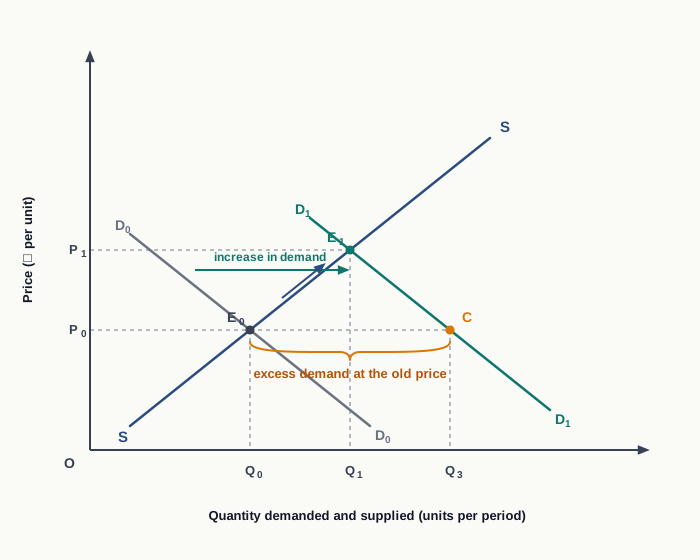
Fig. 6.4 – Effect of an increase in demand.
Take the market at its old equilibrium E0, with price OP0 and quantity OQ0. The shift does not change the price at once. At the price OP0 buyers now wish to take OQ3, while sellers, whose plans have not changed, still offer only OQ0. The distance E0C therefore measures the excess demand created by the shift.
That shortage sets the familiar adjustment going. Buyers compete for a quantity that is not enough to go round and bid the price up. As the price rises, the quantity demanded contracts along the new curve D1D1 and the quantity supplied expands along SS, so the gap narrows from both ends. The price stops rising only when the gap has closed, which happens at E1, where D1D1 cuts SS. The new equilibrium price is OP1 and the new equilibrium quantity is OQ1.
Both are higher than before. An increase in demand for a commodity, that is a rightward shift of the demand curve, causes an increase in both the equilibrium price and the equilibrium quantity bought and sold.
6.3.2 A Decrease In Demand
A decrease in demand means that buyers are willing to take a smaller quantity at every price than before. The causes are the reverse of those listed above: a fall in income in the case of a normal good, a change in taste against the commodity, a fall in the price of a substitute, a rise in the price of a complement, or a fall in the number of buyers. The demand curve shifts to the left, from D0D0 to D2D2 in Fig. 6.5.
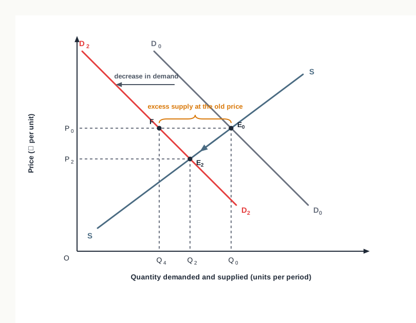
Fig. 6.5 – Effect of a decrease in demand.
At the old price OP0 sellers still offer OQ0, but buyers now wish to take only OQ4. The distance FE0 measures the excess supply created by the shift. Sellers left with unsold stock cut their prices against one another, and the price falls. As it falls the quantity supplied contracts along SS and the quantity demanded expands along D2D2, until the surplus disappears at E2.
The new equilibrium price is OP2 and the new equilibrium quantity is OQ2, both lower than before. A decrease in demand, that is a leftward shift of the demand curve, causes a decrease in both the equilibrium price and the equilibrium quantity bought and sold.
6.3.3 The Adjustment Process Step By Step
The move from one equilibrium to another is not instantaneous, and it is useful to set out the sequence in which it happens.
When Demand Increases
- The demand curve shifts to the right, supply remaining unchanged.
- Excess demand, that is a shortage, appears at the old price.
- Competition among buyers, and the willingness of sellers to ask for more, causes the price to rise.
- As the price rises the quantity supplied expands and the quantity demanded contracts, until the two are equal again at a higher price and a larger quantity.
When Demand Decreases
- The demand curve shifts to the left, supply remaining unchanged.
- Excess supply, that is a surplus, appears at the old price.
- Competition among sellers, and the unwillingness of buyers to pay the old price, causes the price to fall.
- As the price falls the quantity supplied contracts and the quantity demanded expands, until the two are equal again at a lower price and a smaller quantity.
Two points are worth holding on to. First, in both cases the equilibrium price and the equilibrium quantity move in the same direction, which is the direction in which demand itself has moved. Second, the whole adjustment takes place along the unchanged supply curve, so the size of the price change depends on how readily sellers can expand or contract output. The more responsive supply is, the smaller the change in price and the larger the change in quantity.
6.4 Effect Of A Change In Supply On Equilibrium
The demand side is now held still and the supply side allowed to move. A supply curve is drawn for given conditions of production, and those conditions change as often as the conditions behind demand do. A better technique, a change in the price of raw materials or fuel, a tax or a subsidy, the entry or exit of firms, and in the case of farm produce the weather, will each move the whole supply curve to a new position.
The reasoning runs exactly as before. At the price that used to clear the market, the quantity sellers now wish to offer is no longer the quantity buyers wish to take, so a shortage or a surplus appears and the price is set moving. Throughout this section the demand curve DD stays where it is.
6.4.1 An Increase In Supply
An increase in supply means that sellers are willing to offer a larger quantity at every price than before. It may follow from an improvement in the technique of production, a fall in the price of inputs, a reduction in tax or the grant of a subsidy, the entry of new firms into the industry, or a good harvest in the case of an agricultural commodity. The whole supply curve shifts to the right, from S0S0 to S1S1 in Fig. 6.6.
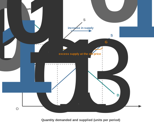
Fig. 6.6 – Effect of an increase in supply.
Begin at the old equilibrium E0, with price OP0 and quantity OQ0. At that price sellers are now prepared to offer OQ3, while buyers, whose plans are unchanged, still take only OQ0. The distance E0G measures the excess supply created by the shift.
The surplus sets sellers competing against one another. Each would rather cut his price than carry unsold stock, and the price falls. As it falls the quantity supplied contracts along the new curve S1S1 and the quantity demanded expands along DD, so the surplus shrinks from both ends. It disappears at E1, where DD cuts S1S1, giving a new equilibrium price OP1 and a new equilibrium quantity OQ1.
The two move in opposite directions. An increase in the supply of a commodity, that is a rightward shift of the supply curve, causes a decrease in the equilibrium price and an increase in the equilibrium quantity bought and sold.
6.4.2 A Decrease In Supply
A decrease in supply means that sellers are willing to offer a smaller quantity at every price than before. The causes are the reverse of those above: a rise in the price of inputs, an outdated or disrupted technique, a heavier tax or the withdrawal of a subsidy, the exit of firms from the industry, or a crop failure. The supply curve shifts to the left, from S0S0 to S2S2 in Fig. 6.7.
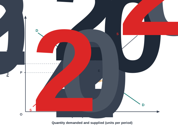
Fig. 6.7 – Effect of a decrease in supply.
At the old price OP0 buyers still wish to take OQ0, but sellers now offer only OQ4. The distance HE0 measures the excess demand created by the shift. Buyers compete for a quantity that no longer goes round and bid the price up. As the price rises the quantity demanded contracts along DD and the quantity supplied expands along S2S2, until the shortage disappears at E2.
The new equilibrium price OP2 is higher than OP0 and the new equilibrium quantity OQ2 is smaller than OQ0. A decrease in supply, that is a leftward shift of the supply curve, causes an increase in the equilibrium price and a decrease in the equilibrium quantity bought and sold.
6.4.3 Movement Along The Demand Curve
When the supply curve shifts, the whole adjustment takes place along the demand curve, which has not moved. A rightward shift of supply produces a downward movement along DD from E0 to E1; a leftward shift produces an upward movement along DD from E0 to E2. In each case buyers are not doing anything new. They are simply reading off the same demand curve at a different price.
This has a practical consequence worth noticing. How much of the adjustment shows up as a change in price, and how much as a change in quantity, depends on how responsive buyers are, that is on the elasticity of demand for the commodity.
- Where demand is inelastic — as it is for a necessity with few substitutes, a fall in supply is absorbed mainly by a sharp rise in price, because buyers reduce their purchases very little. This is why the failure of a single crop can send its price up steeply.
- Where demand is elastic — buyers switch readily to substitutes, so the same fall in supply is absorbed mainly by a fall in the quantity sold, and the price rises only a little.
The contrast with Section 6.3 should also be noted. When demand shifts, equilibrium price and equilibrium quantity move in the same direction. When supply shifts, they move in opposite directions. That difference is often the quickest way to work out which curve has moved when a question describes only the outcome: a rise in price together with a larger quantity sold points to demand, while a rise in price together with a smaller quantity sold points to supply.
6.5 Effect Of Simultaneous Changes In Demand And Supply
Sections 6.3 and 6.4 moved one curve at a time, holding the other still. That is a device for keeping the reasoning clear, not a description of how markets behave. In practice demand and supply change together, and often the one brings on the other: when demand for a commodity rises, producers see the higher price and expand their output, so supply rises as well.
The two changes can be handled with the tools already built, provided the two effects are kept separate before they are added.
- On quantity — an increase in demand raises the equilibrium quantity and an increase in supply also raises it. The two forces work in the same direction, so their effects add up and the outcome is certain.
- On price — an increase in demand raises the equilibrium price while an increase in supply lowers it. The two forces work against each other, so the outcome depends on which of them is stronger.
This gives three possibilities when both demand and supply increase, according to whether the increase in demand is equal to, greater than or smaller than the increase in supply. Each is taken in turn below, and the case of a simultaneous decrease is dealt with at the end.
6.5.1 Increase In Demand Equal To Increase In Supply
Suppose both curves shift to the right by the same amount, so that at the old price the extra quantity buyers want is exactly the extra quantity sellers offer. There is then neither a shortage nor a surplus at the old price, and nothing pushes the price either way. Fig. 6.8 shows the result.
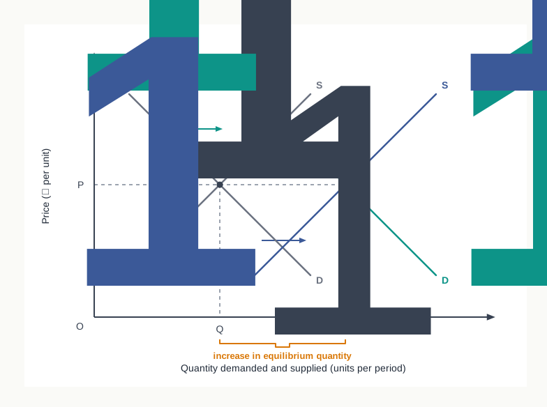
Fig. 6.8 – Demand and supply increasing in the same proportion.
The new equilibrium E1 lies directly to the right of the old equilibrium E. The equilibrium price stays at OP while the equilibrium quantity rises from OQ to OQ1. When demand and supply increase by equal magnitudes, the equilibrium price remains unchanged but the equilibrium quantity increases.
6.5.2 Increase In Demand Greater Than Increase In Supply
Now let both curves shift to the right, but let the demand curve shift further. At the old price the extra quantity buyers want exceeds the extra quantity sellers offer, so an excess demand appears and the price is bid up. The upward pressure coming from demand is only partly offset by the downward pressure coming from supply, and the net effect is a rise in price.
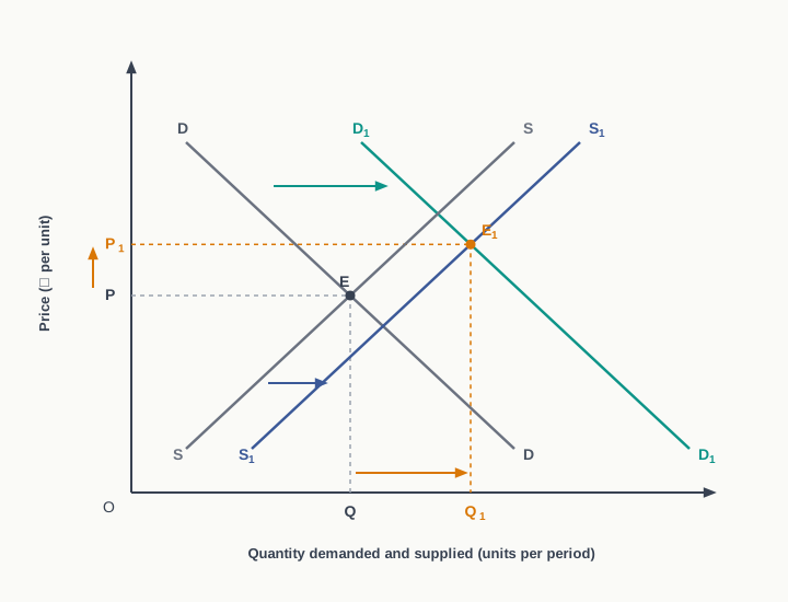
Fig. 6.9 – Increase in demand greater than increase in supply.
Equilibrium moves from E to E1. The equilibrium price rises from OP to OP1 and the equilibrium quantity rises from OQ to OQ1. When the increase in demand is greater than the increase in supply, the equilibrium price rises along with the equilibrium quantity.
6.5.3 Increase In Supply Greater Than Increase In Demand
Reverse the relative sizes of the two shifts. Both curves move to the right, but the supply curve moves further. At the old price the extra quantity offered exceeds the extra quantity wanted, so an excess supply appears and the price is pushed down. The downward pressure from supply outweighs the upward pressure from demand.
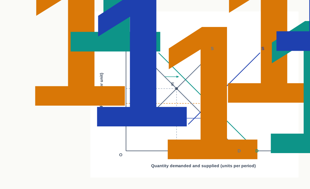
Fig. 6.10 – Increase in supply greater than increase in demand.
Equilibrium moves from E to E1. The equilibrium price falls from OP to OP1 while the equilibrium quantity still rises from OQ to OQ1. When the increase in supply is greater than the increase in demand, the price tends to fall but the equilibrium quantity increases.
The three cases are set out together below.
6.5.4 Simultaneous Decrease In Demand And Supply
The case in which both curves shift to the left needs no new diagram. Read Fig. 6.8 backwards, taking D1D1 and S1S1 as the initial curves and DD and SS as the new ones, and the same reasoning applies with every sign reversed.
A decrease in demand and a decrease in supply both reduce the equilibrium quantity, so here the two work together and the quantity bought and sold must fall. Their effects on price again pull against each other, a decrease in demand pushing the price down and a decrease in supply pushing it up, so three outcomes are possible.
- Decrease in demand equal to decrease in supply — the two pressures cancel, so the equilibrium price is unchanged while the equilibrium quantity falls.
- Decrease in demand greater than decrease in supply — the downward pressure dominates, so the equilibrium price falls and the equilibrium quantity falls.
- Decrease in supply greater than decrease in demand — the upward pressure dominates, so the equilibrium price rises while the equilibrium quantity falls.
The general rule covering all six cases is short. When demand and supply move in the same direction, the effect on quantity is certain and follows that direction, while the effect on price is uncertain and is settled only by the relative magnitudes of the two changes.
6.6 Some Special Cases Of Equilibrium
Every diagram so far has used curves of the normal shape, a demand curve sloping downward and a supply curve sloping upward. Two limiting shapes remain, and they are worth working through because they show, in the sharpest possible form, what decides how an adjustment is divided between price and quantity.
A curve is perfectly elastic when it is a horizontal straight line, parallel to the X-axis: the quantity responds without limit to the slightest change in price. A curve is perfectly inelastic when it is a vertical straight line, parallel to the Y-axis: the quantity does not respond to a change in price at all.
The result in every one of these cases follows from a single idea. An adjustment must show itself somewhere. If one side of the market cannot change its quantity, the whole adjustment falls on price; if one side will not accept any change in price, the whole adjustment falls on quantity.
6.6.1 When The Demand Curve Is Perfectly Elastic Or Perfectly Inelastic
Here the demand curve keeps its limiting shape and the supply curve shifts, as shown in the two panels of Fig. 6.11.
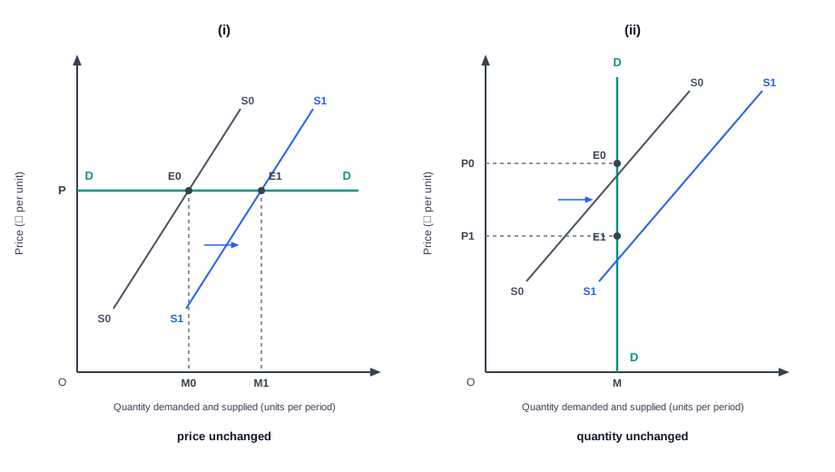
Fig. 6.11 – Change in supply with a limiting demand shape.
When Demand Is Perfectly Elastic
Buyers are willing to take any quantity at the price OP, and nothing at all at any price above it. When supply increases from S0S0 to S1S1, equilibrium slides along the horizontal demand curve from E0 to E1. The quantity bought and sold rises from OM0 to OM1, but the price stays exactly at OP.
The reason lies with the sellers. They cannot charge more than OP, because at any higher price the whole of their market disappears. They have no need to charge less, because at OP they can sell whatever quantity they wish. A change in supply therefore works itself out entirely in quantity.
When Demand Is Perfectly Inelastic
Buyers take the quantity OM whatever the price may be. When supply increases from S0S0 to S1S1, the quantity bought and sold stays at OM and the price falls from OP0 to OP1. A decrease in supply would raise the price in the same way, again without changing the quantity.
Here it is the buyers who leave no room for adjustment. Since they will neither take more when the good becomes cheaper nor less when it becomes dearer, the only thing that can give way is the price.
6.6.2 When The Supply Curve Is Perfectly Elastic Or Perfectly Inelastic
Now the supply curve keeps its limiting shape and the demand curve shifts, as shown in Fig. 6.12.
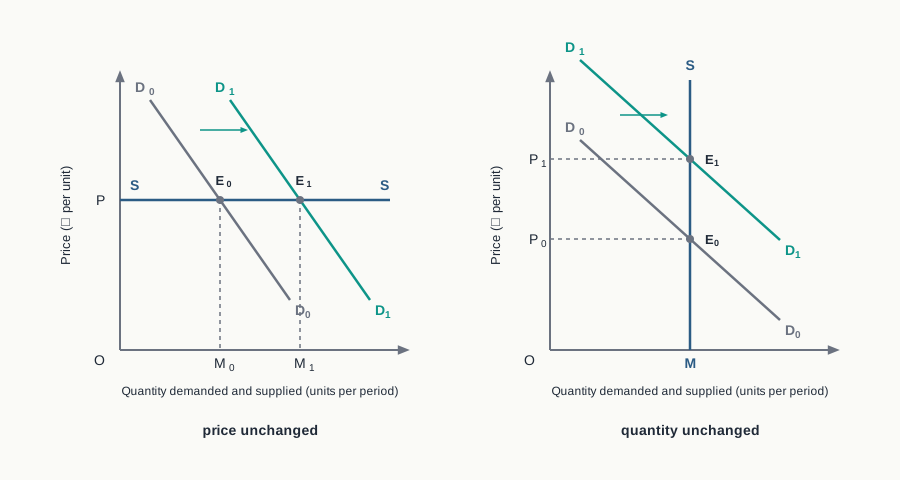
Fig. 6.12 – Change in demand with a limiting supply shape.
When Supply Is Perfectly Elastic
Sellers are willing to supply any quantity at the price OP and none below it, which is the position of an industry able to expand output freely at a constant cost per unit. An increase in demand from D0D0 to D1D1 moves equilibrium along the horizontal supply curve from E0 to E1. The quantity rises from OM0 to OM1 while the price remains OP. Buyers who want more can have as much as they like without bidding the price up.
When Supply Is Perfectly Inelastic
The quantity OM is fixed and cannot be added to, whatever the price. An increase in demand from D0D0 to D1D1 raises the price from OP0 to OP1 and leaves the quantity at OM. Nothing extra reaches the market, so the increase in demand is absorbed wholly by the price.
The four cases can now be collected. Table 6.2 states, for each limiting shape, what happens when the other curve shifts.
Read down the last two columns and a pattern appears. A perfectly elastic curve fixes the price and lets the quantity do all the moving; a perfectly inelastic curve fixes the quantity and lets the price do all the moving. The ordinary cases of Sections 6.3 and 6.4 lie between these two extremes, which is why in them both the price and the quantity change.
6.7 Simple Applications Of Demand And Supply: Price Control
Everything so far has described a free market, one in which the government stands aside and lets the price settle where demand and supply put it. Left to itself the price mechanism does two jobs at once. It clears the market, so that nothing is left unsold and no willing buyer is turned away, and it allocates the commodity, deciding who gets it and how much.
In a mixed economy the government does not always stand aside. It may judge the market outcome to be too harsh on buyers, or too harsh on sellers, and fix the price by law instead. That is price control, and it takes two forms.
- Maximum price legislation, or a price ceiling, which fixes a price above which the commodity may not be sold.
- Minimum price legislation, or a floor price, which fixes a price below which the commodity may not be sold.
The tools of demand and supply are enough to work out what follows in each case, and the answer is the same in both: a legal price that differs from the equilibrium price stops the market from clearing, so some other device has to be found to do the work the price would otherwise have done.
6.7.1 Price Ceiling And Rationing
A government fixes a maximum price when it wants an essential commodity to remain within the reach of poorer buyers. Maximum price limits have been imposed in many countries on food and fuel in times of shortage, and in India on essentials such as foodgrains, sugar and kerosene.
The words ‘to be meaningful’ matter. Fig. 6.13 shows why. If the ceiling is fixed at OP1, above the equilibrium price OP0, it forbids something nobody was doing in any case; the market goes on trading OQ0 at OP0, which remains perfectly legal, and any surplus GH that might appear at OP1 is pushed away by the market itself. A ceiling has an effect only when it is fixed below the equilibrium price.
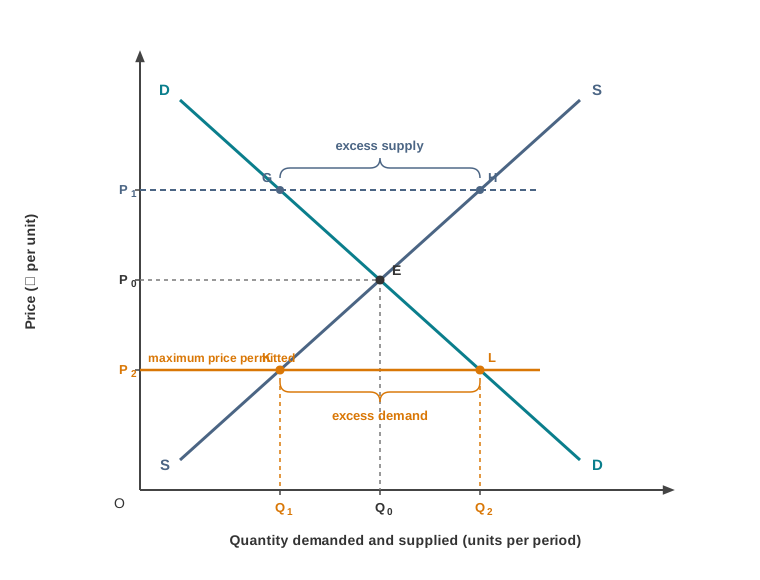
Fig. 6.13 – Price ceiling.
Take the effective case, a ceiling at OP2. The equilibrium price OP0 is now illegal. At OP2 buyers wish to take OQ2 while sellers are willing to offer only OQ1, so an excess demand of OQ1 to OQ2, shown by the distance KL, appears and stays. In a free market this shortage would raise the price and cure itself; here the law forbids the rise, so the shortage becomes a permanent feature of the market. Three consequences follow.
- Effect on price and quantity — buyers pay the lower price OP2, but the quantity actually bought and sold falls from OQ0 to OQ1, because that is all sellers are willing to supply at the controlled price. The policy lowers the price and reduces the amount available at the same time.
- Allocation of the available supply — since the price is not allowed to rise, it can no longer decide who gets the limited quantity, and some other method must be found.
- First come, first served — sellers supply those who arrive first, until the stock runs out. Long queues form, a great deal of time is wasted, and those at the end of the queue may get nothing.
- Allocation by sellers’ preferences — the shopkeeper decides who gets the scarce good, and may keep it for his regular customers.
- Rationing — the government fixes how much each household may buy, which is the method most often adopted.
- Emergence of a black market — some buyers are willing to pay more than the ceiling for extra quantity, and some sellers are willing to sell to them. Since the law forbids such deals, they take place secretly and at prices above the legal price.
Rationing gives every eligible household a claim on part of the scarce supply, which is fairer than leaving the outcome to queues or to the shopkeeper’s favour. It cannot, however, remove the shortage, because it does nothing to increase the quantity produced.
It is a standing comment on human nature that wherever price ceilings and rationing have been introduced, a black market of some sort has appeared alongside them.
6.7.2 Floor Price Or Minimum Support Price
A floor price works in the opposite direction. It is fixed to protect the seller, not the buyer, and it is used where the market price is thought to be too low to give the producer a reasonable return. In India it is applied chiefly to agricultural produce, and the minimum wage laid down for labour is a floor price of the same kind.
Once again the level matters. In Fig. 6.14, a floor fixed at OP1, below the equilibrium price OP0, has no effect whatever: the excess demand GH that would arise at OP1 pushes the price back up to OP0, which is above the floor and therefore lawful. Only a floor above the equilibrium price bites.
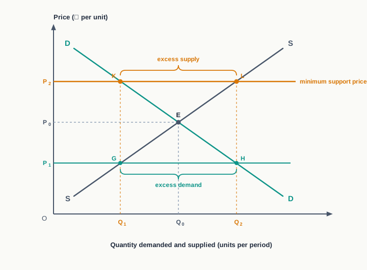
Fig. 6.14 – Floor price.
At the effective floor OP2, sellers wish to offer OQ2 while buyers are willing to take only OQ1. A surplus of OQ1 to OQ2, shown by the distance KL, appears and cannot be cleared, because the price is not allowed to fall. Its consequences are these.
- Producers get a higher price, but sell less — the price is OP2 instead of OP0, yet the quantity actually bought and sold falls to OQ1, which is smaller than the equilibrium quantity OQ0. A producer who cannot dispose of his stock at the legal price may be tempted to break the law and sell below it.
- The government has to buy the surplus — if the floor price is to hold, someone must take the unsold quantity off the market at that price, and it is the government that does so. The stock accumulated in this way is called a buffer stock, and it can be released later when supplies are short.
- The policy is costly — the purchases have to be paid for out of public revenue, and the stock has to be stored, guarded and eventually disposed of, some of it deteriorating in the meantime.
6.7.3 Price Ceiling And Floor Price Compared
The two policies are mirror images of each other, and the differences between them are set out below.
Both policies come to the same general conclusion. A legal price fixed away from the equilibrium price prevents the market from clearing, and the gap it creates does not go away by itself. Something must then be put in the place of the price to decide who gets the good or who is left with the surplus, whether that is a ration card, a queue, a black market or a government purchase. This is the cost that has to be weighed against whatever the control was meant to achieve.
6.8 Summary
- Equilibrium is a state of balance between two opposing forces, from which there is no tendency to change unless one of the forces influencing the balance itself changes.
- In a market the opposing forces are demand and supply. The market is in equilibrium when the quantity demanded of a commodity equals the quantity supplied of it, and in disequilibrium when the two are unequal.
- The price cannot settle anywhere at all. Marginal utility fixes the highest price a buyer can be induced to pay and marginal cost fixes the lowest price a seller can be induced to accept, so the agreed price lies between the two limits.
- Equilibrium price is the price at which quantity demanded equals quantity supplied. At that price the market is cleared, and neither side has any incentive to change its behaviour.
- Equilibrium quantity is the amount actually bought and sold at the equilibrium price, the quantity demanded and the quantity supplied being equal there.
- In a demand and supply schedule the two quantities are equal at one price only. That price is the equilibrium price and every other price in the schedule is a disequilibrium price.
- Disequilibrium takes two forms, and each corrects itself.
- Excess demand is the amount by which quantity demanded exceeds quantity supplied. It arises below the equilibrium price, appears as a shortage, and competition among buyers pushes the price up.
- Excess supply is the amount by which quantity supplied exceeds quantity demanded. It arises above the equilibrium price, appears as a surplus, and competition among sellers pushes the price down.
- Diagrammatically, equilibrium price and equilibrium quantity are determined at the point where the downward-sloping demand curve intersects the upward-sloping supply curve, which is the only point lying on both.
- A stable equilibrium is one which, if displaced by some small disturbance, brings into operation forces that restore the initial equilibrium position.
- Neither demand alone nor supply alone determines price. Marshall compared the two to the blades of a scissors, both being necessary to the cut.
- An increase in demand raises both the equilibrium price and the equilibrium quantity; a decrease in demand lowers both. The adjustment takes place as a movement along the unchanged supply curve.
- An increase in supply lowers the equilibrium price and raises the equilibrium quantity; a decrease in supply raises the price and lowers the quantity. The adjustment takes place as a movement along the unchanged demand curve.
- When demand and supply change together in the same direction, the effect on quantity is certain and follows that direction, while the effect on price depends on the relative magnitudes of the two changes.
- If the two increase equally, the equilibrium price is unchanged and the equilibrium quantity rises.
- If the increase in demand is greater, both the equilibrium price and the equilibrium quantity rise.
- If the increase in supply is greater, the equilibrium price falls while the equilibrium quantity rises.
- When both demand and supply decrease, the equilibrium quantity must fall, and the equilibrium price remains unchanged, falls or rises according as the decrease in demand is equal to, greater than or smaller than the decrease in supply.
- Where one curve takes a limiting shape, the adjustment falls wholly on one side. A perfectly elastic curve, drawn parallel to the X-axis, holds the price unchanged and lets the quantity change; a perfectly inelastic curve, drawn parallel to the Y-axis, holds the quantity unchanged and lets the price change.
- A price ceiling is the maximum legal price a seller may charge. To be effective it must be fixed below the equilibrium price, and it then creates a lasting shortage, reduces the quantity actually sold, has to be accompanied by rationing, and tends to give rise to a black market.
- A floor price, or minimum support price, is the minimum legal price below which a seller may not sell. To be effective it must be fixed above the equilibrium price, and it then creates a surplus which the government generally purchases and holds as a buffer stock.
- Any legal price fixed away from the equilibrium price prevents the market from clearing, so some other device — a ration card, a queue, a black market or a government purchase — has to do the work that the price would otherwise have done.
The four single shifts studied in this chapter are collected below.
6.9 Points to Ponder
- A free price rations a scarce good by giving it to whoever is willing to pay most, while a ration card rations it by entitlement but cannot bring a single extra unit into existence. If a country faced a serious shortage of foodgrains for one season and had to choose between the two methods, on what grounds should the choice be made, and what would be lost either way?
- The government supports the price at which the farmer sells his grain and holds down the price at which the poor household buys it, so the same grain has a high floor at one end of the chain and a low ceiling at the other. Who bears the difference between the two prices, and for how long can such an arrangement be carried?
- A bumper harvest increases supply, lowers the price and raises the quantity sold. Yet where demand for the crop is inelastic, growers as a body may end the season with smaller earnings than in an ordinary year. Is a bumper harvest then good for the farmer, and what, if anything, should policy do about a good year?
- The model treats equilibrium as stable, so that a market displaced from it comes back. But a farmer decides how much to sow by looking at last year’s price, and a high price this year may produce a glut and a crash next year. Are there markets in which the forces of adjustment carry the price past equilibrium rather than to it?
- The supply of land in a city centre is fixed, so a rise in demand raises its price without adding one square metre to what is available. The owner has produced nothing extra, yet his wealth has grown. Where does that gain come from, and is there a case for treating it differently from income earned by producing something?
- A demand curve records only those wants that are backed by the ability to pay, so a household too poor to buy never appears on it at all. If the market clears at the equilibrium price while such households go without, in what sense can that outcome be called a satisfactory one?
6.10 Objective Questions
- At any price above the equilibrium price, a competitive market will experience: [1]
- excess demand, and the price will rise
- excess supply, and the price will fall
- excess demand, and the price will fall
- neither excess demand nor excess supply
- Assertion (A): An increase in the supply of a commodity lowers its equilibrium price and raises its equilibrium quantity. [1] Reason (R): A rightward shift of the supply curve creates an excess supply at the price that was ruling earlier.
- Both A and R are true, and R is the correct explanation of A.
- Both A and R are true, but R is not the correct explanation of A.
- A is true, but R is false.
- A is false, but R is true.
- A price ceiling affects the market only when it is fixed ______ the equilibrium price. [1]
- State whether the following statement is true or false: when demand and supply both increase in the same proportion, the equilibrium quantity remains unchanged. [1]
- Match each item in Column I with the correct item in Column II. [1]
| Column I | Column II |
|---|---|
| a. Perfectly inelastic supply | i. A change in supply leaves the equilibrium price unchanged |
| b. Perfectly elastic demand | ii. A specified quantity is distributed at a price fixed by the government |
| c. Rationing | iii. A change in demand leaves the equilibrium quantity unchanged |
6.11 Check Your Concepts
- Distinguish between excess demand and excess supply. [2]
- Explain what happens in a market when the prevailing price is below the equilibrium price. [3]
- With the help of a diagram, show the effect on equilibrium price and equilibrium quantity of a sharp rise in the price of an important raw material used in making a commodity. [4]
- Why may the equilibrium price of a commodity remain unchanged even though both its demand and its supply have increased? Explain with the help of a diagram, and state what happens to the equilibrium quantity in this case. [6]
6.12 Case-Based Question
- During the pilgrimage season the price of packaged drinking water in a hill district rises steeply, and the state government fixes a maximum price of ₹15 a bottle, well below the price at which the market had been clearing. Vimal Traders, one of the largest suppliers in the district, finds that its stock is exhausted by the middle of every morning, and shopkeepers begin keeping bottles aside for their regular customers.
- Using the tools of demand and supply, explain why the shops run out of stock every day at the controlled price. [2]
- Suggest one measure the government could adopt to distribute the limited supply among buyers, and state one drawback of that measure. [2]