Chapter 7: Production and the Laws of Returns
A knitwear unit in Tiruppur owns twelve stitching machines. Orders rise, but new machines take months to arrive and install, so the owner does the only thing possible in the meantime — puts on more workers. Output climbs, then climbs more slowly, and past a point the shop floor is so crowded that another pair of hands adds almost nothing. That small story contains the whole of this chapter. A firm’s output depends on the inputs it uses, and the relation between the two is the production function. What a firm can vary depends on how much time it has: in the short run some factors are fixed, in the long run none are. When only one factor can be varied, output responds according to the law of variable proportions; when every factor is changed together, output responds according to returns to scale. The chapter explains production and the production function, builds the total, average and marginal product measures and the relations between them, works through the three stages of production, and compares returns to a factor with returns to scale.
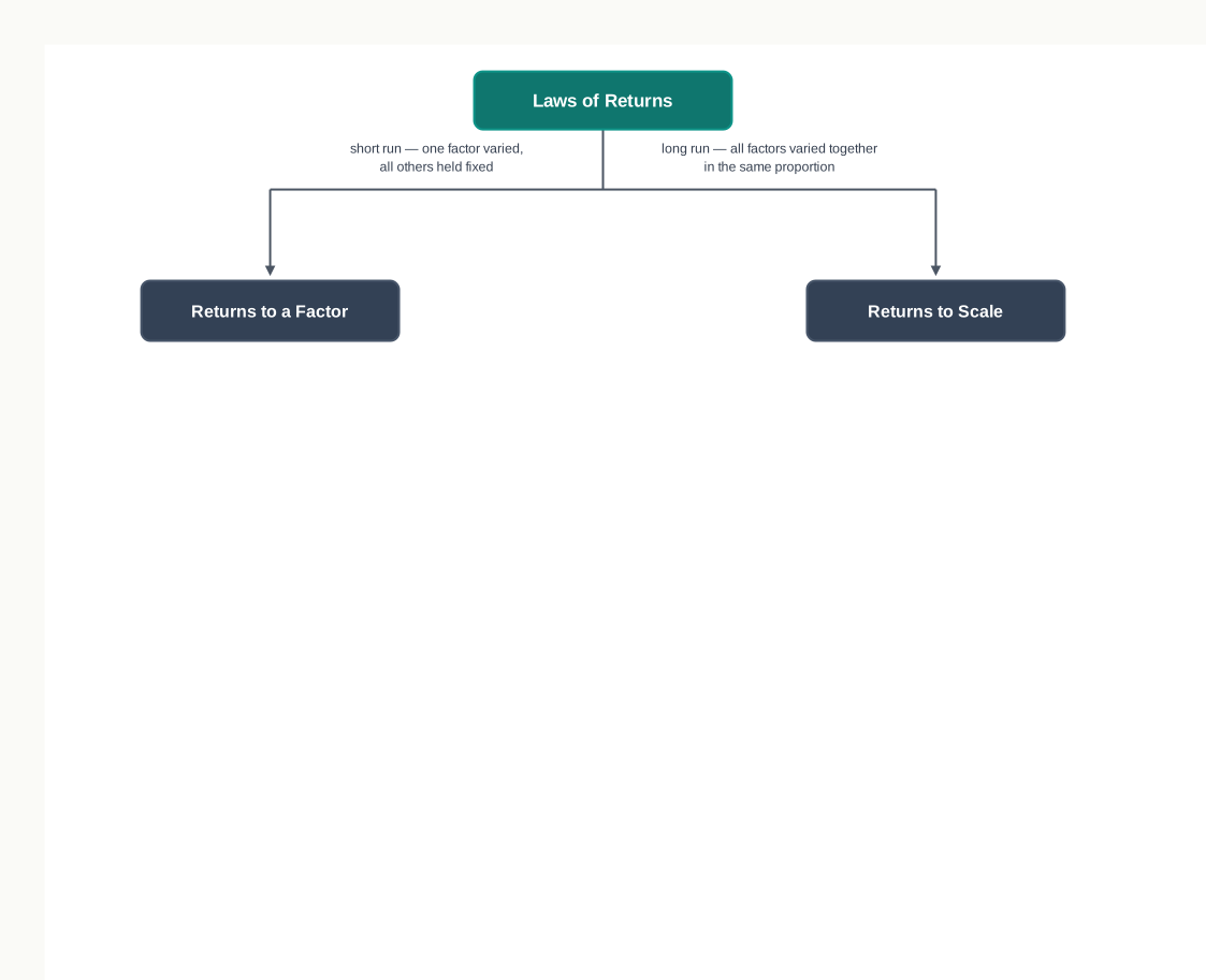
Fig. 7.0 – The laws of returns at a glance.
7.1 The Concept of Production
Every firm faces a smaller version of the constraint the whole economy faces. It has a limited quantity of land, labour, capital and enterprise at its disposal, and it must turn that limited bundle into goods and services people are willing to buy. How much output a given bundle of resources will yield is therefore not a technical curiosity. It is the question a producer must answer before deciding how much to supply and at what price.
The study of the relation between inputs and output is called the theory of production. The study of the relation between output and the cost of producing it is called the theory of cost. The first provides the base for the second, because the cost of any level of output depends on the physical quantities of inputs that level requires and on the prices of those inputs. If input prices are taken as given, cost depends entirely on the physical relation between inputs and output. This chapter deals with that physical relation; the next takes up cost.
7.1.1 Production as the Creation of Utility
In everyday speech, production means making something. Cloth is produced in a textile mill by combining yarn, dyes, chemicals and labour, and the word is reserved for the physical conversion of raw material into a tangible good. This is a narrow view, and economics does not use it.
Economists define production more widely as any activity that creates utility — the capacity of a good or a service to satisfy a human want. A thing is produced when it is made useful, whether or not anything tangible has come into existence.
Two consequences follow, and both matter for the way national output is counted later in the course.
- Production does not create matter — a producer only changes the form of what already exists, or the place at which it is available, or the time at which it is available. Spinning cotton into yarn changes its form; moving grain from a surplus State to a deficit one changes its place; storing it from harvest to the lean season changes the time at which it can be used. Each act adds utility, so each is production.
- Production is not confined to goods — the services of a doctor, a teacher, a lawyer, a barber or a musician satisfy wants exactly as material goods do, so rendering a service is production in the same sense as making a good.
Trading and transport are production for the same reason. A good sitting in a factory warehouse cannot satisfy anyone’s want; production is not complete until the good has actually reached the consumer, and the trader and the carrier are the ones who complete it.
7.1.2 Inputs, Output and the Producer’s Problem
The resources a firm uses in production are called inputs, or factors of production — land, labour, capital and enterprise, together with the raw materials and services bought in from other firms. What emerges from the process is the output, the quantity of the good or service produced.
Both are measured as flows, that is, as quantities per period of time. It means nothing to say that a unit uses forty workers and produces eight hundred shirts unless the period is stated; forty workers a day producing eight hundred shirts a day describes a rate of production, and it is rates that a producer plans with. The relation between the two flows is set out in Fig. 7.1.
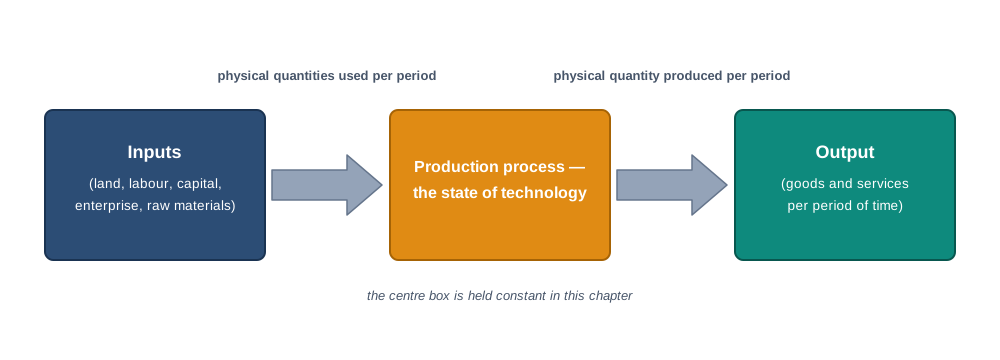
Fig. 7.1 – Inputs, the production process and output.
Once inputs and output are set out this way, the producer’s problem separates into two questions. The first is technical: what is the largest output the firm can get from a given bundle of inputs, given the technology available to it? The second is economic: of the input combinations that can yield the output the firm wants, which is the cheapest at the prices it must pay?
This chapter answers the first question and leaves the second to the theory of cost. Technology is therefore held constant throughout, and the only thing allowed to change is the quantity of inputs. Even that change can happen in two quite different ways — one input may be varied while the rest are held fixed, or every input may be varied together. The two cases behave so differently that economics gives them separate names, returns to a factor and returns to scale, and the rest of the chapter takes them in turn.
7.2 The Production Function
A producer who wants to plan output needs more than a list of the inputs available. The producer needs to know how much output each combination of those inputs will actually yield, because that is what fixes how much of each input to buy and, once input prices are known, what the output will cost. Economics sets out that information in a single relation called the production function.
7.2.1 Meaning of the Production Function
The production function is the functional relation between the physical quantities of inputs used and the physical quantity of output obtained, given the state of technology. It is a statement of what is technically possible, and not of what is profitable.
Two features of the definition need care. First, the function shows the maximum quantity of output obtainable from a given quantity of inputs, on the assumption that the best technique available is used and that nothing is wasted. Second, it can be read the other way round with equal sense: it shows the minimum quantity of inputs needed to produce a given quantity of output. A production function for a shoemaking unit tells us either the largest number of pairs that can be turned out per day from given quantities of leather, glue, machinery and labour, or the smallest quantities of those inputs needed to turn out, say, a hundred pairs a day.
A production function may be presented as a table, as a graph or as an algebraic equation. In its most general algebraic form it says that the output of a commodity depends on the physical quantities of all the inputs used to produce it.
\[Q_X = f(f_1, f_2, \ldots, f_n)\]
Here \(Q_X\) is the quantity of output of commodity X produced per period of time, measured in physical units such as pens or metres of cloth, and \(f_1, f_2, \ldots, f_n\) are the physical quantities of the different inputs used, each measured in its own physical unit. \(Q_X\) is the dependent variable and the inputs are the independent variables. The equation is read as: output depends on, and is determined by, the quantities of inputs employed.
Economic analysis usually simplifies this to two inputs, labour and capital, because two are enough to show everything the theory needs to show.
\[Q_X = f(L, K)\]
Here \(L\) is the quantity of labour employed per period, measured in workers or worker-hours, and \(K\) is the quantity of capital employed per period, measured in machines or machine-hours. The equation is read as: the output of commodity X depends on the quantities of labour and capital used to produce it.
7.2.2 Features of the Production Function
The following features follow from the definition and should be stated whenever the concept is explained.
- It relates to a period of time — inputs and output are both flows, so a production function is always expressed per day, per month or per year. A statement of quantities without a period is meaningless.
- It is a physical relation — both inputs and output are expressed in physical units and not in money. Prices enter the analysis only later, when the theory of cost is taken up.
- It is a purely technological relation — what can be produced from a given bundle of inputs depends on the state of technology. A change in technique gives a new and different production function, so technology is held constant while one production function is being discussed.
- It assumes technical efficiency — the output shown is the largest obtainable, so every point on the function assumes that no input is being wasted.
7.2.3 The Short Run and the Long Run
Whether a firm can vary an input at all depends on how much time it has. A unit that receives a large order this week cannot conjure up a second factory building by Friday, but it can call in extra workers and buy more raw material. Economics therefore divides time not by the calendar but by what the firm is free to change, and distinguishes two periods.
Inputs that cannot be varied within the period under consideration are called fixed factors — plant, machinery, factory buildings, the services of the entrepreneur. Inputs whose quantity can be varied within that period are called variable factors — labour, raw material, power.
In the short run, then, the size of the plant is given. An increase in output has to be squeezed out of that plant by working it more intensively — more workers on the same machines, more shifts, more raw material — and this is why the short run is described as the fixed-plant period.
A firm in the long run can install new machinery, build a new shed or set up an entirely new plant, and can equally scrap capacity it no longer wants. Every input is variable, so output can be expanded or contracted by changing the scale of the whole operation rather than by working a given plant harder.
The distinction does not correspond to any fixed stretch of calendar time. What counts is how long the firm needs to adjust its plant, and that differs sharply from one industry to another.
7.2.4 Short-Run and Long-Run Production Functions
Corresponding to the two periods there are two production functions, and the whole of this chapter is built on the difference between them.
A short-run production function refers to a situation in which only one input is variable and all other inputs are held constant. If capital is fixed at a given number of machines and labour alone is varied, the function reduces to \(Q_X = f(L)\), output depending on labour alone. Because one factor is being changed while the others stay put, the proportion in which the factors are combined changes as output changes. The behaviour of output under these conditions is called returns to a factor, and it is the subject matter of the law of variable proportions taken up in Section 7.5.
A long-run production function refers to a situation in which all inputs are variable. When every input is increased or decreased simultaneously and in the same proportion, the factor proportions stay exactly as they were and what changes is the scale of production. The behaviour of output under these conditions is called returns to scale, taken up in Section 7.6.
The main points of difference between the two are set out below.
7.3 Total, Average and Marginal Physical Products
In the short run the size of the plant is given, so the only way a firm can change its output is by changing the quantity of the variable factor applied to that plant. The question this raises is a question of measurement: as more of the variable factor is put to work, by how much does output change? Economics answers it with three measures — total product, average product and marginal product — which are three ways of looking at the same set of figures.
Throughout this section we take a small printing press that owns four printing machines. The machines are the fixed factor, labour is the variable factor, and output is the number of booklets printed per day. The schedule of output as more workers are employed is given in Table 7.1, and every relationship in this section can be read off it.
7.3.1 Total Physical Product
Total product, or total physical product, is the total quantity of output produced during a given period of time by combining a particular quantity of the variable factor with the given quantity of the fixed factor. It is also called total returns.
Column 2 of Table 7.1 traces total product as labour increases. Two things about it are worth noticing at once. Total product rises as workers are added, but it does not rise for ever: it reaches a maximum of 280 booklets and then falls. And it does not rise at a steady rate: the second worker adds 50 booklets to output while the sixth adds only 30. It is this uneven behaviour that the remaining two measures are designed to capture.
7.3.2 Average Physical Product
Average product, or average physical product, is the output per unit of the variable factor. It answers the question of how productive each worker is on average, once the whole output is shared out over the workers employed. It is also called average returns.
\[AP_L = \dfrac{TP_L}{L}\]
Here \(AP_L\) is the average product of labour, \(TP_L\) is the total product of labour and \(L\) is the number of units of labour employed. Both \(TP_L\) and \(AP_L\) are measured in units of output per period, and \(AP_L\) is read as output per worker per period.
Column 3 of Table 7.1 is column 2 divided by column 1. When three workers produce 150 booklets, average product is 50 booklets per worker. Average product rises as the first few workers are added, reaches a maximum of 50 booklets at the fourth worker, and falls thereafter.
7.3.3 Marginal Physical Product
Marginal product, or marginal physical product, is the addition made to total product when one more unit of the variable factor is employed, the quantity of the fixed factor remaining unchanged. It is also called marginal returns. Where average product describes the whole workforce, marginal product isolates the contribution of the last worker taken on, and it is therefore the measure a producer deciding whether to hire one more hand actually needs.
\[MP_L = \dfrac{\Delta TP}{\Delta L}\]
Here \(MP_L\) is the marginal product of labour, \(\Delta TP\) is the change in total product and \(\Delta L\) is the change in the quantity of labour employed. The result is measured in units of output per additional worker. Where labour increases one unit at a time, the formula reduces to a subtraction.
\[MP_n = TP_n - TP_{n-1}\]
Here \(MP_n\) is the marginal product of the \(n\)th unit of the variable factor, \(TP_n\) is total product when \(n\) units are employed and \(TP_{n-1}\) is total product when one unit less is employed. Reading column 4 of Table 7.1 this way, the third worker’s marginal product is \(150 - 90 = 60\) booklets.
Marginal product rises to a maximum of 60 booklets at the third worker, falls thereafter, becomes zero at the eighth worker and turns negative at the ninth.
7.3.4 Deriving One Measure from Another
The three measures are not independent pieces of information. Given any one of them, the other two can be worked out, and an examiner may ask for exactly that.
- Total product from marginal products — since each unit’s marginal product is its addition to total output, total product is the sum of the marginal products of all units employed. Thus \(TP = \Sigma MP\), and in Table 7.1 the total product of three workers is \(40 + 50 + 60 = 150\) booklets.
- Total product from average product — total product is average product multiplied by the number of units of the variable factor, so \(TP = AP \times L\). In Table 7.1, four workers with an average product of 50 booklets give a total product of 200 booklets.
- Average product from total product — average product is total product divided by the units of the variable factor employed.
- Marginal product from total product — marginal product is the difference between successive totals.
7.3.5 Relationship between Total Product and Marginal Product
Marginal product is the rate at which total product changes, so the shape of the total product curve and the height of the marginal product curve are two statements of one fact. The relationship has four parts, each of which can be checked against Table 7.1 and seen in Fig. 7.2.
- When total product increases at an increasing rate, marginal product rises. In Table 7.1 this holds up to the third worker, where marginal product climbs from 40 to 60 booklets.
- When total product increases at a diminishing rate, marginal product falls but stays positive. This holds from the fourth worker to the seventh, where marginal product falls from 50 to 10 booklets while output is still rising.
- When total product is at its maximum, marginal product is zero. In the table this happens at the eighth worker, where output stands at its peak of 280 booklets and the eighth worker adds nothing.
- When total product begins to fall, marginal product becomes negative. The ninth worker reduces output to 270 booklets, so marginal product is \(-10\).
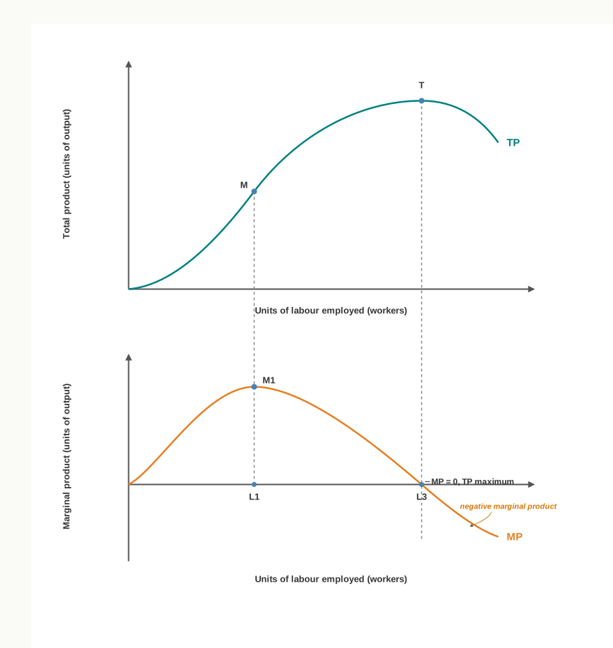
Fig. 7.2 – Total product and marginal product curves.
7.3.6 Relationship between Average Product and Marginal Product
The relationship between the two is the ordinary arithmetic of averages. An average rises when a new item added to it is larger than the existing average, and falls when the new item is smaller. Marginal product is the new item and average product is the average, so the following must hold, as Fig. 7.3 shows.
- When marginal product is greater than average product, average product rises. In Table 7.1 this holds up to the fourth worker. The sense of it is plain: if an extra worker is to raise the productivity of the whole workforce, that worker’s own contribution must exceed what the existing workers were averaging.
- When marginal product equals average product, average product is at its maximum. In Table 7.1 this happens at the fourth worker, where both stand at 50 booklets.
- When marginal product is less than average product, average product falls. This holds from the fifth worker onwards, where marginal product of 40 booklets pulls the average down from 50 to 48.
- Marginal product may be positive, zero or negative, but average product is always positive so long as any output is being produced, because a positive total divided by a positive number of workers cannot be negative.
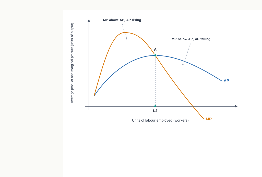
Fig. 7.3 – Average product and marginal product curves.
7.4 Returns to a Factor
Total, average and marginal product tell us what output does. The next step is to name the possibilities. When a producer keeps the plant unchanged and goes on adding units of a single variable factor, the extra output obtained from each successive unit may rise, may stay the same, or may fall. These three possibilities are what economics calls returns to a factor, and the whole of short-run production theory is built on the order in which they occur.
7.4.1 Meaning of Returns to a Factor
Returns to a factor means the change in the physical output of a good when the quantity of one factor is increased while the quantities of all other factors are held constant.
Two features of this definition should be fixed firmly in mind, because every distinction later in the chapter turns on them. Returns to a factor is a short-run idea, since it presupposes that some factors are fixed and cannot be varied at all. And it necessarily involves a change in factor proportions: if four printing machines are worked first by two workers and then by three, the ratio in which capital and labour are combined has changed, and it is this changed proportion, not the extra worker by himself, that explains the new level of output.
Returns to a factor is measured by what happens to marginal product. That is the natural measure, because marginal product isolates the contribution of the additional unit of the variable factor, which is precisely what the concept asks about.
7.4.2 Increasing Returns to a Factor
Increasing returns to a factor refers to a situation in which each additional unit of the variable factor, combined with the given fixed factor, adds more to total output than the unit before it. In other words, the marginal product of the variable factor rises as more of it is used, and total product therefore increases at an increasing rate.
This is the position in Table 7.1 up to the third worker, where marginal product climbs from 40 to 50 and then to 60 booklets. Output is not merely rising; it is rising faster with every worker taken on.
7.4.3 Constant Returns to a Factor
Constant returns to a factor refers to a situation in which each additional unit of the variable factor adds the same amount to total output as the unit before it. Marginal product is constant, so total product increases at a constant rate.
Constant returns is the intermediate case between the other two. Increasing returns do not turn abruptly into diminishing returns; there is usually a short range over which the fixed factor has come to be used at about its ideal ratio with the variable factor, and over that range the marginal product of the variable factor holds steady at its highest level before it begins to fall. In Table 7.1 the schedule moves straight from rising to falling marginal product, so no constant stretch appears there, but the possibility is real and must be stated whenever the three kinds of returns are listed.
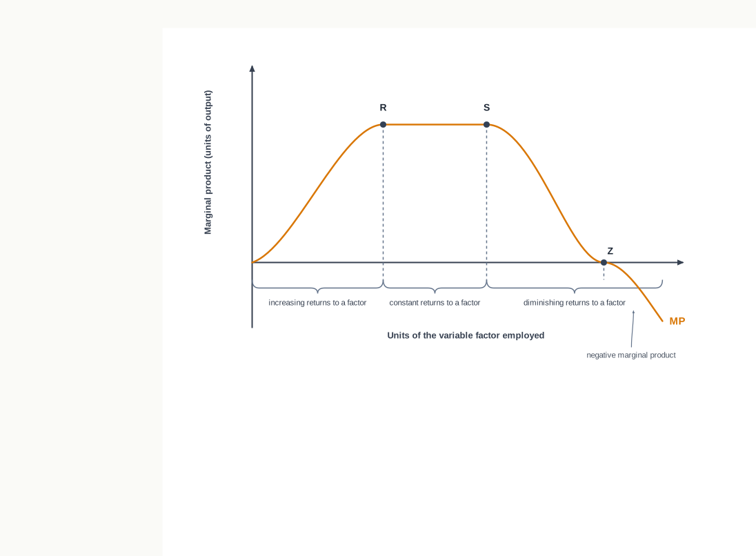
Fig. 7.4 – The three kinds of returns to a factor.
7.4.4 Diminishing Returns to a Factor
Diminishing returns to a factor refers to a situation in which each additional unit of the variable factor adds less to total output than the unit before it. Marginal product falls as more of the variable factor is used, so total product goes on increasing but at a diminishing rate.
In Table 7.1 this begins with the fourth worker and continues to the seventh, marginal product falling from 50 to 10 booklets. Output is still climbing throughout — it reaches its peak of 280 booklets — but each worker is contributing less than the last. Pushed far enough, the process ends in a marginal product of zero at the eighth worker and a negative marginal product at the ninth, at which point total product itself begins to fall.
Earlier economists, Marshall among them, set these three possibilities out as three separate laws — the law of increasing returns, the law of constant returns and the law of diminishing returns — and held that adding a variable factor to a fixed factor leads first to increasing returns and ultimately to diminishing returns, with constant returns as the stage between. Modern treatment draws the three together into a single statement, the law of variable proportions, which is taken up next.
7.5 The Law of Variable Proportions
Section 7.4 named three possible kinds of returns to a factor but said nothing about the order in which a producer meets them. That order is not arbitrary. As a variable factor is added to a fixed factor, returns behave in a regular sequence, and the generalisation that states this sequence is the law of variable proportions.
The name explains itself. When different quantities of a variable factor are applied to an unchanged quantity of a fixed factor, the proportion in which the two are combined keeps changing. In the printing press of Table 7.1 one worker to four machines is a ratio of 4K : 1L; a second worker makes it 4K : 2L; a third, 4K : 3L. Since output responds to these changing proportions, the law that describes the response is named after them. The law is an extension of what classical economists called the law of diminishing returns.
7.5.1 Statement of the Law
The law can be stated in terms of any of the three measures, and the three statements say the same thing. In terms of total product, output rises first at an increasing rate and then at a diminishing rate. In terms of marginal product, the marginal product of the variable factor rises at first, reaches a maximum and then falls. In terms of average product, the average product of the variable factor rises at first, reaches a maximum and then falls.
The word ‘eventually’ is the heart of the law. It does not claim that returns diminish from the very first unit; it claims that whatever happens early on, diminishing returns must set in at some point, because the fixed factor cannot be stretched indefinitely.
7.5.2 Assumptions of the Law
The law holds only under certain conditions, and each condition has a reason.
- The state of technology is given and unchanged — an improvement in technique would raise output at every level of the variable factor, so any fall in marginal product could be offset by better technology and the law would not be observable.
- Some factors are fixed while others are varied — the law describes a short-run situation. If every factor could be varied, factor proportions would not change and the question the law answers would not arise.
- Factor proportions can be altered — the law does not apply where the factors must be combined in a rigid technical ratio, since in that case an extra unit of one factor alone simply cannot be put to work.
- All units of the variable factor are homogeneous and equally efficient — otherwise a fall in marginal product might be explained by later workers being less able than earlier ones, rather than by the changing proportion between the factors.
7.5.3 Illustration of the Law
Table 7.1 illustrates the law numerically. Four printing machines are the fixed factor, and labour is increased from one worker to nine.
Up to the third worker, total product rises at an increasing rate and marginal product climbs from 40 to 60 booklets. Rising marginal product pulls average product up with it. Beyond the third worker the rate of increase in total product switches from increasing to diminishing, and marginal product begins to fall, though it remains positive; average product goes on rising for one worker more and reaches its maximum of 50 booklets at the fourth worker, where marginal product has fallen to exactly the level of average product. From the fifth worker onwards falling marginal product drags average product down as well. Total product reaches its maximum of 280 booklets at the eighth worker, where marginal product is zero. Employing a ninth worker is worse than useless: marginal product turns negative and total product falls to 270 booklets.
7.5.4 The Three Stages of Production
The behaviour of total, average and marginal product as the variable factor is increased is conventionally divided into three stages. Fig. 7.5 shows them, with the upper panel carrying the total product curve and the lower panel the average and marginal product curves drawn on the same scale of the variable factor.
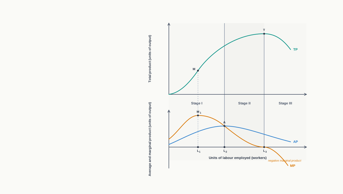
Fig. 7.5 – The three stages of production.
7.5.4.1 Stage I — Increasing Returns
The first stage runs from the origin to the point at which average product is at its maximum, point A in Fig. 7.5, corresponding to the fourth worker in Table 7.1.
Throughout this stage total product increases: at an increasing rate up to the point of inflexion M, and at a diminishing rate between M and A. The point M, where the total product curve changes the direction of its curvature, is called the point of inflexion, and marginal product is at its maximum there. Marginal product rises to that maximum and then falls, but stays positive throughout the stage. Average product rises throughout and ends the stage at its highest level, with marginal product equal to it.
Some economists prefer to end the first stage at M, where marginal product is maximum, rather than at A. The essential character of the stage is the same on either view.
7.5.4.2 Stage II — Diminishing Returns
The second stage runs from the point of maximum average product to the point at which marginal product becomes zero — from A to T in Fig. 7.5, and from the fourth worker to the eighth in Table 7.1.
Total product continues to increase throughout this stage, but at a diminishing rate, and reaches its maximum at the end of the stage. Both average product and marginal product are falling, yet both remain positive, with marginal product ending the stage at zero.
7.5.4.3 Stage III — Negative Returns
The third stage begins beyond the point of maximum total product, that is, beyond the eighth worker in Table 7.1.
Total product falls, so the total product curve slopes downward. Marginal product is negative and the marginal product curve lies below the X-axis. Average product continues to fall but stays positive, since a positive output divided by a positive number of workers can never be negative.
The three stages are summarised in Table 7.2.
7.5.5 Reasons behind the Three Stages
A law is worth little unless the reasons for it are understood. The three stages arise from the changing relation between the fixed factor and the variable factor.
Causes Of Increasing Returns
- Fuller utilisation of the fixed factor — fixed factors are indivisible, that is, they cannot be bought or used in fractions to suit the level of output. Four printing machines must be installed whole, so when very few workers are employed part of that capacity stands idle. Each additional worker brings the fixed factor closer to full use, and output rises more than in proportion.
- Increase in the efficiency of the variable factor — as the number of workers rises, the work can be divided among them according to skill and aptitude. Division of labour and specialisation raise the efficiency of the variable factor itself, and marginal product rises accordingly.
Causes Of Diminishing Returns
- Disturbance of the optimum proportion — there is one combination at which the fixed factor is used fully and efficiently. Once that combination is reached, every further unit of the variable factor pushes the proportion away from the optimum, and average and marginal product fall.
- Imperfect substitutability of the factors — factors of production are only imperfect substitutes for one another. Labour can be put in the place of capital up to a point, but beyond that point no quantity of labour can do the work of a machine that is not there, so returns must diminish.
Causes Of Negative Returns
- Overcrowding of the fixed factor — too many workers on the given fixed factor means less equipment available to each, and workers begin to obstruct one another. Productivity falls far enough for total output to decline.
- Problems of management — a workforce too large for the plant becomes difficult to supervise. Responsibility is shifted from one worker to another, accountability is hard to fix, and efficiency falls.
7.5.6 The Stage in Which a Producer Operates
Given the three stages, in which of them will a rational producer choose to operate? The answer is reached by eliminating the other two.
No producer will operate in Stage III. Here marginal product is negative, so the producer can raise total output by employing fewer units of the variable factor. Even if labour were available free of charge, employing more of it in this stage would reduce output. Stage III is therefore sometimes called the stage of economic absurdity.
No producer will stop within Stage I either. Throughout this stage the average product of the variable factor is still rising, which means the average cost of producing a unit of output is still falling. A producer who halts before the end of Stage I is giving up gains that are there for the taking, and no rational producer stops while profits are still increasing with output.
By elimination, a rational producer operates in Stage II. This is the stage in which total product is at its highest levels and both average and marginal product are positive though falling. Exactly where within Stage II the producer settles depends on the prices of the factors of production, which belong to the theory of cost rather than to the theory of production.
7.6 Returns to Scale
Everything so far has assumed that the plant is given. Once we move to the long run that assumption goes: no factor is fixed, and the firm can change the size of its whole operation. The question then becomes a different one. Instead of asking what happens when one factor is added to an unchanged plant, we ask what happens when every factor is increased together.
7.6.1 Meaning of Returns to Scale
When all inputs are changed simultaneously and in the same proportion, what changes is the scale of production. Factor proportions stay exactly as they were — doubling both labour and capital leaves the ratio between them untouched — so whatever happens to output cannot be attributed to a changed combination of factors. It is the size of the operation, and nothing else, that has altered.
7.6.2 Increasing, Constant and Diminishing Returns to Scale
Output may respond to a change in scale in three ways, and the three are distinguished by comparing the proportionate change in output with the proportionate change in inputs. Table 7.3 sets out an illustration of each.
- Increasing returns to scale — output increases more than in proportion to the increase in inputs. In Table 7.3 a doubling of both inputs raises output from 100 to 250 units, an increase of 150 per cent against an increase of 100 per cent in inputs.
- Constant returns to scale — output increases exactly in proportion to the increase in inputs. Doubling both inputs doubles output from 100 to 200 units.
- Diminishing returns to scale — output increases less than in proportion to the increase in inputs. Doubling both inputs raises output from 100 to only 150 units, an increase of 50 per cent against an increase of 100 per cent in inputs.
Increasing returns to scale arise largely because a bigger plant permits advantages that a small one cannot obtain — specialised machinery, specialised managers and purchases on better terms. These are the internal economies of scale, and they are taken up in the chapter on cost. Diminishing returns to scale arise from internal diseconomies, chiefly the growing difficulty of managing and coordinating an operation once it grows past a certain size.
7.6.3 Returns to a Factor and Returns to Scale Compared
Both ideas describe how output responds to a change in inputs, and they are easily confused because both use the words ‘increasing’, ‘constant’ and ‘diminishing’. They are nevertheless two quite separate propositions, resting on different assumptions about what the firm is free to change. The main points of difference are set out below.
7.7 Summary
- Production means the creation of utility. It covers the making of goods and the rendering of services alike, and it does not create matter — it changes the form, place or time of availability of what already exists.
- Inputs and output are both flows, measured per period of time. The relation between them is the subject of the theory of production, which provides the base for the theory of cost.
- A production function shows the maximum quantity of a commodity that can be produced per unit of time with a given amount of inputs, when the best available technique is used. In its two-input form it is written \(Q_X = f(L, K)\), where \(Q_X\) is output of commodity X per period, \(L\) is the quantity of labour and \(K\) the quantity of capital employed.
- The production function has four features:
- It relates to a definite period of time.
- It is a physical relation, expressed in physical units and not in money.
- It is a purely technological relation, so a change in technique gives a new production function.
- It assumes technical efficiency, since it shows the maximum output obtainable.
- The short run is the period in which one or more factors, the fixed factors, cannot be varied; the long run is the period in which all factors can be varied and none is fixed. The distinction rests on the firm’s freedom to change its plant, not on any fixed stretch of calendar time.
- A short-run production function varies one input with the others fixed, changing factor proportions, and is the subject matter of returns to a factor. A long-run production function varies all inputs together, changing the scale of production, and is the subject matter of returns to scale.
- Total product is the total output produced in a given period by combining a particular quantity of the variable factor with the given quantity of the fixed factor.
- Average product is output per unit of the variable factor, \(AP_L = \dfrac{TP_L}{L}\), where \(TP_L\) is total product and \(L\) is the number of units of labour employed. It is measured in units of output per worker per period.
- Marginal product is the addition made to total product by one more unit of the variable factor, \(MP_L = \dfrac{\Delta TP}{\Delta L}\), where \(\Delta TP\) is the change in total product and \(\Delta L\) the change in labour employed. Where labour rises one unit at a time, \(MP_n = TP_n - TP_{n-1}\).
- Any one of the three measures yields the other two: \(TP = \Sigma MP\) and \(TP = AP \times L\), where \(AP\) is average product and \(L\) the units of the variable factor.
- Total product and marginal product are related as follows:
- When total product increases at an increasing rate, marginal product rises.
- When total product increases at a diminishing rate, marginal product falls but stays positive.
- When total product is at its maximum, marginal product is zero.
- When total product falls, marginal product is negative.
- Average product and marginal product are related as follows:
- When marginal product exceeds average product, average product rises.
- When marginal product equals average product, average product is at its maximum.
- When marginal product is less than average product, average product falls.
- Marginal product may be positive, zero or negative, but average product is always positive so long as output is positive.
- Returns to a factor means the change in physical output when the quantity of one factor is increased while all other factors are held constant. It is a short-run phenomenon and takes three forms — increasing, constant and diminishing returns to a factor — according to whether marginal product rises, stays the same or falls.
- The law of variable proportions states that as more and more units of a variable factor are applied to a given quantity of a fixed factor, total product may increase at an increasing rate initially, but eventually increases only at a diminishing rate; marginal product eventually decreases after increasing initially.
- The law rests on four assumptions:
- The state of technology is given and unchanged.
- Some factors are fixed while others are varied.
- Factor proportions can be altered.
- All units of the variable factor are homogeneous and equally efficient.
- Production passes through three stages:
- Stage I, of increasing returns, runs to the point of maximum average product; total product rises first at an increasing and then at a diminishing rate, marginal product rises and then falls but stays positive, and average product rises throughout.
- Stage II, of diminishing returns, runs from maximum average product to the point where marginal product is zero and total product is at its maximum; average and marginal product both fall but remain positive.
- Stage III, of negative returns, begins beyond maximum total product; total product falls and marginal product is negative, while average product falls but stays positive.
- The stages are explained by the changing relation between the fixed and the variable factor:
- Increasing returns arise from fuller utilisation of the indivisible fixed factor and from greater efficiency of the variable factor through division of labour.
- Diminishing returns arise from the disturbance of the optimum factor proportion and from the imperfect substitutability of factors.
- Negative returns arise from overcrowding of the fixed factor and from the problems of managing too large a workforce.
- A rational producer operates in Stage II. Stage III is rejected because marginal product is negative there, and the producer will not stop within Stage I because average product is still rising. Exactly where within Stage II the producer settles depends on factor prices.
- Returns to scale refers to the change in total output when all factors are increased or decreased simultaneously and in the same proportion. It is a long-run phenomenon, and output may rise more than in proportion (increasing returns to scale), exactly in proportion (constant returns to scale) or less than in proportion (diminishing returns to scale).
- Returns to a factor and returns to scale differ in that the first changes one factor and therefore the factor proportions in the short run, while the second changes all factors together and therefore the scale of production in the long run.
7.8 Points to Ponder
- The law of variable proportions assumes that technology is given and unchanged, yet in practice technology never stands still. Does the law then describe anything that actually happens in an economy, or is it only a statement about a world that has been deliberately frozen for the purpose of analysis?
- For a country as a whole, land is very nearly a fixed factor. If diminishing returns must eventually set in on a fixed factor, what has allowed India’s food output to keep rising decade after decade — and can whatever explains it be relied on indefinitely?
- Theory concludes that a rational producer operates somewhere in Stage II but does not say where. What further information would a producer need before settling on a particular level of employment, and is there any level within Stage II that could be chosen on the basis of output figures alone?
- The law assumes that all units of the variable factor are homogeneous and equally efficient. Labour rarely is. If a firm hires its ablest workers first, how would you tell apart a fall in marginal product caused by changing factor proportions from one caused simply by later workers being less skilled?
- Diminishing returns to a factor is a short-run proposition and increasing returns to scale a long-run one. Can the same firm be experiencing both at the same moment, and if so, what does that imply about the advice one would give it — hire fewer workers, or build a bigger plant?
- Economics counts any activity that creates utility as production, which brings trading, transport and storage inside the definition. Is there an activity that plainly adds to someone’s satisfaction and yet you would hesitate to call production? What would justify drawing the line where you draw it?
7.9 Objective Questions
- Which of the following is not a feature of a production function? [1]
- It is expressed with reference to a period of time
- It is a physical relation between inputs and output
- It depends upon the state of technology
- It shows the money cost of each level of output
- When the marginal product of a variable factor is zero, total product is: [1]
- zero
- maximum
- falling
- negative
- Read the two statements below and choose the correct option. [1] Assertion (A): Average product continues to rise for a while even after marginal product has begun to fall. Reason (R): Average product rises so long as marginal product is greater than average product.
- Both (A) and (R) are true, and (R) is the correct explanation of (A)
- Both (A) and (R) are true, but (R) is not the correct explanation of (A)
- is true, but (R) is false
- is false, but (R) is true
- The point on the total product curve at which the curve changes its curvature, and at which marginal product is at its maximum, is called the ________. [1]
- Match the stages of production in Column 1 with the descriptions in Column 2. [1]
| Column 1 | Column 2 |
|---|---|
| a. Stage I | i. Marginal product is negative and total product falls |
| b. Stage II | ii. Average product rises and reaches its maximum at the end of the stage |
| c. Stage III | iii. Total product reaches its maximum and marginal product becomes zero at the end of the stage |
7.10 Check Your Concepts
- State the law of variable proportions. [2]
- Distinguish between returns to a factor and returns to scale on any three bases. [3]
- State any two assumptions of the law of variable proportions, and give the reason why the law needs each of them. [4]
- Draw the total product, average product and marginal product curves of a variable factor, and explain the three stages of production shown by them. State which stage a rational producer will operate in and why. [6]
7.11 Case-Based Question
- Arun Deshpande runs a furniture workshop with four work benches and cannot add to them for at least another year. As he has taken on more carpenters, the daily output of chairs has gone on rising, but each carpenter taken on recently has added less to output than the carpenter before him. Arun is now considering taking on one more.
- Name the kind of returns to a factor the workshop is experiencing and explain why it occurs. [2]
- Arun argues that since output is still rising, there is no cause for concern. Examine this claim, and state the point beyond which taking on another carpenter would actually reduce the workshop’s output. [2]