Chapter 8: Cost and Revenue Analysis
A power loom unit in Bhiwandi pays rent on its shed, interest on the loan that bought the looms and salaries to its permanent staff. These payments fall due in a month when the looms run all day and equally in a month when they stand idle. Yarn, power and the wages of casual weavers, on the other hand, are spent only as cloth is actually woven. An owner deciding whether one more metre of cloth is worth weaving must separate these two kinds of payment, work out what the extra metre adds to cost, and set that against what the extra metre brings in. Cost is the value of what a firm gives up in producing; revenue is what it receives from selling. Every decision about how much to produce rests on the two together, because a producer aiming at the largest profit must compare the two at the margin. This chapter explains the main concepts of cost, traces the behaviour of total, average and marginal cost in the short run and in the long run, sets out total, average and marginal revenue under perfect and imperfect competition, and brings cost and revenue together in the condition for producer’s equilibrium.
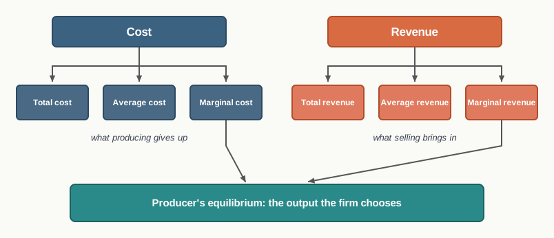
Fig. 8.0 – Cost and revenue in a firm’s output decision.
8.1 Basic Concepts of Cost
A firm cannot produce anything without using factor services, and every unit of a factor used in one line of production is a unit denied to another. The value of what is given up in this way is the cost of production of a commodity, and it is the first of the two things a producer must know before deciding how much to make.
The word ‘cost’, however, is used in more than one sense. An accountant records what the firm has actually paid out; an economist counts in addition what the firm has forgone by using resources of its own; society counts the burden that production places on people who are not part of the firm at all. Each sense answers a different question, and an exact answer in economics depends on keeping them apart.
8.1.1 Money Cost and Explicit Cost
In ordinary use, the cost of production means money cost — the money expenses a firm has to incur in purchasing or hiring the factor services it needs. These are the payments the firm actually makes to outsiders:
- wages and salaries paid to labour
- payments for raw materials, power and fuel
- rent of hired land, factory building or godown
- interest on borrowed capital
- expenses on transport, insurance, licence fees and indirect taxes
Because every one of these payments passes through the firm’s books of account, money cost is also called ‘accounting cost’ or ‘business cost’. Looked at as the price paid to the owners of factor services bought or hired from outside, the same payments are called explicit cost.
Money cost takes the cost of production in a restricted sense. A producer very often supplies some of the factor services himself, and for these no money changes hands. Nothing is entered in the account books, and to that extent the accountant’s figure understates what production has really cost.
8.1.2 Implicit Cost and Normal Profit
An entrepreneur may work in his own firm, run it from his own building and finance it with his own capital. He makes no payment to himself for any of this, but the services are not free. By using them in his own unit he gives up the salary, rent and interest he could have earned by selling those very services to some other producer, and that forgone earning is a genuine cost of his own production.
Since no payment is made, such a cost has to be imputed, that is, estimated from what the self-owned resource could have earned in its best alternative use. A cost arrived at in this way is called implicit cost.
The entrepreneur also bears the risk of production, and he will bear it only if he expects a certain minimum return. That minimum return is called normal profit. It is the supply price of entrepreneurial services in the same way that the wage is the supply price of labour, and since production stops in the long run without it, the economist treats it as a part of cost rather than as a surplus over cost.
Explicit and implicit costs differ in what is paid, in what is recorded and in how each is arrived at. The main points of difference are set out below.
8.1.3 Economic Cost
The economist takes the cost of production in the wider sense of economic cost, which counts every resource used up in production, whether it was bought from outside or already owned. It has three components:
- Explicit cost — the money payments made for the factor services bought or hired from others.
- Implicit cost — the imputed earnings of the factor services the firm owns and uses itself.
- Normal profit — the minimum return that keeps the entrepreneur in this line of production.
The two ways of measuring the cost of the same output can now be set side by side. Accounting cost stops at what the firm has paid out; economic cost adds to it what the firm has forgone.
\[\text{Money cost} = \text{Accounting cost} = \text{Explicit cost}\]
\[\text{Economic cost} = \text{Explicit cost} + \text{Implicit cost (including normal profit)}\]
Here explicit cost is the payment actually made for hired factor services and implicit cost is the imputed earning of the firm’s own factor services, both measured in rupees for a given period of production. The result is read as the full cost of using all the resources engaged in production, whoever owns them, so economic cost can never be smaller than accounting cost and is usually larger. A firm that just covers its economic cost is therefore not earning nothing — it is earning exactly the normal profit that keeps it in business.
8.1.4 Real Cost
Money cost and economic cost both measure the cost of production in rupees. Real cost looks behind the money at what production demands of people: the toil and fatigue of the worker, the abstinence of the saver who postpones consumption so that capital can be built up, and the anxiety of the entrepreneur who carries the risk.
The concept explains why factors of production have to be paid at all, but it has little practical use. Effort and sacrifice are felt differently by different people and cannot be measured, so no producer can arrive at a figure for real cost or take a decision on the strength of it.
8.2 Opportunity Cost
Every resource a firm uses is scarce, and scarcity means that a resource put to one use is withdrawn from another. A plot of land under wheat is not under mustard; an hour of a mechanic’s time spent on one repair is not spent on the next customer. Choosing, therefore, always costs something, and what it costs is whatever had to be surrendered.
This is the sense in which cost is most basic to economics. Before a payment is made or an account is written up, a choice has already been made about where a scarce resource shall go, and the value of the use it has been kept out of is the cost of the use it has been put to.
8.2.1 Meaning of Opportunity Cost
Suppose a plot of land, with a given amount of labour and capital, can raise 200 quintals of wheat, or 150 quintals of mustard, or 90 quintals of fodder in a season. Only one of these can be grown. If the farmer grows wheat, he surrenders the mustard crop and the fodder crop together, but the sacrifice that measures his cost is the best of the two he has given up, namely the 150 quintals of mustard. The choice is set out in Fig. 8.1.
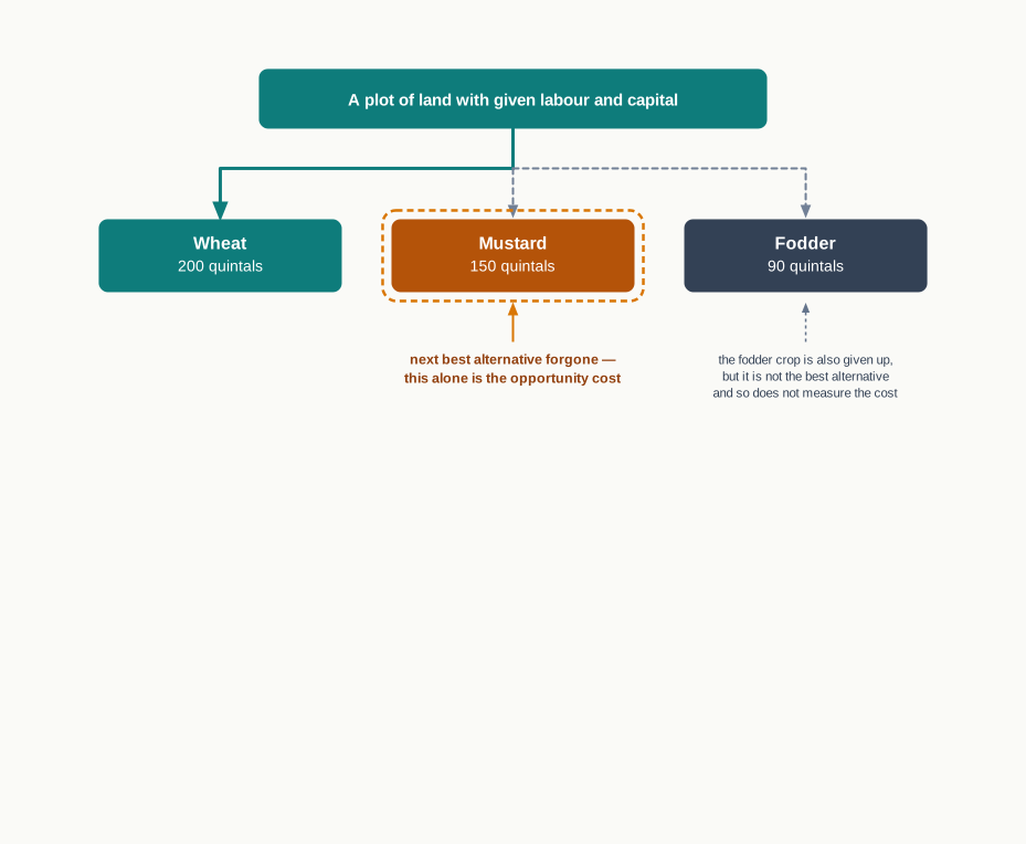
Fig. 8.1 – Opportunity cost of a plot of land.
Expressed in money, opportunity cost turns out to be the same thing as the economic cost of Section 8.1. A factor bought or hired from outside is priced at what it could earn elsewhere, and that price is the explicit cost. A factor the firm already owns earns nothing recorded, and the rent, interest or salary it forgoes is the implicit cost. Add the two and the whole of what the firm’s resources could have earned in their next best uses has been counted, which is exactly the economic cost of the output.
The idea reaches well beyond a single firm, and ISC has asked for its applications more than once. Three are worth stating.
- Pricing of factor services — a factor must be paid at least what it can earn in its next best employment, or it will move away to that employment. Opportunity cost therefore sets a floor under wages, rent and interest.
- Choice of what to produce — a producer weighing two products compares the return from one against the return surrendered on the other, so the alternative forgone decides the composition of output.
- Allocation of public funds — money the government commits to one head is money no longer available for another, so every budget allocation is judged against the head that has been passed over.
8.2.2 Opportunity Cost and Accounting Cost
Accounting cost and opportunity cost look at the same act of production from opposite ends. The accountant records what has left the firm: a bill met, a wage paid, a rent remitted. The economist asks what the firm let go of: the earning the resources would have brought in their best alternative use, whether or not any payment was made for them.
The difference matters most where a firm uses what it already owns. A trader who runs his business from his own godown enters no rent in his accounts, so his accounting cost is untouched by the building; but he has given up the rent the godown would have fetched, and his opportunity cost carries that amount. Accounting cost, in short, is confined to explicit cost, while opportunity cost takes in implicit cost as well.
The two also serve different purposes. Accounts are drawn up to record what has happened, to satisfy the tax authorities and to be audited; opportunity cost is worked out to decide what should be done next with resources that could be used in more than one way. The main points of difference are set out below.
Because a producer is choosing among uses rather than merely recording payments, price and output decisions are taken on opportunity cost. That is the reason the economist’s cost of production is economic cost, and the reason the cost schedules built up in the sections that follow are meant to be read as schedules of what production has caused the firm to give up.
8.3 Total Costs in the Short Run
The theory of cost asks a single question: how does the cost of a firm behave as its output changes? The answer depends on how far the firm is free to alter the quantities of the factors it uses, and that freedom depends on the length of the period under consideration.
The short run is the period in which at least one factor cannot be altered, so output can be raised only by working the existing plant harder. The long run is the period long enough for every factor, including the plant itself, to be varied. This section takes the short run and follows the total costs of a firm as output rises.
8.3.1 Fixed Factors and Variable Factors
In the short run the factors a firm uses fall into two groups. Fixed factors — the factory building, the machinery installed in it, the permanent staff — cannot be increased or decreased whatever the level of output. Variable factors — raw materials, power, casual labour — can be had in any quantity the firm wants, and are used in larger amounts as more is produced.
The distinction is one of period, not of the factor itself. A weaving shed is a fixed factor over the coming season and a variable one over five years, because in five years sheds can be built or sold. The main points of difference are set out below.
Corresponding to these two groups of factors, the cost of a firm in the short run divides into fixed cost and variable cost, and the two together make up total cost.
8.3.2 Total Fixed Cost
Total fixed cost is the cost a firm incurs on its fixed factors. It is settled before production begins and does not move with output, so the firm carries the same burden on this account whether it turns out one unit, a hundred units or none at all. The commonest items are:
- rent of the factory building and land
- interest on capital borrowed for plant and machinery
- depreciation of machinery and expenses on its upkeep
- salaries of permanent staff and managers
- property tax, licence fee and insurance premium
Because it must be met even when the plant lies idle, fixed cost is also called ‘unavoidable cost’, ‘supplementary cost’ or ‘overhead cost’. A shopkeeper pays the rent of his shop for a month in which a strike kept it shut, and a mill pays interest on its loan in a month in which no cloth left the gate.
The behaviour of the three total costs of a small firm is set out in Table 8.1, which will be used through the rest of this section.
Column 2 of Table 8.1 stands unchanged at ₹60 from zero output to six units. Plotted against output, it gives a horizontal straight line, as shown in Fig. 8.2.
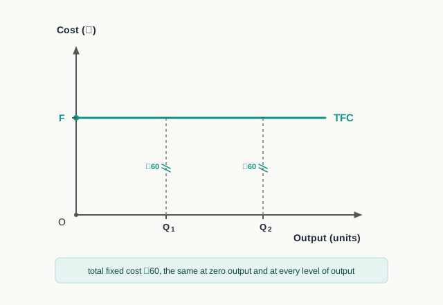
Fig. 8.2 – Total fixed cost curve.
The curve begins on the Y-axis and not at the origin, and that starting point carries the whole meaning of fixed cost: at zero output the firm is already ₹60 out of pocket.
8.3.3 Total Variable Cost
Total variable cost is the cost a firm incurs on its variable factors. Since these factors are employed in proportion to what is being made, this cost is zero when output is zero and rises as output rises. Its usual items are:
- expenditure on raw materials
- wages paid to casual and temporary workers
- power, fuel and water used in production
- transport of materials and finished goods
- excise and other duties that depend on the quantity produced
Variable cost is not incurred if nothing is produced, so it is also called ‘avoidable cost’, ‘prime cost’ or ‘direct cost’.
Column 3 of Table 8.1 shows that total variable cost does not rise evenly. The successive additions are ₹40 and ₹26 for the first two units, and then ₹30, ₹36, ₹53 and ₹61 for the next four. Variable cost thus rises at a decreasing rate up to the second unit and at an increasing rate beyond it, which gives the curve in Fig. 8.3 its inverted S shape.
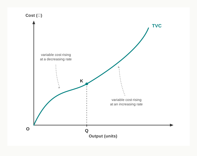
Fig. 8.3 – Total variable cost curve.
The reason lies in the law of variable proportions, since cost and productivity are two sides of one coin. While the fixed plant is being filled up, extra doses of the variable factor yield increasing returns and each additional unit of output is obtained more cheaply. Once the plant is fully used, the variable factor crowds upon it, returns diminish and each additional unit costs more than the one before.
Fixed and variable cost may now be placed side by side, since almost every question on short-run cost turns on the difference between them.
8.3.4 Total Cost and the Total Cost Curves
Total cost is the whole obligation a firm incurs in producing a given quantity of output, on fixed and variable factors together. It is therefore obtained by adding the two totals already described.
\[\text{TC} = \text{TFC} + \text{TVC}\]
Here TC is total cost, TFC total fixed cost and TVC total variable cost, all three measured in rupees for the same output and the same period. The result is read as the entire cost of that output; and since TFC is a constant, every change in TC from one level of output to the next is due to the change in TVC alone.
Column 4 of Table 8.1 bears this out. Total cost is ₹60 at zero output, where it equals total fixed cost, and thereafter it rises by exactly the amounts by which variable cost rises — ₹40, ₹26, ₹30, ₹36, ₹53 and ₹61. Fig. 8.4 places all three curves in one diagram.
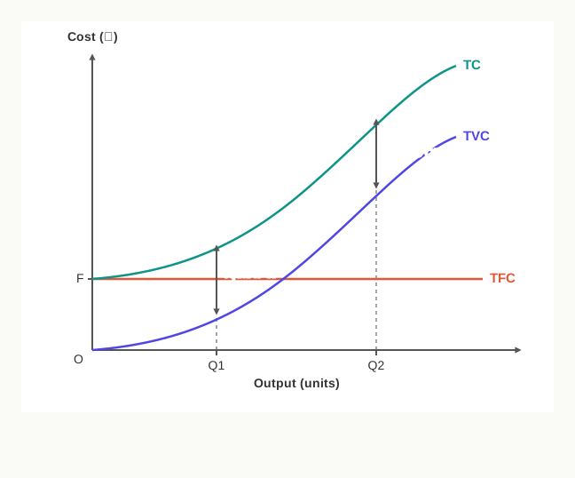
Fig. 8.4 – Total cost and its components.
Three features of the diagram should be fixed in mind. The TC curve starts from F and not from the origin, because at zero output total cost equals total fixed cost. The TC curve is obtained by adding the TFC line vertically to the TVC curve, so it has the same shape as TVC and rises at a decreasing rate first and at an increasing rate afterwards. And the vertical distance between TC and TVC never narrows, since it measures a fixed cost that does not change with output.
Because the three totals are tied together by one equation, any two of them give the third. The commonest exercise is to be handed a total cost schedule and asked to separate it, as in Table 8.2 and SE 8.1.
8.4 Per Unit Costs in the Short Run
The total costs of Section 8.3 answer one question: what does a given output cost the firm altogether? A producer, however, has to answer two further questions before he can decide anything. What does a unit of the commodity cost him on an average, and what does one more unit add to his cost?
The first question is answered by the average costs and the second by marginal cost. These per unit costs, and not the totals, are the figures a firm compares with the price it can get, which is why the theory of price is built on them. All four are worked out in Table 8.4 for the same firm whose totals were set out in Table 8.1.
8.4.1 Average Fixed Cost
Average fixed cost answers the question of what share of the firm’s overheads each unit of output has to carry. It is found by spreading the whole of the fixed cost over the units produced.
\[\text{AFC} = \dfrac{\text{TFC}}{Q}\]
Here TFC is total fixed cost in rupees and \(Q\) is the number of units produced in the period. The result is read as the rupees of fixed cost borne by one unit of output.
Column 5 of Table 8.4 falls steadily, from ₹60 at one unit to ₹10 at six units. The reason is plain from the formula: the numerator is a constant ₹60 while the denominator grows, so the same overhead is divided among more and more units. This is the whole meaning of ‘spreading the overhead’, and it is why a plant that is worked near its capacity carries a lighter fixed burden on each unit than one that stands half idle.
Average fixed cost falls throughout, but it can never reach zero, because a positive fixed cost divided by any number of units still leaves something to be borne. Its curve therefore comes closer and closer to the X-axis without ever touching it, and at very small outputs it rises very steeply without ever touching the Y-axis. Such a curve is called a rectangular hyperbola: at every point on it, average fixed cost multiplied by output gives the same figure, namely total fixed cost. Fig. 8.5 shows its shape.
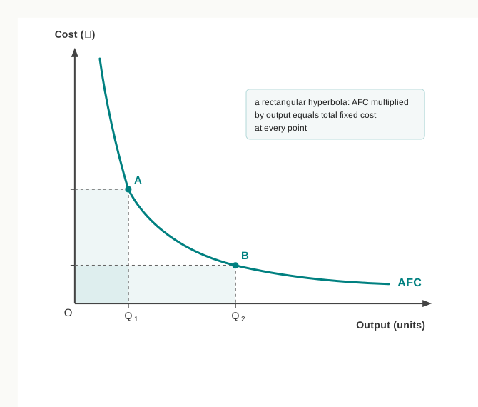
Fig. 8.5 – Average fixed cost curve.
8.4.2 Average Variable Cost
Average variable cost is what each unit costs the firm in materials, power and hired labour, leaving the overheads out.
\[\text{AVC} = \dfrac{\text{TVC}}{Q}\]
Here TVC is total variable cost in rupees for the period and \(Q\) is the number of units produced. The result is read as the rupees of variable cost borne by one unit of output.
Column 6 of Table 8.4 behaves quite differently from average fixed cost. It falls from ₹40 to ₹32 as output rises to three units, and then turns and rises to ₹41 at six units. Plotted against output, a series of this kind gives a U-shaped curve, and the output at which it is lowest — three units for this firm — is called the optimum capacity level of output, since it is there that the variable factors are being used to best advantage.
The U-shape follows directly from the law of variable proportions. At small outputs the fixed plant is under-used and there is too little of the variable factor to work it properly; as more of the variable factor is applied, the plant is used more fully, specialisation becomes possible, returns to the variable factor increase and the cost of each unit falls. Beyond the optimum the plant has been used to the full, the variable factor begins to crowd upon it, returns diminish, and each unit costs more than the one before.
8.4.3 Average Total Cost
Average total cost, or simply average cost, is what a unit of output costs on all counts together, fixed and variable.
\[\text{ATC} = \dfrac{\text{TC}}{Q}\]
Here TC is total cost in rupees and \(Q\) is output in units, so the result is read as the rupees of total cost borne by one unit. Since total cost is itself the sum of the two other totals, the same figure can be reached a second way.
\[\text{ATC} = \dfrac{\text{TFC} + \text{TVC}}{Q} = \dfrac{\text{TFC}}{Q} + \dfrac{\text{TVC}}{Q} = \text{AFC} + \text{AVC}\]
Average total cost is therefore the vertical sum of average fixed cost and average variable cost at each level of output. In Table 8.4, at four units, ₹15 of average fixed cost and ₹33 of average variable cost together give the ₹48 shown in column 7.
Average total cost is U-shaped for the same reason as average variable cost, and its lowest point — ₹48 at four units for this firm — is called the optimum point of production, the output at which the commodity is produced most cheaply per unit.
Two features of the relation between the two U-shaped curves must be noticed, and both can be read off Table 8.4. First, average total cost lies above average variable cost at every output, and the gap between them is exactly average fixed cost. Since average fixed cost falls as output rises, the gap narrows as we move to the right; but as it never becomes zero, the two curves come closer and closer without ever meeting. Second, the minimum of average total cost comes at a larger output than the minimum of average variable cost — four units against three. The reason is that after three units, average variable cost has begun to rise, but average fixed cost is still falling fast enough to more than offset the rise, so average total cost goes on falling for a while yet. Fig. 8.6 brings the three average curves together.
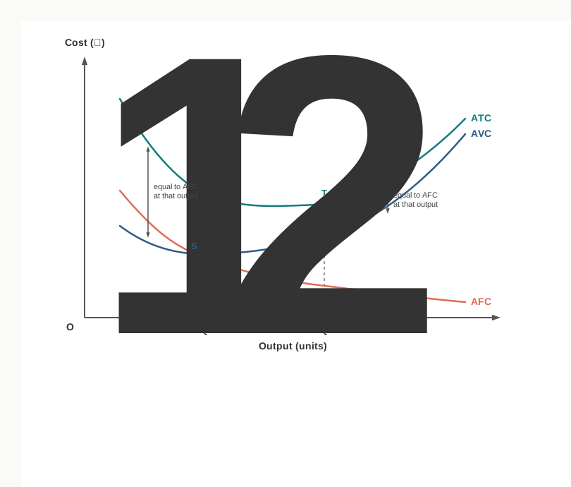
Fig. 8.6 – Average cost curves.
8.4.4 Marginal Cost
Marginal cost answers the producer’s sharpest question: what does one more unit add to my cost? It is not an average of anything but a difference between two totals.
\[\text{MC}_n = \text{TC}_n - \text{TC}_{n-1}\]
Here \(\text{TC}_n\) is the total cost of producing \(n\) units and \(\text{TC}_{n-1}\) the total cost of producing one unit less, both in rupees. The result is read as the rupees added to total cost by the \(n\)th unit of output. Where output changes by more than one unit at a time, the same idea is written as a ratio.
\[\text{MC} = \dfrac{\Delta \text{TC}}{\Delta Q}\]
Here \(\Delta \text{TC}\) is the change in total cost in rupees and \(\Delta Q\) the change in output in units, so marginal cost is the addition to total cost per unit of additional output, and diagrammatically it is the slope of the total cost curve at that output.
Column 8 of Table 8.4 is obtained by taking these differences down the total cost column: ₹100 − ₹60 = ₹40 for the first unit, ₹126 − ₹100 = ₹26 for the second, and so on to ₹61 for the sixth.
Three points about marginal cost deserve attention.
- Marginal cost is independent of fixed cost — total fixed cost does not change when one more unit is produced, so the whole of the addition to total cost comes from the addition to variable cost. Marginal cost can therefore be found from the variable cost column just as well as from the total cost column, and the two give identical answers.
- Total variable cost is the sum of the marginal costs — since each unit adds its own marginal cost to the total, adding up the marginal costs of all the units produced gives total variable cost. In Table 8.4 the six marginal costs add up to ₹246, which is precisely the total variable cost of six units.
- Marginal cost is U-shaped — it falls while the variable factor is yielding increasing returns, reaches a minimum, and rises once diminishing returns set in. In Table 8.4 it falls to ₹26 at the second unit and rises steadily thereafter.
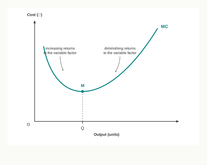
Fig. 8.7 – Marginal cost curve.
The marginal cost curve reaches its lowest point at a smaller output than either of the U-shaped average curves, as Table 8.4 shows — marginal cost is least at the second unit, average variable cost at the third and average total cost at the fourth. Why the three minima fall in this order, and how the marginal curve pulls the average curves down and then pushes them up, is taken up in Section 8.5.
8.5 Relationship Between Average Cost and Marginal Cost
Average cost and marginal cost are drawn from the same total cost, one by dividing it and the other by taking differences down it. Two magnitudes obtained from a common source cannot move independently, and the way they move together is one of the most closely questioned points in the theory of cost.
The relationship is also the bridge to the rest of the chapter. A producer decides how much to produce by comparing marginal cost with marginal revenue, and judges whether that output is worth producing at all by comparing average cost with price, so the two must first be understood in relation to each other.
8.5.1 The Three Cases of the Relationship
The two costs answer different questions and are arrived at differently. The main points of difference are set out below.
The link between them is a matter of arithmetic before it is a matter of economics. Whenever a fresh item is added to a group, the average of the group is pulled towards that item. A batsman with an average of 40 who scores 20 in his next innings sees his average fall; if he scores 60 it rises; if he scores exactly 40 it stays where it was. Marginal cost is the fresh item added to the firm’s cost record, and average cost is the average of the group. Three cases follow.
- When marginal cost is less than average cost, average cost falls — the unit just produced has cost less than the average of all the earlier units, so it pulls the average down. In the diagram the MC curve lies below the AC curve and the AC curve slopes downward.
- When marginal cost is greater than average cost, average cost rises — the unit just produced has cost more than the average, so it pulls the average up. The MC curve lies above the AC curve and the AC curve slopes upward.
- When marginal cost is equal to average cost, average cost is constant — the unit just produced has cost exactly what the earlier units cost on an average, so the average is neither pulled down nor pushed up. This happens at the lowest point of the AC curve.
The schedule of the firm used in Section 8.4 shows all three cases at work. Table 8.5 sets the two columns side by side.
The arithmetic can be followed unit by unit. At three units the firm’s average total cost is ₹52; the fourth unit costs only ₹36, so the average of the four is pulled down to ₹48. The fifth unit costs ₹53, which is more than the ₹48 the earlier units averaged, and the average is pushed up to ₹49. Between the two lies the output at which the pull and the push balance, and there average cost is at its minimum.
Exactly the same holds between marginal cost and average variable cost. Marginal cost lies below average variable cost up to three units, where average variable cost falls to its lowest figure of ₹32, and above it thereafter, when average variable cost turns upward. Marginal cost is drawn from total cost and from total variable cost alike, so it bears the same relation to both average curves, as Fig. 8.8 shows.
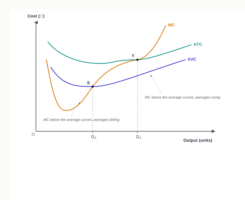
Fig. 8.8 – Marginal cost cutting average cost curves at their minima.
One caution must be entered. The relationship is about the direction in which average cost moves and the magnitude of marginal cost — whether marginal cost is above or below the average — and about nothing else. It tells us nothing about the direction in which marginal cost itself is moving. Between the minimum of the marginal cost curve and the minimum of the average cost curve, marginal cost is rising while average cost is still falling, because each additional unit costs more than the one before and yet less than the running average. Fig. 8.9 marks that range off.
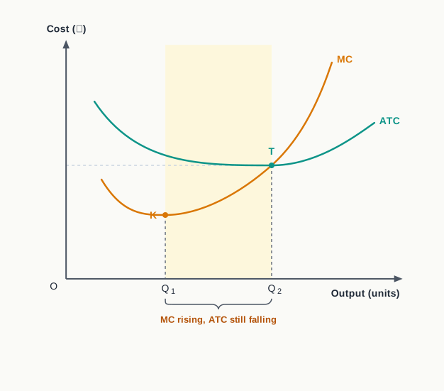
Fig. 8.9 – A rising marginal cost with a falling average cost.
8.5.2 Why MC Cuts AC at Its Minimum Point
The three cases together settle both the point at which the marginal cost curve meets the average cost curve and the direction from which it comes.
To the left of the lowest point of the average cost curve, average cost is falling, and by the first case marginal cost must be lying below it. To the right of that point average cost is rising, and by the second case marginal cost must be lying above it. A curve that is below another on one side of a point and above it on the other must pass through that point, and must pass through it going upward — that is, it must cut the average cost curve from below.
The point of intersection can only be the minimum of the average cost curve. It is the one output at which average cost has stopped falling but has not yet begun to rise, so by the third case it is the one output at which marginal cost equals average cost. This is why the intersection is often used to identify the optimum point of production: the output at which the commodity is produced at the least cost per unit is the output at which marginal cost equals average cost.
8.6 Cost in the Long Run
Everything in Sections 8.3 to 8.5 rested on one restriction: the plant was given. A firm working a fixed shed with fixed machinery can raise output only by pressing more variable factors upon them, and it is that pressure which finally forces cost per unit up.
Given time, the restriction disappears. Over a long enough period a firm can install another machine, extend the shed or build a new factory altogether, and it can equally let a plant go. In the long run, therefore, every factor is variable, and the firm is free to produce each level of output with the size of plant best suited to it.
Two consequences follow at once. There is no fixed cost in the long run, so there is nothing corresponding to TFC or AFC, and only three curves remain — long-run total cost, long-run average cost and long-run marginal cost. And long-run cost is always a least cost: for every output, the firm is assumed to have chosen the plant that produces it as cheaply as possible.
8.6.1 Long-Run Total Cost
Long-run total cost is the least cost of producing each level of output when all the factors of production, including the plant, can be varied. For any output the firm looks over every size of plant open to it, and the lowest total cost it can find is the long-run total cost of that output.
The curve is drawn in Fig. 8.10. It starts from the origin, because with nothing fixed a firm that produces nothing incurs no cost at all — a plain contrast with the short-run total cost curve, which starts on the Y-axis at the level of fixed cost. It rises throughout, since more output always needs more resources, and like the short-run curve it has an inverse S shape: cost rises at a decreasing rate at first and at an increasing rate later. The reason for the change of curvature, however, is a different one, and is taken up in Section 8.6.4.
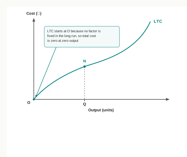
Fig. 8.10 – Long-run total cost curve.
8.6.2 Long-Run Average Cost
Long-run average cost is long-run total cost divided by output. Since the long-run total is a least cost, the average is the lowest per unit cost at which each output can be produced once the firm is free to choose its plant.
Each possible plant has a short-run average cost curve of its own, and the firm cannot escape that curve once the plant is built. In the long run it is not tied to any one of them: for a small output it selects the small plant, for a larger output the larger plant. The long-run average cost curve is therefore drawn as the boundary that lies under all the short-run curves, touching each of them at the one output for which that plant is the cheapest. Because it wraps round the family of short-run curves in this way, it is called an envelope curve, and because a firm consults it when deciding what plant to build, it is also called the planning curve. Fig. 8.11 shows the construction; the formal derivation is not required.
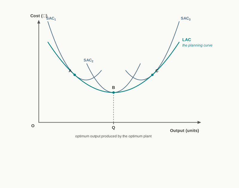
Fig. 8.11 – Long-run average cost curve as an envelope.
The long-run average cost curve is U-shaped, but its U is flatter than that of any short-run curve, and its lowest point B marks the optimum plant producing the optimum output — the cheapest way of making the commodity that is open to the firm at all.
8.6.3 Long-Run Marginal Cost
Long-run marginal cost is the addition made to long-run total cost when one more unit of output is produced, with every input, including the plant, adjusted to suit that output.
Its relationship with long-run average cost is exactly the relationship established in Section 8.5, for the arithmetic that produced it does not change with the length of the period. Long-run marginal cost lies below long-run average cost while the latter is falling, lies above it while the latter is rising, and equals it at the lowest point of the LAC curve, which it therefore cuts from below. The LMC curve is U-shaped like the LAC curve and, like it, flatter than its short-run counterpart. Fig. 8.12 sets the two together.
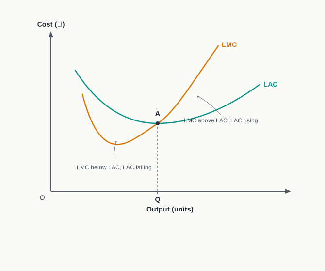
Fig. 8.12 – Long-run average and marginal cost.
8.6.4 Economies and Diseconomies of Scale
Why should long-run average cost fall at all, and why should it turn upward again? The answer cannot be the law of variable proportions, since in the long run no factor is held fixed and there are no proportions to disturb. It lies instead in the advantages and disadvantages that come with the scale of production itself.
As a firm expands its scale, it gains certain advantages — larger and more specialised machinery becomes worth installing, work can be divided more finely, materials and credit can be obtained on better terms — and its average cost falls. These are the economies of scale, also described as increasing returns to scale. Pushed beyond a point, expansion brings the opposite: the organisation grows too large to be supervised closely, decisions are delayed and coordination suffers, so average cost rises. These are the diseconomies of scale, or decreasing returns to scale. The falling stretch of the LAC curve is the work of the first and the rising stretch the work of the second.
Economies and diseconomies are of two kinds according to where they come from. Internal economies arise within the firm, from the growth of its own scale.
The main internal economies may be stated briefly.
- Technical economies — a larger output makes it worth installing bigger and more specialised machinery, which produces each unit more cheaply.
- Managerial economies — a large firm can employ specialists for purchase, production and sales, and their salaries are spread over a much larger output.
- Marketing economies — bulk purchase of materials and bulk transport of the finished product are obtained on better terms.
- Financial economies — a large firm borrows more easily and at lower rates of interest than a small one.
Where expansion is carried too far, the same sources turn into internal diseconomies: management is stretched beyond the reach of effective supervision, communication within the firm slows and mistakes multiply, and cost per unit rises.
External economies, in contrast, do not depend on the size of any one firm. They arise when the industry as a whole grows, and they are shared by every firm in it, large or small.
When a centre grows beyond what its roads, power supply and housing can carry, the advantage turns the other way. Rents and wages are bid up, transport is congested and inputs grow dearer, and every firm in the industry finds its costs higher. These are external diseconomies. Internal economies and diseconomies decide the shape of a firm’s LAC curve; external economies and diseconomies move the whole curve down or up.
8.7 Concepts of Revenue
Cost tells a producer what an output has taken out of him. Revenue tells him what it has brought in. Revenue means the receipts of a firm from the sale of its product in a given period, and since a firm produces in order to sell, no decision about output can be taken without it.
Revenue must not be confused with profit. Revenue is the whole of the sale proceeds; profit is what is left of those proceeds after the cost of production has been met. Just as cost was studied as a total, as an average and at the margin, revenue is studied under three heads — total revenue, average revenue and marginal revenue — set out in Fig. 8.13.
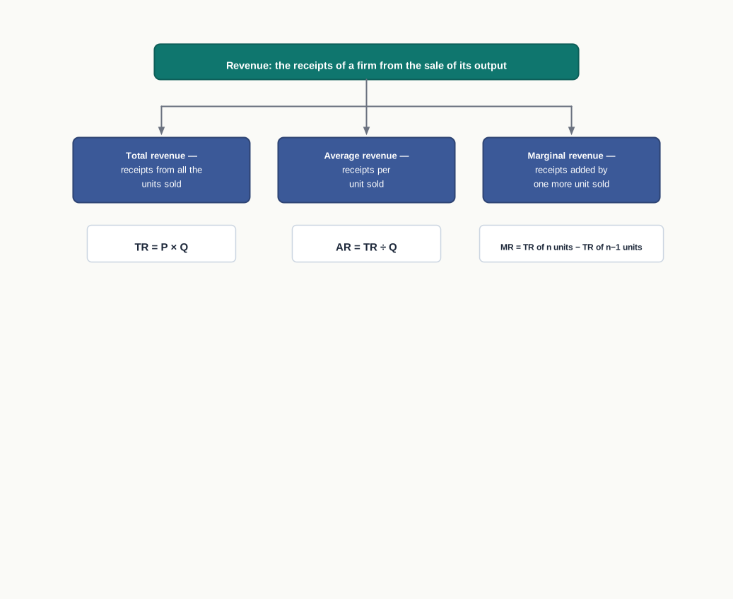
Fig. 8.13 – The three concepts of revenue.
8.7.1 Total Revenue
Total revenue is the whole amount a firm receives by selling a given quantity of its product. It depends on two things together — how much is sold and at what price — so it is arrived at by multiplying the one by the other.
\[\text{TR} = P \times Q\]
Here \(P\) is the price per unit in rupees and \(Q\) is the number of units sold in the period. The result is read as the rupees the firm takes in from that sale: a firm selling 12 units at ₹25 each has a total revenue of ₹300.
Total revenue looked at from the firm’s side is the same sum of money as the expenditure of the buyers looked at from theirs; the two are two sides of one transaction. How total revenue behaves as the firm sells more depends on whether the price stays put or has to be reduced, and that is a question of the market the firm sells in, taken up in Sections 8.8 and 8.9.
8.7.2 Average Revenue
Average revenue is the revenue earned per unit of the product sold. It is obtained by spreading total revenue over the units sold.
\[\text{AR} = \dfrac{\text{TR}}{Q} = \dfrac{P \times Q}{Q} = P\]
Here TR is total revenue in rupees, \(Q\) the number of units sold and \(P\) the price per unit. The working shows something important: when all the units are sold at the same price, as is normally the case, average revenue works out to the price itself. The result is read as the rupees the firm gets for one unit.
Because average revenue is the price, the average revenue curve of a firm is the demand curve for its product: it shows the price at which each quantity can be sold. This is the concept of revenue that ISC questions describe as ‘price’.
8.7.3 Marginal Revenue
Marginal revenue is the addition made to total revenue when one more unit of the product is sold. Like marginal cost, it is a difference between two totals and not an average of anything.
\[\text{MR}_n = \text{TR}_n - \text{TR}_{n-1}\]
Here \(\text{TR}_n\) is the total revenue from selling \(n\) units and \(\text{TR}_{n-1}\) that from selling one unit less, both in rupees. The result is read as the rupees added to total revenue by the \(n\)th unit. Where sales change by more than one unit at a time the same idea is written as a ratio.
\[\text{MR} = \dfrac{\Delta \text{TR}}{\Delta Q}\]
Here \(\Delta \text{TR}\) is the change in total revenue in rupees and \(\Delta Q\) the change in the quantity sold, so marginal revenue is the addition to total revenue per unit of additional sale, and diagrammatically it is the slope of the total revenue curve.
Since every unit sold adds its own marginal revenue to the total, the marginal revenues of all the units sold add up to total revenue.
\[\text{TR} = \Sigma \text{MR}\]
Here \(\Sigma \text{MR}\) is the sum of the marginal revenues of every unit sold up to that quantity, in rupees, and the equation is read as saying that total revenue at any level of sales can be built up from the marginal revenue column just as it can be read off the total revenue column.
The three concepts are worked out in Table 8.6 for a firm that has to lower its price a little to sell each additional unit.
Two things may be checked in the table. Average revenue in column 2 is the price at which each quantity is sold, and total revenue in column 3 is that price multiplied by the quantity. The marginal revenues in column 4 add up to ₹80 for five units — 24 + 20 + 16 + 12 + 8 — which is exactly the total revenue shown against five units.
The three concepts are compared below on the points that questions usually turn on.
8.8 Revenue Under Perfect Competition
Unlike cost, revenue has no single theory that fits every firm. The three concepts of Section 8.7 are defined in the same way for all firms, but how they behave as output rises depends entirely on the terms on which a firm can sell — on whether it can dispose of more units at the going price, or must shade the price down to find buyers for them.
That, in turn, depends on the market. Two situations have to be distinguished: a perfectly competitive market, taken up here, and an imperfectly competitive market, taken up in Section 8.9.
Under perfect competition a very large number of firms sell a homogeneous product, and the output of any one of them is too small a part of the total to affect the price. The price is settled for the market as a whole, and the individual firm takes it as given: it can sell as much or as little as it likes at that price, and nothing at all above it. The firm is, in the familiar phrase, a price-taker, and the market forms in which this holds are examined fully in a later chapter.
8.8.1 Behaviour of Average and Marginal Revenue
Two conclusions follow directly from the firm’s position as a price-taker, and Table 8.7 sets them out for a firm selling at a ruling price of ₹15.
First, average revenue is constant and equal to the price. Every unit is sold at ₹15, so the receipts per unit are ₹15 at every level of sales, and column 4 does not move.
Second, marginal revenue is equal to average revenue. An extra unit is sold at the ruling price without any reduction on the units already being sold, so it adds exactly ₹15 to total revenue, which is precisely the price. Column 5 therefore repeats column 4. Under perfect competition, in short:
\[\text{AR} = \text{MR} = P\]
Here \(P\) is the ruling market price in rupees per unit, and AR and MR are average and marginal revenue in the same units. The equality is read as saying that for a price-taking firm the price, the receipts per unit and the addition made by one more unit are three names for one figure.
Drawn against output, both are the same horizontal straight line at the height of the ruling price, as in Fig. 8.14. Since the line shows the quantities the firm can sell at that price, it is also the demand curve facing the firm, and it is perfectly elastic: the firm can sell any amount at ₹15 and nothing above it.
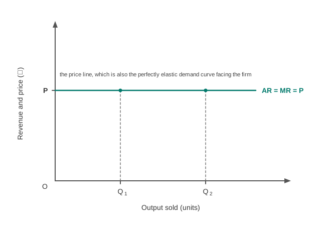
Fig. 8.14 – Average and marginal revenue under perfect competition.
8.8.2 Behaviour of Total Revenue
Total revenue, unlike the other two, does change as the firm sells more. Column 3 of Table 8.7 rises from ₹15 to ₹75, and it rises by the same ₹15 with every additional unit, since each unit fetches the unchanged price.
A magnitude that increases by a constant amount for every unit added gives a straight line when it is plotted, and one that begins at the origin, because a firm that sells nothing earns nothing. Total revenue therefore varies in direct proportion to output: sales of four units bring in exactly twice what sales of two units bring in. Fig. 8.15 shows the curve.
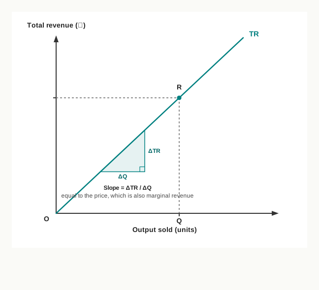
Fig. 8.15 – Total revenue under perfect competition.
The slope of the total revenue line is worth a moment. Marginal revenue is the addition to total revenue per unit of additional sale, which is exactly what the slope of the total revenue curve measures. Under perfect competition marginal revenue is constant, so the slope is constant, and the curve is a straight line. This is the same reasoning that will be used in Section 8.9, where a falling marginal revenue produces a total revenue curve that bends.
8.9 Revenue Under Imperfect Competition
A firm selling under monopoly, monopolistic competition or oligopoly is not lost in a crowd of sellers. Its output is a substantial part of what reaches the market, or its product is marked off from its rivals’ by brand, quality or location, and buyers will take more of it only at a lower price. Such a firm faces a downward sloping demand curve, and it is a price-maker to the extent that it can choose a point on that curve.
The consequence is decisive for revenue. To sell an extra unit the firm must reduce the price, and — since the units are identical to the buyer — it must reduce the price on every unit it sells, not on the extra one alone. Table 8.8 carries the schedule of Table 8.6 through to the point where this begins to hurt.
8.9.1 Behaviour of Average and Marginal Revenue
Average revenue is the price, so column 2 of Table 8.8 is the behaviour of average revenue: it falls continuously, from ₹24 to ₹10, as sales are pushed up. It falls, but it cannot fall to zero or below, because no firm sells at a price of nothing. For simplicity the fall is taken to be at a constant rate — ₹2 for each additional unit here — which gives a straight line AR curve.
Marginal revenue falls too, and much faster: ₹24, ₹20, ₹16 and so on, ₹4 at a step. Except on the first unit, where the two are equal because there are no earlier units to be affected, marginal revenue is less than average revenue at every level of sales.
The reason repays attention, and the table supplies the arithmetic. The fifth unit is sold at ₹16, so the firm gains ₹16 on it. But the four units already being sold, which would have fetched ₹18 each, now fetch only ₹16 each, a loss of ₹2 on each of the four, or ₹8 in all. The net addition to total revenue is therefore ₹16 − ₹8 = ₹8, which is the marginal revenue shown against the fifth unit.
Marginal revenue is under no obligation to stay positive. In Table 8.8 it reaches zero at the seventh unit, where the gain on the extra unit exactly cancels the loss on the earlier ones, and turns negative at the eighth. Average revenue and marginal revenue thus differ in a further respect: average revenue is always positive, while marginal revenue may be positive, zero or negative.
Fig. 8.16 draws the two curves. Both slope downward from the same point on the Y-axis, and MR falls at twice the rate of AR, so that where the AR curve is a straight line the MR curve bisects every perpendicular drawn from a point on AR to the Y-axis. This second property holds only for a straight line average revenue curve.
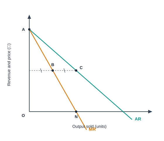
Fig. 8.16 – Average and marginal revenue under imperfect competition.
8.9.2 Behaviour of Total Revenue
Column 3 of Table 8.8 tells a story in three parts. Total revenue climbs from ₹24 to ₹84 as sales rise to six units, but it climbs by smaller and smaller amounts — ₹20, ₹16, ₹12, ₹8 and ₹4 — because each additional unit adds less than the one before. At seven units it stands still at ₹84, the extra unit having added nothing. At eight units it actually falls to ₹80.
Plotted against output, such a series gives a dome-shaped curve: rising at a diminishing rate, flattening at the top, and then turning down. Fig. 8.17 shows it.
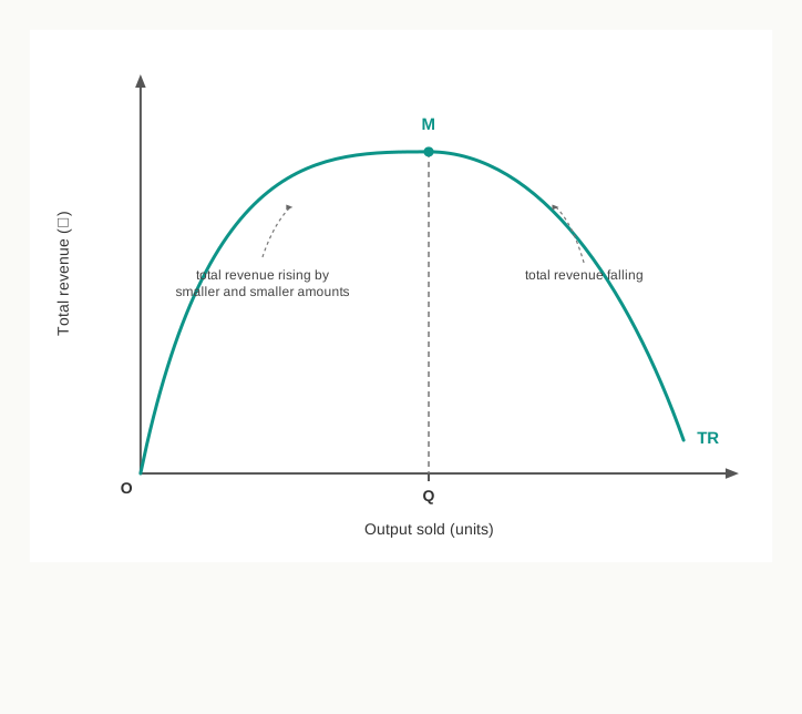
Fig. 8.17 – Total revenue under imperfect competition.
Under perfect competition the total revenue curve was a straight line through the origin, since price and marginal revenue were constant. Here the price is not constant, marginal revenue declines, and the curve bends accordingly. The shape of the total revenue curve, in other words, is settled by the behaviour of marginal revenue.
8.9.3 Relationship Between Total Revenue and Marginal Revenue
Marginal revenue is the addition made to total revenue by one more unit, so the sign of marginal revenue and the direction of total revenue must agree. Three statements cover every case, and each of them can be checked against Table 8.8 and read off Fig. 8.18.
- When marginal revenue is positive, total revenue increases with sales — up to six units in the table, marginal revenue is positive and total revenue rises, though by smaller amounts each time because marginal revenue itself is falling.
- When marginal revenue is zero, total revenue is at its maximum — at the seventh unit the extra unit adds nothing, and total revenue stays at its highest figure of ₹84. In the diagram the MR curve cuts the X-axis exactly below the top of the TR curve.
- When marginal revenue is negative, total revenue falls — the eighth unit takes ₹4 away, and total revenue drops to ₹80. Beyond this point extra sales are worse than useless to the firm’s receipts.
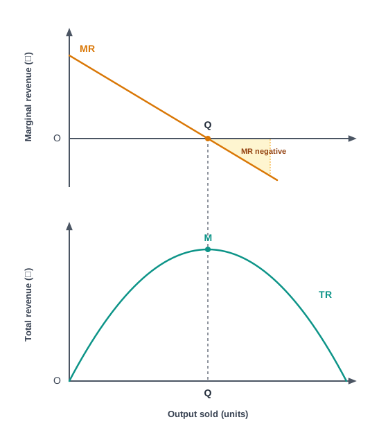
Fig. 8.18 – Total and marginal revenue compared.
The revenue position of a firm in the two kinds of market may now be set side by side, a comparison ISC has asked for more than once.
8.10 Producer’s Equilibrium
Cost and revenue have been studied separately. A producer, however, meets them together, and the whole purpose of measuring them is to settle a single question: how much should the firm produce?
8.10.1 Meaning of Producer’s Equilibrium
A firm is assumed to aim at the largest profit it can get. Profit is what is left of the receipts after the cost of production has been met.
\[\text{Profit} = \text{TR} - \text{TC}\]
Here TR is total revenue and TC is total cost, both in rupees and both for the same output and period. The result is read as the surplus the firm is left with at that output; where total cost exceeds total revenue the figure is negative and the firm is making a loss. Since economic cost already includes normal profit, a firm whose profit by this measure is zero is still earning the normal profit that keeps it in business.
The output that yields the largest profit is the output the producer settles at. At any other level he would have reason to expand or to cut back; at this one he has none, and that absence of any motive to change is what the word equilibrium means.
The same position can be reached by two routes — by comparing the totals, or by comparing the additions made at the margin. ISC requires both, each with its diagram.
8.10.2 The Total Revenue and Total Cost Approach
On this approach the producer simply looks for the output at which the excess of total revenue over total cost is greatest. Table 8.9 works it out for the firm whose cost schedule was built up in Section 8.4, now supposed to be selling in a competitive market at a price of ₹53 a unit.
Column 4 tells the whole story. At small outputs total cost exceeds total revenue and the firm loses money, mainly because the fixed cost of ₹60 is spread over too little output. The loss shrinks, turns into a profit of ₹3 at three units, and reaches ₹20 at four units and again at five. At six units profit falls to ₹12. The largest profit the firm can earn is ₹20, and the largest output at which it earns it is five units, which is therefore its equilibrium output.
Two conditions may be stated for this approach.
- Total revenue must exceed total cost, and the vertical distance between them must be the maximum — a smaller gap means a smaller profit, and no gap at all means the firm is only covering its costs.
- Beyond the equilibrium output the gap must begin to narrow — if it were still widening, the firm would gain by producing more, and the output could not be an equilibrium.
Fig. 8.19 draws the two totals for a firm selling at a fixed price.
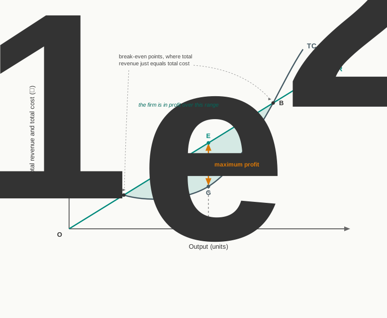
Fig. 8.19 – Producer’s equilibrium (TR and TC approach).
The tie in the profit column between four and five units is not an accident and is worth pausing over. The fifth unit adds ₹53 to revenue and ₹53 to cost, so it adds nothing to profit and takes nothing away. That is precisely the condition the second approach fastens upon.
8.10.3 The Marginal Revenue and Marginal Cost Approach
Instead of comparing the totals, the producer may ask of each additional unit whether it is worth making. The unit is worth making if it brings in more than it costs, that is, if its marginal revenue exceeds its marginal cost.
The argument then runs itself. So long as MR is greater than MC, every additional unit adds something to profit and the firm expands. If MR is less than MC, the last unit has subtracted from profit and the firm cuts back. Profit can be no larger when the two are equal, and at that point the firm stops. In Table 8.9, marginal revenue is ₹53 throughout, marginal cost is below it up to the fourth unit, equal to it at the fifth and above it at the sixth — the equilibrium is at five units, exactly as the totals showed.
Equality alone, however, is not sufficient. Marginal cost is U-shaped, so it may equal marginal revenue twice: once while it is still falling and once while it is rising. At the first of these outputs the units that follow have a marginal cost below marginal revenue, so the firm gains by producing more, and the output cannot be an equilibrium. Two conditions are therefore required.
- Marginal revenue must equal marginal cost — the last unit produced must add exactly as much to revenue as it adds to cost.
- Marginal cost must be rising at that output, so that it cuts the marginal revenue curve from below — beyond the equilibrium every further unit must cost more than it fetches.
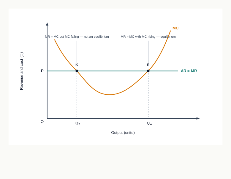
Fig. 8.20 – Producer’s equilibrium (MR and MC approach) under perfect competition.
The two conditions hold whatever the market form; only the shape of the marginal revenue curve changes. Under perfect competition MR is the horizontal price line of Fig. 8.20. Under imperfect competition MR slopes downward and lies below AR, as Section 8.9 showed, and the rising marginal cost curve cuts it from below at the equilibrium output, the price being read off the average revenue curve above that output. Fig. 8.21 shows this case.
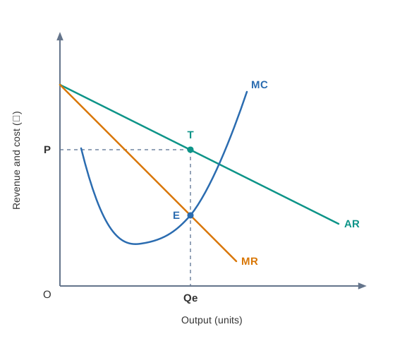
Fig. 8.21 – Producer’s equilibrium under imperfect competition.
The two approaches are the same proposition stated in two ways, and either may be asked for.
8.11 Summary
- Cost in economics is the value of the resources a firm gives up in producing a commodity. The word is used in three senses — what the firm has actually paid out, what it has forgone by using its own resources, and what production has cost society.
- Explicit cost, also called money cost or accounting cost, is the payment a firm makes to outsiders for the factor services it purchases or hires. It passes through the books of account and covers wages, materials, power, rent, interest and similar items.
- Implicit cost is the imputed value of the factor services a firm owns and uses in its own unit, measured by what those resources could have earned in their next best alternative use. No payment is made, so it is nowhere recorded.
- Normal profit is the minimum payment a producer must get to induce him to bear the risk of production. It is the supply price of entrepreneurial services and is therefore counted as a part of cost.
- Economic cost is the wider sense in which the economist takes cost, and it is the sense used in the theory of price.
- \(\text{Money cost} = \text{Accounting cost} = \text{Explicit cost}\), all in rupees for a given output and period.
- \(\text{Economic cost} = \text{Explicit cost} + \text{Implicit cost (including normal profit)}\), so economic cost is never smaller than accounting cost.
- Real cost refers to the efforts and sacrifices of the owners of the factors of production — the disutility of labour and the sacrifice involved in saving. It explains why factors must be paid, but being subjective it cannot be measured.
- Private cost is the economic cost borne by an individual firm, while social cost is what society bears on account of that production: \(\text{Social cost} = \text{Private cost} + \text{External cost}\), where external cost is the money value of the harm imposed on people outside the firm.
- Opportunity cost of producing a good is the value of the next best alternative given up in order to produce it, and it arises because resources are scarce and have alternative uses. Only the best of the alternatives forgone is counted, not all of them.
- Accounting cost records the payments actually made and covers explicit cost alone; opportunity cost measures the earning of the alternative surrendered and takes in implicit cost as well. Expressed in money, opportunity cost is the same thing as economic cost.
- In the short run at least one factor is fixed. Fixed factors cannot be increased or decreased whatever the output, while variable factors can be changed by any desired amount, and the two give rise to fixed cost and variable cost respectively.
- The three total costs of the short run are related by one equation, \(\text{TC} = \text{TFC} + \text{TVC}\), where TC is total cost, TFC total fixed cost and TVC total variable cost, all in rupees at the same output.
- Total fixed cost is the same at every output and has to be borne even at zero output, which is why it is called unavoidable or overhead cost.
- Total variable cost is zero at zero output and rises with output, first at a decreasing rate and then at an increasing rate.
- Since TFC is constant, every change in total cost is due entirely to the change in total variable cost.
- The total cost curves follow from this. The TFC curve is a horizontal straight line beginning on the Y-axis; the TVC curve is inverted S-shaped and begins at the origin; the TC curve has the same shape as TVC, begins on the Y-axis at the level of fixed cost, and stays parallel to TVC because the gap between them is the constant fixed cost.
- Average fixed cost is \(\text{AFC} = \dfrac{\text{TFC}}{Q}\), where TFC is total fixed cost in rupees and \(Q\) is output in units. It falls continuously as the constant overhead is spread over more units, and its curve is a rectangular hyperbola which approaches both axes without ever touching either.
- Average variable cost is \(\text{AVC} = \dfrac{\text{TVC}}{Q}\). It falls, reaches a minimum at the optimum capacity output and then rises, giving a U-shaped curve, and the U-shape follows from the law of variable proportions.
- Average total cost is \(\text{ATC} = \dfrac{\text{TC}}{Q} = \text{AFC} + \text{AVC}\), the per unit cost of all factors together.
- It is U-shaped, and its lowest point is the optimum point of production.
- Its minimum lies to the right of the minimum of AVC, because for a while the fall in AFC more than offsets the rise in AVC.
- The gap between ATC and AVC is AFC, so the two curves come closer as output rises but never meet.
- Marginal cost is the addition made to total cost by one more unit: \(\text{MC}_n = \text{TC}_n - \text{TC}_{n-1}\), or \(\text{MC} = \dfrac{\Delta \text{TC}}{\Delta Q}\), where \(\Delta \text{TC}\) is the change in total cost in rupees and \(\Delta Q\) the change in output.
- Marginal cost is unaffected by fixed cost and can equally be obtained from the total variable cost column.
- Total variable cost is the sum of the marginal costs of all the units produced, \(\text{TVC} = \Sigma \text{MC}\).
- The MC curve is U-shaped and reaches its minimum at a smaller output than either average curve.
- The relationship between average and marginal cost has three cases, and it concerns the direction in which average cost moves, not the direction in which marginal cost moves.
- When MC is less than AC, average cost falls.
- When MC is greater than AC, average cost rises.
- When MC equals AC, average cost is constant, and this happens at the minimum of the average cost curve, which the MC curve therefore cuts from below — both for AVC and for ATC.
- In the long run every factor, including the plant, is variable, so there is no fixed cost and only three curves remain — LTC, LAC and LMC. The LTC curve starts at the origin, since nothing is fixed and zero output costs nothing.
- Long-run average cost is the lowest per unit cost at which each output can be produced when the plant can be freely chosen. Its curve is the envelope, or planning curve, of the short-run average cost curves, touching each at one point and lying above none, and it is U-shaped but flatter than any of them. Long-run marginal cost bears the same relation to LAC that MC bears to AC, cutting it at its minimum point from below.
- The U-shape of the LAC curve is explained by economies and diseconomies of scale, not by the law of variable proportions.
- Internal economies arise from the growth of the firm’s own scale and are technical, managerial, marketing and financial; carried too far, expansion brings internal diseconomies of supervision and coordination.
- External economies arise from the growth of the industry as a whole, are shared by every firm in it, and shift the whole LAC curve downward, while external diseconomies shift it upward.
- Revenue means the receipts of a firm from the sale of its output, and is not to be confused with profit. Its three concepts are \(\text{TR} = P \times Q\), \(\text{AR} = \dfrac{\text{TR}}{Q} = P\) and \(\text{MR}_n = \text{TR}_n - \text{TR}_{n-1}\), where \(P\) is price in rupees per unit and \(Q\) the quantity sold; average revenue is the concept of revenue that is called price, and total revenue is also the sum of the marginal revenues, \(\text{TR} = \Sigma \text{MR}\).
- Under perfect competition the firm is a price-taker and sells any quantity at the ruling price, so \(\text{AR} = \text{MR} = P\). The AR and MR curves coincide in a single horizontal line, which is the perfectly elastic demand curve facing the firm, and the TR curve is an upward sloping straight line from the origin whose slope is the price.
- Under imperfect competition the firm must lower the price on all units in order to sell more.
- AR falls continuously but is never zero or negative; MR falls faster and lies below AR at every level of sales after the first unit.
- Where the AR curve is a straight line, MR falls at twice the rate of AR and bisects the perpendicular drawn from any point on AR to the Y-axis.
- MR may be positive, zero or negative, and the TR curve is dome-shaped, rising at a diminishing rate, reaching a maximum and then falling.
- The relationship between total and marginal revenue is that TR rises while MR is positive, is at its maximum where MR is zero, and falls once MR is negative.
- A producer is in equilibrium at the output that yields him the maximum profit, where \(\text{Profit} = \text{TR} - \text{TC}\) in rupees for the same output and period, and where he has no tendency to change what he produces.
- By the TR–TC approach, equilibrium is at the output at which the vertical gap between total revenue and total cost is the greatest, total revenue being above total cost.
- By the MR–MC approach, two conditions must hold together: marginal revenue must equal marginal cost, and marginal cost must be rising, so that it cuts the marginal revenue curve from below.
8.12 Points to Ponder
- Normal profit is treated as a part of the cost of production, so a firm whose total revenue exactly covers its economic cost is said to be earning no profit at all, and yet it stays in business. Is it sound to count a payment to the owner of the firm as a cost in the same way as the wages of a worker? What is lost, and what is gained, by the accountant’s practice of treating it instead as a surplus?
- A firm decides its output on private cost, while the true burden on the community is social cost. If a producer is made to bear a part of the external cost through a tax or an effluent standard, his costs rise, his output falls and some small units may close; if he is not, the commodity is produced in larger quantity than the community would choose. Where would you place the balance, and on what would your answer depend?
- Two shopkeepers with identical sales, one owning his premises and one paying rent, show very different profits in their account books but the same economic cost. Does bringing implicit cost into the reckoning change what the first shopkeeper ought to do, or only how he should describe what he is doing? What decision, if any, would he take differently after reading this chapter?
- The long-run average cost curve is drawn U-shaped on the argument that expansion eventually brings diseconomies of scale. Yet in some kinds of production a larger plant appears to be cheaper per unit however far it is extended, so that the curve would fall and never turn up. What would such a cost curve imply for the number of firms an industry could support, and for the buyer?
- The whole of this chapter rests on the assumption that a producer aims at the largest possible profit. A cooperative, a family workshop and a public sector enterprise may weigh employment, the interest of members or the availability of a service alongside profit. Does the rule that output should be carried to the point where marginal revenue equals marginal cost still guide such a producer, and if so, what has to be changed in it?
- Fixed cost has already been committed and cannot be escaped in the short run, whatever the firm now decides to produce. Should a producer therefore leave fixed cost entirely out of account when he settles this month’s output? If your answer is yes, what part can fixed cost still play in a decision, and when does it become relevant again?
8.13 Objective Questions
- Which of the following is an implicit cost of a firm? [1]
- Wages paid to casual workers
- Interest on capital borrowed from a bank
- Rent of a building owned by the entrepreneur and used in his own unit
- Insurance premium paid on the factory
- State whether the following statement is true or false: under perfect competition the average revenue and the marginal revenue of a firm are equal at every level of output. [1]
- Read the two statements below and choose the correct option. [1] Assertion (A): The marginal cost curve cuts the average total cost curve at the lowest point of the average total cost curve. Reason (R): Average cost falls so long as marginal cost lies below it and rises once marginal cost lies above it.
- Both Assertion (A) and Reason (R) are true, and Reason (R) is the correct explanation of Assertion (A).
- Both Assertion (A) and Reason (R) are true, but Reason (R) is not the correct explanation of Assertion (A).
- Assertion (A) is true, but Reason (R) is false.
- Assertion (A) is false, but Reason (R) is true.
- Fill in the blank: under imperfect competition, total revenue is at its maximum at the level of sales at which marginal revenue is ______. [1]
- Match each item in Column I with the item that describes it in Column II. [1]
| Column I | Column II |
|---|---|
| a. Average fixed cost curve | i. Arise from the expansion of the industry as a whole |
| b. Normal profit | ii. The minimum payment that induces an entrepreneur to bear the risk of production |
| c. External economies | iii. A rectangular hyperbola which touches neither axis |
8.14 Check Your Concepts
- Distinguish between explicit cost and implicit cost, giving one example of each. [2]
- The total cost of a firm is ₹320 when it produces 5 units and ₹372 when it produces 6 units, and its total fixed cost is ₹120. Calculate its average fixed cost, its average variable cost and its marginal cost at 6 units of output. [3]
- Draw the average variable cost curve and the average total cost curve of a firm in a single diagram and explain their relationship. Why does the gap between the two curves narrow as output rises without ever closing, and why does the average total cost curve reach its lowest point at a larger output than the average variable cost curve? [4]
- Compare the behaviour of average revenue and marginal revenue of a firm under perfect competition with their behaviour under imperfect competition. Support your answer with a diagram for each case, and explain why marginal revenue is less than average revenue in the second case. [6]
8.15 Case-Based Question
- Meera Kulkarni owns Sahyadri Packaging, a small unit making corrugated cartons which it sells in a competitive market at ₹120 a box, a price the unit is far too small to influence. Its fixed costs — the rent of the shed, interest on the loan taken for the cutting machine and the salaries of two permanent staff — come to ₹36,000 a month. The marginal cost of successive batches of 100 boxes has been ₹90, ₹100, ₹110, ₹120 and ₹135 a box. Meera works full time in the unit and draws no salary from it, although a larger firm has offered her ₹30,000 a month.
- State the batch up to which Sahyadri Packaging should produce, and give the two conditions of producer’s equilibrium that support your answer. [2]
- Identify one implicit cost of the unit from the passage, and explain how counting it changes the cost of production of Sahyadri Packaging. [2]