Chapter 10: Producer’s Equilibrium
Every producer must answer one question the moment production begins: how much to produce. Resources are scarce, so each extra unit of output draws in factor services that have alternative uses, and it adds to cost. Each extra unit also adds to revenue when it is sold. Whether that unit is worth producing depends on which of the two additions is larger. A knitwear unit in Tiruppur able to stitch anywhere between five hundred and five thousand shirts a month cannot choose among these levels freely. Beyond a point, overtime wages, machine strain and dearer inputs push the cost of one more shirt above the price it fetches, and total profit begins to fall. The output the producer finally settles at is the one it has no reason to move away from in either direction. That output is the producer’s equilibrium. This chapter explains what a firm is, why economics assumes that firms aim at maximum profit, and how the equilibrium level of output is located by the total revenue and total cost approach and by the marginal revenue and marginal cost approach.
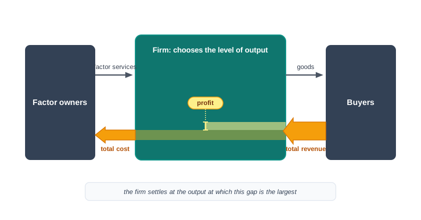
Fig. 10.0 – The firm between its costs and its revenue.
10.1 The Firm as an Economic Entity
Economic activity begins with a constraint. The resources of an economy are scarce, while the wants they are used to satisfy are unlimited. Goods and services must therefore be produced deliberately — in chosen quantities, by chosen methods, out of resources that could have been put to some other use.
The unit that takes those decisions is the producer. In economics the words producer, supplier and firm are used interchangeably. A firm may be one person working alone or an organisation employing thousands, but its economic character is the same in both cases: it hires factor services, turns them into goods and services, and sells what it produces to others.
This section explains what a firm is and what it does. The rest of the chapter asks the harder question — how the firm decides how much to produce.
10.1.1 Meaning of a Firm
A firm is an economic entity that employs factors of production to produce commodities which it sells to other people. Three parts of that statement carry weight. It employs factors, so it is a buyer in the factor market. It produces commodities, so it is a technical unit that transforms inputs into output. It sells what it produces, so production meant only for one’s own use falls outside the term.
The third part is what separates a firm from a household. A household that grows vegetables for its own kitchen does produce, but it sells nothing and earns no revenue, and so it is not producing as a firm. What induces a firm to produce for others is the expectation of profit, and it is this motive on which the whole of this chapter is built.
10.1.2 Functions of a Firm in the Economy
The firm is the basic production unit of an economy. It performs two functions, and the two together explain why it stands at the centre of economic activity.
- Buying factor services — the firm hires land, labour, capital and enterprise, largely from households and partly from other business entities, and pays rent, wages, interest and profit in return. Firms are therefore the principal buyers in the factor market, and the payments they make become the incomes out of which households buy goods.
- Transforming inputs into output — the firm combines the factor services it has hired and converts them into goods and services, which it then sells in the product market. Deciding what to produce, in what quantity, by what method and at what price is part of this second function.
- Some firms produce goods — food, cloth, cement, automobiles.
- Others produce services — transport, banking, insurance, repair work.
Firms are thus the main producers of commodities and, at the same time, the principal buyers of factor services. Every decision about output that this chapter examines is a decision taken inside this second function.
10.1.3 Nature and Types of Firms
Firms differ widely in what they produce, in how large they are and in how they are owned. Some are very small — a grocery shop, a vegetable stall, a bakery, a restaurant. Others are very large, employing thousands of workers and operating several plants. By ownership, a firm may be a sole proprietorship, a partnership or a company.
These differences matter to the accountant and to the law, but not to the theory of the firm. Whatever its size or legal form, every firm receives revenue from the sale of its output and incurs cost on the factors it employs, and every firm must settle on some level of output. That is why one set of rules, developed in this chapter, applies to all of them.
One distinction should be kept clear from the start. A firm is a single producing unit; an industry is the whole group of firms producing the same commodity. The cement industry is made up of many cement firms, and it is the individual firm whose behaviour is studied here.
10.2 Meaning of Producer’s Equilibrium
A firm that can produce any quantity between very little and a great deal must stop somewhere. The question this chapter answers is where, and why there rather than anywhere else. The answer is given by the idea of equilibrium, which economics has already used once, in explaining the behaviour of the consumer.
10.2.1 Equilibrium as a State of Rest
Equilibrium means a state of rest. It is the position in which the forces working in opposite directions are exactly in balance, so that there is no tendency left to move in either direction. The word says nothing about whether the position is large or small, good or bad. It says only that, in the given circumstances, there is no reason to move away from it.
In the theory of consumer behaviour the opposing forces were the satisfaction gained from one more unit and the price paid for it. For a producer the opposing forces are of the same shape: one more unit of output adds something to revenue and adds something to cost. So long as the two pulls are unequal, the firm has a reason to expand output or to contract it. When they no longer pull against each other, the firm rests.
10.2.2 Equilibrium of the Firm Defined
A firm is said to be in equilibrium when it selects that level of output at which it would like to stay, having no incentive to increase or decrease production from that level. Since the firm is assumed to be after profit, this rest position is reached where profit is as large as it can be made.
Four things in this definition should be noticed.
- Equilibrium is defined with reference to output — it is a level of production the firm settles at, not a price it announces or a profit figure it hopes for.
- The test is the absence of any incentive to change — if the firm could add to its profit by producing one unit more or one unit less, it is not yet in equilibrium.
- Demand conditions are given — they fix the revenue the firm can earn from its output, and under perfect competition they fix the price the firm must accept.
- Cost conditions are given — they fix what each level of output costs to produce. If either set of conditions changes, the old output ceases to be an equilibrium and a new one has to be found.
Producer’s equilibrium, or the equilibrium of the firm, can be shown in two ways. One works with the totals, comparing total revenue with total cost. The other works at the margin, comparing the revenue and the cost of one more unit. The two are complementary rather than rival: they use different measurements of the same information and always identify the same level of output. Sections 10.4 and 10.5 take them in turn.
10.3 The Objective of Profit Maximisation
Equilibrium was defined as the output at which profit is maximum. That definition rests on an assumption — that the firm wants the largest profit it can get, and wants nothing else more. Before the equilibrium output can be located, the assumption itself has to be examined, and the word ‘profit’ has to be given a meaning precise enough to be maximised.
10.3.1 Why Profit Maximisation Is Assumed
Economists take it that business firms always attempt to maximise their profits, or, where profit is impossible, to minimise their losses. They are perfectly aware that businessmen speak of other goals as well — larger sales, a faster growth rate, a bigger share of the market, sheer survival, a quiet life, generous salaries for the staff. A firm that has all these in view is not the single-minded profit maximiser of the textbook.
The assumption is nevertheless retained, for two reasons.
- Firms come fairly close to it in practice — an enterprise that neglects profit for long cannot pay its factors, cannot replace its equipment and cannot survive, so even firms pursuing other goals are held near the profit-maximising line by the discipline of cost.
- It predicts behaviour well — assuming profit maximisation, the theory forecasts how much a firm will produce and what price it will charge with reasonable accuracy, and a simple assumption that predicts correctly is worth more to analysis than a complicated one that does not.
For these reasons the whole traditional theory of price is built on the profit-maximisation hypothesis. Note also that the assumption covers bad times as well as good: when losses cannot be avoided, maximising profit means making the loss as small as possible.
10.3.2 Meaning of Profit
Profit is the surplus left with the firm out of what it earns after it has met what it spends. It compares two totals belonging to the same period and the same level of output: the revenue earned from selling that output, and the cost of producing it.
\[\pi = TR - TC\]
Here \(\pi\), the Greek letter pi, stands for total profit, \(TR\) for total revenue and \(TC\) for total cost, all three measured in rupees for a stated period of production. A positive value means the firm has earned a profit, a negative value means it has made a loss, and a zero value means revenue and cost are exactly matched.
Since \(TR\) and \(TC\) both rise as output rises, profit is not read off either curve alone but off the distance between them. Profit maximisation therefore means producing that level of output at which the excess of total revenue over total cost is the largest. This is the idea that Section 10.4 turns into a diagram.
The same magnitude can be reached through per unit figures. Revenue per unit is average revenue and cost per unit is average cost, so profit per unit is \(AR - AC\), and total profit is that margin multiplied by the number of units sold.
\[\pi = (AR - AC) \times Q\]
Here \(AR\) is average revenue in ₹ per unit, \(AC\) is average cost in ₹ per unit and \(Q\) is the quantity of output. What the firm maximises is \(\pi\), the product of the two terms — not the margin \(AR - AC\) by itself. A wide margin earned on a very small output can yield less total profit than a narrow margin earned on a large one.
10.3.3 Normal Profit
An entrepreneur who puts capital and effort into one line of production gives up what the same capital and effort could have earned elsewhere. Unless the business returns at least that much, it is not worth carrying on. This minimum return is called normal profit.
Normal profit is the pure return on capital together with the risk premium needed to compensate the entrepreneur for the risks of production. Because it equals the opportunity cost of the entrepreneur — the reward forgone in the next best use of the same resources — it is treated as a part of the cost of production and is included in total cost. This is one of the points at which the economist’s cost differs from the accountant’s.
10.3.4 Pure or Economic Profit
Once normal profit has been counted as a cost, anything the firm earns above total cost is a genuine surplus.
It follows that if revenue just equals cost, the firm is earning normal profit only; and if revenue exceeds cost, the firm is earning pure or economic profit in addition. Pure profit is the figure that guides the movement of resources in an economy. Positive pure profits in a line of production draw resource owners towards it in the hope of the same return, while losses — negative profits — push resources out of it into uses where they are better rewarded. In this sense pure profit performs the allocative work that the price mechanism relies on.
The two kinds of profit differ in what they measure and in what they do, and the main points of difference are set out below.
10.4 Producer’s Equilibrium: Total Revenue and Total Cost Approach
Profit was defined as the excess of total revenue over total cost. The most direct way of finding the profit-maximising output, therefore, is to set the two totals side by side at every level of output and look for the level at which the excess is the largest. This is the total revenue and total cost approach, and because it works with figures that a producer keeps anyway, it is the approach businessmen use most readily.
The whole method rests on one sentence: profit is maximum where \(TR - TC\) is maximum. Everything that follows is a way of locating that output on a diagram.
10.4.1 Behaviour of the Total Revenue and Total Cost Curves
The two curves have to be drawn before they can be compared, and each has a shape of its own.
Total revenue is the amount the firm earns from selling its output, so \(TR = P \times Q\). Under perfect competition the firm is a price taker: it sells every unit at the same given price, however much it produces. Total revenue therefore rises at a constant rate in direct proportion to output, and the TR curve is a straight line starting from the origin — at zero output nothing is sold and nothing is earned. Under imperfect competition, where the firm must lower price to sell more, the TR curve is not a straight line, but the rules of equilibrium set out here apply to that case as well.
Total cost behaves differently. At zero output the firm still bears its fixed costs, so the TC curve does not begin at the origin but at a point on the Y-axis equal to total fixed cost. It then rises throughout, since more output needs more variable inputs. Its shape follows the law of variable proportions: cost first increases at a decreasing rate, which makes the curve concave downward, and later increases at an increasing rate, which makes it concave upward. The two curves are drawn together in Fig. 10.1.
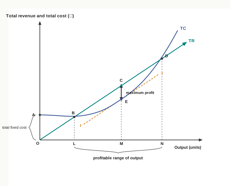
Fig. 10.1 – Profit maximisation by the total revenue and total cost approach.
10.4.2 Break-Even Point and the Profitable Range of Output
Read Fig. 10.1 from left to right. Up to output OL the TC curve lies above the TR curve. Cost exceeds revenue, and the firm is making losses equal to the vertical distance between the two curves. At OL the curves meet at point B: total revenue exactly equals total cost, and the firm makes neither profit nor loss. Point B is the break-even point.
Beyond OL the TR curve lies above the TC curve, and the firm earns profit at every level of output until ON is reached. At ON the curves meet again at D, and beyond ON total cost overtakes total revenue, so losses appear once more. The firm will therefore never choose to produce less than OL or more than ON, and the stretch between them is called the profitable range of output.
10.4.3 Determination of the Equilibrium Level of Output
Within the profitable range the firm earns profit at every output, but not the same profit. The distance between TR and TC first widens and then narrows, which means total profit first rises with output and later falls. Equilibrium is at the output where that distance is greatest.
In Fig. 10.1 the greatest vertical distance between the two curves is CE, which stands above output OM. At OM the firm earns the maximum profit it can earn, given the demand and cost conditions it faces, and any movement away from OM in either direction narrows the gap and reduces profit. OM is therefore the equilibrium level of output.
The point can be put more sharply. The gap between two rising curves is widest where they are rising at the same rate — that is, where their slopes are equal. This is why the tangent tt drawn to TC at E is parallel to TR. The slope of the TR curve is the addition made to revenue by one more unit, and the slope of the TC curve is the addition made to cost by one more unit. Equal slopes therefore mean that the last unit produced adds as much to cost as it adds to revenue, which is exactly the condition Section 10.5 arrives at from the other direction.
Two conditions summarise the approach.
- Total revenue must exceed total cost, so that the firm is inside its profitable range.
- The difference between total revenue and total cost must be the largest attainable, so that no change in output can add to profit.
10.4.4 The Total Profit Curve
The same result can be shown in one curve instead of two. Total profit at each level of output is the vertical distance between TR and TC, and plotting that distance against output gives the total profit curve, written TP. It is drawn in Fig. 10.2.
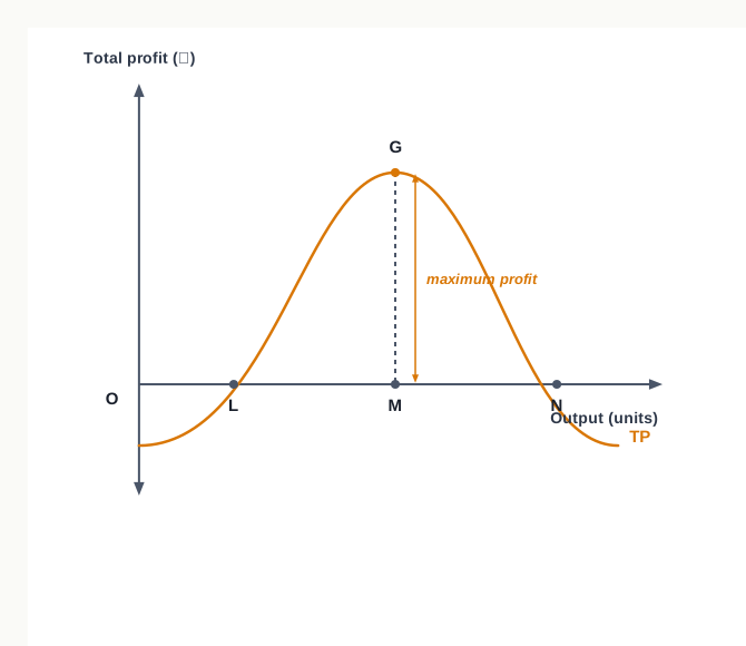
Fig. 10.2 – The total profit curve.
Up to OL the TP curve lies below the X-axis, because the firm is making losses there. At L it cuts the axis, since profit at the break-even output is zero. It then slopes upward, showing profit rising with output, until it reaches its highest point G above output OM. Beyond OM it slopes downward, showing profit falling, and at N it cuts the axis again. The peak of the TP curve and the widest gap in Fig. 10.1 identify the same output — OM — so the two figures tell one story in two ways.
10.4.5 Limitations of the Approach
The total revenue and total cost method is reasonable and is often employed by businessmen, but it has drawbacks as a tool of analysis.
- The maximum vertical distance between two curved lines cannot be judged at a glance, so the equilibrium output is hard to read off the diagram with any accuracy.
- Price per unit is not shown anywhere in the diagram, since the curves carry totals only, and much of the reasoning about a firm’s behaviour needs per unit figures.
- The approach reports the outcome of a decision rather than the decision itself — a producer does not compare whole totals afresh each morning, but asks whether one more unit is worth producing.
Each of these limitations points the same way: towards an approach that works at the margin. That is the subject of Section 10.5.
10.5 Producer’s Equilibrium: Marginal Revenue and Marginal Cost Approach
A producer does not weigh whole totals afresh every morning. The decision actually taken is a smaller one, taken again and again: is it worth producing one more unit? That question is answered by comparing what the extra unit adds to revenue with what it adds to cost. The addition made to total revenue by selling one more unit is marginal revenue, and the addition made to total cost by producing it is marginal cost.
This is the second and more popular approach to the equilibrium of the firm. Three rules have to be satisfied before profit can be said to be at its maximum: a rule about whether to produce at all, a rule that is necessary for profit to be maximum, and a rule that ensures profit is being maximised rather than minimised. They are taken in turn.
10.5.1 Whether to Produce at All in the Short Run
In the short run some costs are fixed. Rent on the premises, interest on borrowed capital and the salaries of permanent staff have to be met whether the machines run or stand idle. It is these fixed costs that explain why a firm sometimes goes on producing even while it is making losses.
Suppose the firm closes down and produces nothing. Its revenue is then zero, but its fixed costs remain, so its loss is exactly equal to its total fixed cost. A firm that produces no output in order to keep its loss down is in a situation of shut-down. No profit-maximising firm will accept a loss larger than its fixed cost, since shutting down always caps the loss at that figure.
The comparison, then, is between the loss made while producing and the loss made while shut down.
- If price equals average variable cost — the firm covers its variable costs exactly and recovers nothing towards fixed cost, so its loss while producing is equal to fixed cost, the same as under shut-down. The two positions are equally bad.
- If price is greater than average variable cost — the firm covers all its variable cost and part of its fixed cost as well, so the loss while producing is smaller than fixed cost. Producing is the better of the two.
- If price is less than average variable cost — the firm cannot even meet the cost of the inputs it is currently using, so every unit produced adds to the loss. Shutting down is the better of the two.
10.5.2 The Necessary Condition: Marginal Cost Equals Marginal Revenue
Once Rule 1 is satisfied and the firm has decided that producing is worthwhile, the question becomes how much to produce. The answer follows from a simple comparison made unit by unit.
If marginal revenue exceeds marginal cost, the unit under consideration adds more to revenue than it adds to cost, so producing it adds to profit. The firm gains by expanding output. If marginal cost exceeds marginal revenue, that unit adds more to cost than to revenue and eats into profit. The firm gains by cutting output back.
So long as the two are unequal in either direction, the firm has a reason to change its output, and a position it has reason to leave is not equilibrium. Only when the addition to cost exactly matches the addition to revenue is there nothing to gain from producing either more or less.
10.5.3 The Sufficient Condition: Marginal Cost Cutting Marginal Revenue From Below
Rule 2 is necessary but it is not enough, because marginal cost can equal marginal revenue at more than one level of output — and at one of them profit is at its lowest, not its highest. Fig. 10.3 shows why.
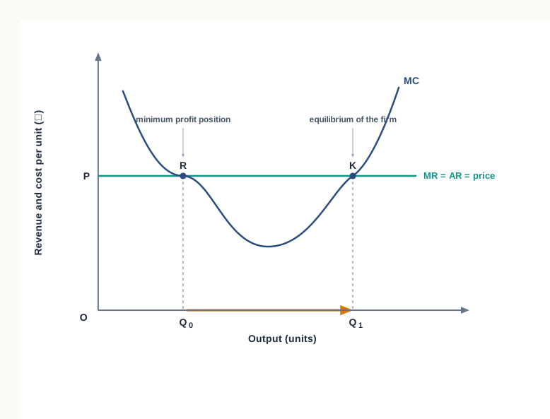
Fig. 10.3 – Equilibrium of the firm by the marginal revenue and marginal cost approach.
At output \(OQ_0\) the two are equal at point R, but the MC curve is falling and cuts the MR line from above. Just beyond \(OQ_0\) marginal cost lies below marginal revenue, so each further unit adds to profit and the firm has every reason to expand. A position the firm wants to move away from cannot be equilibrium; \(OQ_0\) is in fact the firm’s minimum profit position.
At output \(OQ_1\) the two are equal again at point K, but here the MC curve is rising and cuts the MR line from below. Just below \(OQ_1\) marginal cost is less than marginal revenue, so cutting output would sacrifice profit. Just above \(OQ_1\) marginal cost exceeds marginal revenue, so expanding output would add more to cost than to revenue. Movement in either direction reduces profit, and the firm rests. Point K is the equilibrium of the firm and \(OQ_1\) is its equilibrium output.
10.5.4 The Two Conditions Taken Together
The two conditions of Rules 2 and 3 are given standard names. \(MR = MC\) is the first order condition of profit maximisation, and a rising marginal cost curve cutting the marginal revenue curve from below is the second order condition. Neither is sufficient by itself; taken together they are necessary and sufficient for profit maximisation, or, where profit is not possible, for loss minimisation.
The result also agrees with the approach of Section 10.4, as it must, since both use the same information. Marginal revenue is the slope of the total revenue curve and marginal cost is the slope of the total cost curve. To say that \(MR = MC\) is to say that the two total curves are rising at the same rate, which is exactly where the gap between them is widest.
In a schedule the two marginal figures rarely come out exactly equal, so the working rule is to keep producing while marginal revenue is at least equal to marginal cost, and to stop at the last unit for which this holds. Table 10.2 sets out the marginal figures of the firm already met in Section 10.4.
10.6 Summary
- A firm is an economic entity which employs factors of production to produce commodities that it sells to other people. Production meant only for one’s own use is left out, and a firm must be distinguished from an industry, which is the whole group of firms producing the same commodity.
- A firm performs two functions in an economy.
- It buys factor services, largely from households, and pays rent, wages, interest and profit for them, so it is the principal buyer in the factor market.
- It transforms these inputs into goods and services and sells them, so it is the main seller in the product market.
- Equilibrium means a state of rest, in which the forces working in opposite directions are exactly in balance and there is no tendency to move either way.
- A firm is in equilibrium when, given the demand and cost conditions, it produces that level of output at which its profit is maximum. Equilibrium is defined with reference to output, and the test is that the firm has no incentive to produce either more or less.
- Traditional theory assumes profit maximisation as the sole objective of a firm, although businessmen also pursue sales, growth, market share and survival. The assumption is retained for two reasons.
- Firms come fairly close to acting as profit maximisers in practice, since a firm that neglects profit cannot survive.
- The assumption predicts the output and price behaviour of firms accurately.
- Profit is the excess of total revenue over total cost, written \(\pi = TR - TC\), where \(\pi\) is total profit, \(TR\) total revenue and \(TC\) total cost, all measured in rupees for a stated period. A positive value is profit, a negative value a loss.
- The same magnitude in per unit terms is \(\pi = (AR - AC) \times Q\), where \(AR\) is average revenue and \(AC\) average cost in ₹ per unit and \(Q\) is output. The firm maximises the total, not the per unit margin.
- Normal profit is that amount of profit which is high enough to keep existing firms in the industry and low enough not to attract new ones. It equals the opportunity cost of the entrepreneur and is included in the cost of production.
- Pure or economic profit, also called super-normal or abnormal profit, is the excess of revenue over cost after normal profit has been counted as a cost. Positive pure profit draws resources into an industry and losses drive them out, which is how profit guides the allocation of resources.
- Under the total revenue and total cost approach, the TR curve is a straight line from the origin when the firm sells at a given price, while the TC curve starts on the Y-axis at total fixed cost and rises, first at a decreasing rate and later at an increasing rate.
- The break-even point is the output at which total revenue exactly equals total cost. The two curves cut each other twice, and the stretch of output between the two break-even points is the profitable range.
- Equilibrium is at the output at which the vertical distance between TR and TC is the largest, that is, where total profit is maximum. At that output the slopes of the two curves are equal, which is the same as saying that marginal revenue equals marginal cost.
- The total profit curve TP plots the distance between TR and TC. It lies below the X-axis where the firm makes losses, cuts the axis at each break-even output, and reaches its peak at the equilibrium level of output.
- The approach has limitations: the widest gap between two curves cannot be judged at a glance, price per unit is not shown in the diagram, and it reports the outcome rather than the unit-by-unit decision the producer actually takes.
- Under the marginal revenue and marginal cost approach, three rules must be satisfied.
- Rule 1 — in the short run a firm should produce if and only if \(AR \geq AVC\), or \(TR \geq TVC\); below that, shutting down leaves the smaller loss, equal to fixed cost.
- Rule 2 — the necessary condition for profit maximisation is \(MR = MC\), since unequal marginal figures always leave a gain from changing output.
- Rule 3 — the sufficient condition is that MC must be less than MR at a slightly lower output and greater at a slightly higher one, that is, the MC curve must cut the MR curve from below.
- \(MR = MC\) is called the first order condition and a rising MC curve cutting MR from below the second order condition. Where MC cuts MR from above, the firm is at its minimum profit position, not at equilibrium.
- The two approaches use the same information in different measurements and always identify the same equilibrium output, as set out below.
10.7 Points to Ponder
- A firm that spends years building market share while earning very little may be sacrificing profit today for larger profit later. If that is so, is it a counter-example to the profit-maximisation assumption, or an illustration of it over a longer horizon — and what evidence would settle the question either way?
- The economist counts the entrepreneur’s opportunity cost as part of cost; the accountant does not. When a government decides whether a public enterprise is ‘running at a loss’, which of the two measures should it use, and what would follow from choosing the other?
- A firm that covers its variable cost but not its fixed cost goes on producing and goes on losing money. For how long can that decision be defended, and what exactly changes when the short run gives way to the long run?
- Pure profit is said to guide resources into the industries where they are most valued. What happens to that signal when entry into an industry is restricted by licensing, by very large capital requirements, or by control over a scarce raw material?
- Very few producers actually know the marginal cost of their next unit of output. Does the rule that a firm produces where marginal revenue equals marginal cost then describe how producers behave, or only explain after the event why the output they chose was the profitable one?
- Suppose the commodity is an essential one — electricity, or a life-saving medicine. Should the producer be expected to stop at the profit-maximising output? If it is asked to produce more than that, who bears the cost of the extra output, and for how long can that arrangement last?
10.8 Objective Questions
- Under the total revenue and total cost approach, a firm is in equilibrium at that level of output at which: [1]
- total revenue is maximum
- total cost is minimum
- the difference between total revenue and total cost is the largest
- total revenue is equal to total cost
- A firm producing under perfect competition is in equilibrium where: [1]
- marginal revenue equals marginal cost and the marginal cost curve cuts the marginal revenue curve from above
- marginal revenue equals marginal cost and the marginal cost curve cuts the marginal revenue curve from below
- marginal revenue is greater than marginal cost
- marginal revenue is at its maximum
- Given below are two statements marked as Assertion (A) and Reason (R). Read them carefully and choose the correct option. [1] Assertion (A): A firm may go on producing in the short run even while it is making a loss. Reason (R): In the short run fixed costs have to be borne whether or not any output is produced.
- Both (A) and (R) are true, and (R) is the correct explanation of (A).
- Both (A) and (R) are true, but (R) is not the correct explanation of (A).
- is true, but (R) is false.
- is false, but (R) is true.
- Profit which is just high enough to keep existing firms in the industry and just low enough not to attract new firms into it is called ____________ profit. [1]
- Match the situation in Column I with the position of the firm in Column II. [1]
| Column I | Column II |
|---|---|
| a. Total revenue is exactly equal to total cost | i. Shut-down situation |
| b. The falling marginal cost curve cuts the marginal revenue curve | ii. Minimum profit position |
| c. Price falls below average variable cost | iii. Break-even point |
10.9 Check Your Concepts
- What is meant by producer’s equilibrium? [2]
- Distinguish between normal profit and pure profit on any three bases. [3]
- A firm sells its output at a constant price of ₹10 per unit. Its total cost at outputs of 0, 1, 2, 3, 4, 5 and 6 units is ₹12, ₹19, ₹25, ₹30, ₹36, ₹44 and ₹56 respectively. Find the equilibrium level of output and the maximum profit earned, and state the break-even level of output. [4]
- Show with the help of a diagram that a firm is in equilibrium at the output at which marginal cost equals marginal revenue, and explain why this equality by itself is not enough for profit to be maximum. [6]
10.10 Case-Based Question
- Meera runs Sunrise Packaging, a small unit making corrugated boxes, and sells every box at ₹18 in a market where she has no influence over the price. Her records for the current month show that the 400th box added ₹18 to her revenue and ₹15 to her cost, while the 460th box would add ₹18 to her revenue and ₹21 to her cost. Her fixed costs come to ₹12,000 a month.
- Should Meera raise her output beyond 400 boxes? Give a reason for your answer. [2]
- Meera says she will keep the unit running next month even if she makes a loss. Under what condition would that decision be the correct one, and why? [2]