Chapter 11: Determination of Equilibrium Price and Output Under Perfect Competition
On a winter morning at a wholesale vegetable mandi, several hundred farmers arrive with the same grade of potato. No single farmer’s load is large enough to move the day’s price, and no single trader’s purchase is large enough either. Yet by mid-morning a price has been settled, and every lot changes hands at close to that figure. Nobody announced it, and nobody could have refused it. Perfect competition is the model economics uses to explain how such a price comes about. The market itself — the whole body of buyers and the whole body of sellers — fixes the price. The individual firm receives it as a fact and is left with one decision only: how much to produce at that price. Its answer depends on what an extra unit costs it, and on whether that price covers the cost. This chapter explains how the market price is determined under perfect competition, how a firm chooses its equilibrium output at that price, when it earns super-normal profits, normal profits or losses, when it shuts down, and why only normal profits survive in the long run.
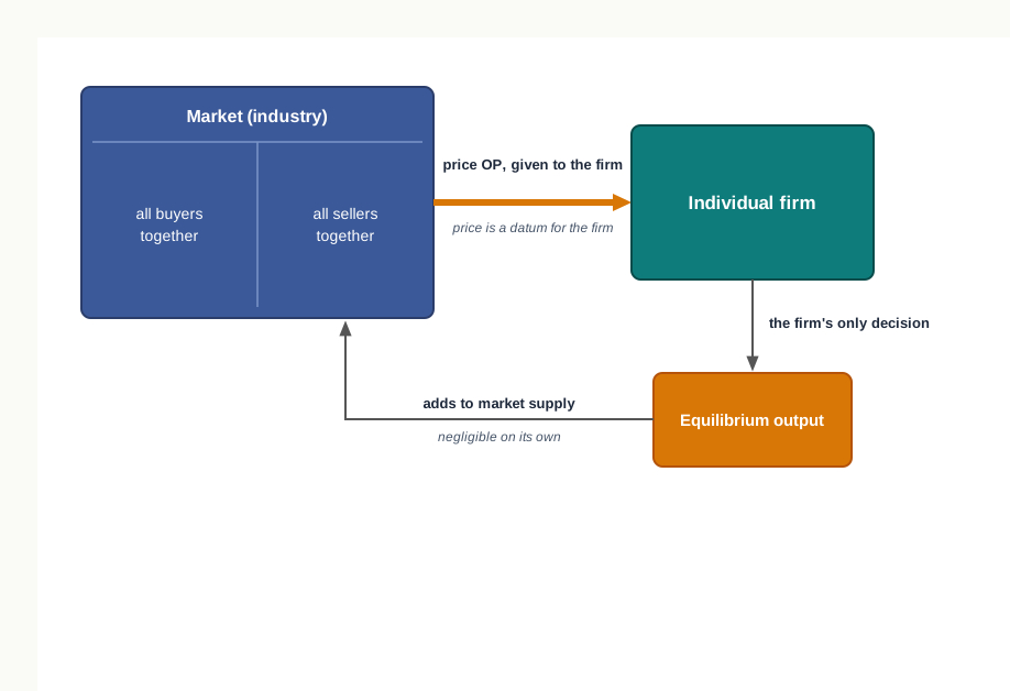
Fig. 11.0 – Price and output under perfect competition.
11.1 The Firm and the Industry Under Perfect Competition
Every market has to settle two things: the price at which the commodity will sell, and the quantity that will be produced. Under perfect competition these two questions are answered by two different bodies. The price is settled by the market as a whole, while the quantity is settled by each producer separately, taking that price as given.
The whole of this chapter rests on that division, so it must be made exact before anything else is attempted. Perfect competition is the market form in which a large number of buyers and a large number of sellers deal in a homogeneous product, with free entry and free exit and full knowledge of the ruling price. Its features were studied along with the other market forms, and are recalled here only so far as they bear on price and output.
- Large number of buyers and sellers — each one handles so small a share of the total that its own decision cannot move the market price.
- Homogeneous product — every seller’s unit is identical, so a buyer has no reason to pay one seller more than another.
- Free entry and free exit — firms may join the industry when it is profitable to do so and leave it when it is not.
- Perfect knowledge — buyers and sellers know the ruling price, so one price prevails throughout the market.
- Absence of selling costs — since the product is identical and the price is known, advertising cannot draw a buyer away from a rival.
The first two features together make the individual seller powerless over price. The third decides what happens to profits in the long run, and is taken up in Section 11.5.
11.1.1 Firm and Industry Distinguished
A firm is a single producing unit under one management, taking its own decisions about how much to produce. An industry is the group of all the firms producing a well-defined homogeneous product, and it is the industry, not the firm, whose supply meets the demand of all the buyers together.
The distinction matters because the two operate on different scales. What one firm produces is a negligible fraction of what the industry produces, and a fraction that small cannot alter the price at which the product sells. What all the firms produce together is the entire supply of the market, and that supply, set against the demand of all the buyers, is what fixes the price.
11.1.2 The Firm as a Price-Taker
Since the firm cannot influence the price, the price arrives as a datum, in the same way that the weather arrives for a farmer. Such a firm is described as a price-taker.
Two conditions of perfect competition make this position inescapable. Because the product is homogeneous and buyers know the ruling price, a firm that asks even a little more than the market price sells nothing at all — every buyer moves to a rival selling an identical unit. Because the firm’s own output is negligible, it can sell whatever it is able to produce at the ruling price, so it has no reason to ask for less. Its price is therefore fixed for it, above and below.
What is left to the firm is the quantity. It has to decide how much to produce at the given price so as to earn the largest profit it can, which is why a firm under perfect competition is called an output-adjuster.
11.1.3 Demand Curve of the Firm and the Equality of Price, AR and MR
If the firm can sell any quantity within its reach at the ruling price and nothing at all above it, the demand curve it faces must be a horizontal straight line drawn at that price. Demand for the firm’s product is therefore perfectly elastic, as shown in Fig. 11.1.
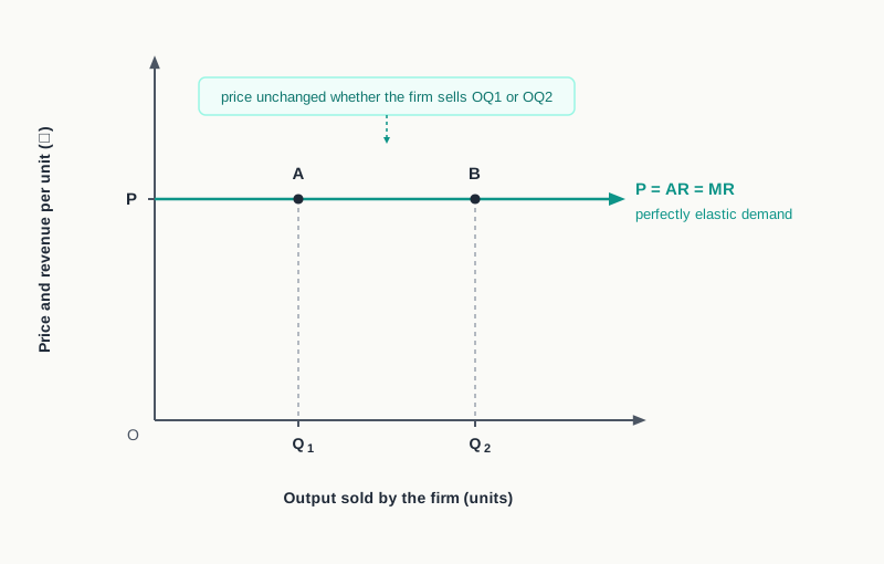
Fig. 11.1 – Demand curve faced by a firm under perfect competition.
This is the one point at which the firm’s demand curve differs from the market demand curve for the same commodity. The market curve slopes downward, because a lower price is needed to induce buyers as a body to take a larger quantity. The curve facing one firm within that market is flat, because the quantities that single firm can add to or withhold from the market are too small to call for any change in price at all.
The consequence for revenue follows at once. Total revenue is what the firm receives from selling its whole output, average revenue is what it receives per unit sold, and marginal revenue is the addition made to total revenue by selling one unit more.
\[AR = \dfrac{TR}{Q} \qquad MR = \dfrac{\Delta TR}{\Delta Q}\]
Here \(TR\) is total revenue in rupees, \(Q\) the number of units sold, \(\Delta TR\) the change in total revenue and \(\Delta Q\) the change in output, taken as one unit. Both \(AR\) and \(MR\) are measured in rupees per unit.
Because the price does not fall as the firm sells more, every additional unit adds exactly the price to total revenue. Average revenue is then the price itself, and marginal revenue is equal to it at every level of output. Table 11.1 sets this out for a firm facing a ruling price of ₹20 per unit.
The two revenue curves do not merely happen to be equal at one output. They coincide, and the single horizontal line at the ruling price is at once the demand curve of the firm, its average revenue curve and its marginal revenue curve. This is the relation \(P = AR = MR\), and every diagram of a competitive firm in this chapter carries it.
The main points on which the firm and the industry differ are set out below.
11.2 Determination of Price in the Market
The firm takes the price as given. The question left over is where that price comes from, and the answer is that it comes from the industry. All the buyers of the commodity together make up the market demand, all the firms in the industry together make up the market supply, and the price is whatever these two forces jointly permit. Neither side chooses it, and no single participant on either side is large enough to impose it.
11.2.1 Equilibrium of the Industry
The market demand curve slopes downward, since buyers as a body take a larger quantity only at a lower price. The market supply curve slopes upward, since a higher price makes it worth the industry’s while to offer more. There is one price at which the quantity buyers wish to take is exactly the quantity sellers wish to offer, and it is at that price alone that the market can come to rest.
The schedules in Table 11.2 show how this price is arrived at. The last column subtracts demand from supply, so a positive figure records a surplus in the market and a negative figure a shortage.
At ₹20 the two quantities are equal at 60 thousand units, and the last column reads zero. This is the equilibrium price, and 60 thousand units is the equilibrium quantity of the industry. At every other price in the schedule one side of the market is disappointed, and a disappointed buyer or seller acts on the price.
The same result is reached on a diagram by drawing the two curves together, as in Fig. 11.2. The price at which they intersect is then carried across to the individual firm, whose position was described in Section 11.1.
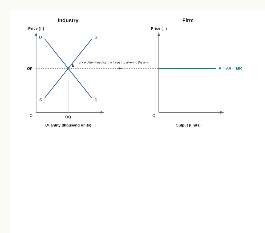
Fig. 11.2 – Determination of market price and the firm’s demand curve.
11.2.2 Excess Demand, Excess Supply and the Return to Equilibrium
A price other than OP does not survive, because it leaves one side of the market unsatisfied and that dissatisfaction acts on the price itself. The two cases are shown in Fig. 11.3.
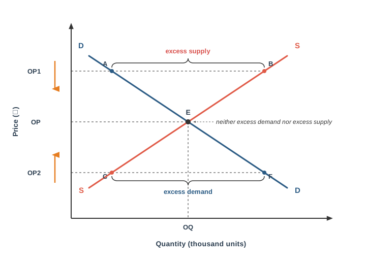
Fig. 11.3 – Excess supply and excess demand in the market.
At the higher price OP1, sellers offer AB more than buyers are willing to take. This surplus is excess supply. Stocks pile up unsold, and sellers who would rather part with the goods than hold them begin to accept less. The price is pushed down towards OP, and as it falls the quantity demanded expands along DD while the quantity supplied contracts along SS, until the gap closes.
At the lower price OP2, buyers want CF more than sellers are willing to offer. This shortage is excess demand. Buyers who cannot get the quantity they want compete against one another and offer more, and the price is pulled up towards OP. Once again the movement is along both curves, and it stops only when the two quantities are equal.
Only at OP is there neither a surplus to push the price down nor a shortage to pull it up. The market therefore settles there, and stays there so long as the curves themselves do not shift. It is this price that reaches the firm as a fact it cannot alter.
11.3 Short-Run Equilibrium of the Firm
The price has been settled by the industry and handed to the firm. The firm’s own problem now begins, and it is a problem of choice under a constraint: the price is fixed, the plant is fixed, and only the quantity produced can be varied. The firm has to pick the output at which the gap between what it earns and what it spends is as wide as it can be made.
In the short run some factors cannot be varied, so the firm carries a fixed cost whatever it produces. Its short-run cost curves are written SMC for short-run marginal cost, SAC for short-run average cost and AVC for average variable cost, and they take the usual U-shaped form.
11.3.1 Conditions of Short-Run Equilibrium
The firm reasons at the margin. If an extra unit adds more to revenue than it adds to cost, that unit is worth producing and profit rises. If it adds more to cost than to revenue, producing it eats into profit. Output should therefore be pushed to the point at which the two additions are equal, and no further.
- Marginal cost equals marginal revenue — the firm expands output while \(MR > MC\) and contracts it while \(MC > MR\), so profit is largest where \(SMC = MR\). Since price, average revenue and marginal revenue are the same figure for a competitive firm, this condition can also be written \(SMC = P\), and it is called the profit-maximisation rule.
- Marginal cost is rising at that output — the SMC curve must cut the MR line from below. Where SMC falls through the MR line, each further unit still costs less than it earns, so profit has not yet been exhausted and the point cannot be an equilibrium.
The first condition alone does not tell us whether the firm is prospering. That depends on how the price compares with average cost, and in the short run all three possibilities are open. Where \(AR > SAC\) the firm earns super-normal profits, where \(AR = SAC\) it earns normal profits only, and where \(AR < SAC\) it makes a loss. All three are genuine equilibrium positions, provided price at least covers average variable cost.
Since normal profit is already inside the cost curves, a firm at \(AR = SAC\) is not working for nothing. It is earning precisely what it needs to remain in the industry, and anything above that is super-normal profit.
The three positions are worked out below from a single cost schedule. Table 11.3 gives the short-run costs of a firm whose fixed cost is ₹20, and the working for both solved examples is drawn from it.
11.3.2 Equilibrium with Super-Normal Profits
If the ruling price stands above the lowest point of the SAC curve, there is a range of output over which each unit sells for more than it costs on average. The firm settles where marginal cost has risen to meet the price, and at that output average revenue is above average cost.
The same position is shown on a diagram in Fig. 11.4, where the per-unit profit is the vertical distance between the price line and the SAC curve at the equilibrium output, and total profit is that distance multiplied by the output.
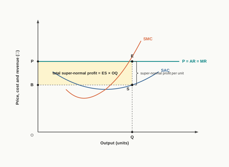
Fig. 11.4 – Short-run equilibrium of a firm earning super-normal profits.
11.3.3 Equilibrium with Normal Profits
Suppose the price is exactly equal to the lowest average cost the firm can achieve. Then the price line touches the SAC curve at one point only, and that point is also where SMC cuts the price line. In Table 11.3 this happens at a price of ₹16: the firm produces 5 units, earns \(TR = \text{₹}80\) and incurs \(TC = \text{₹}80\), so average revenue and average cost are both ₹16.
The firm here is exactly covering its total cost, including the normal profit contained in it. It has no surplus above what it must earn to stay in business, but it is losing nothing either. Fig. 11.5 shows the price line as a tangent to the SAC curve at its minimum point.
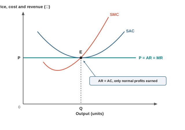
Fig. 11.5 – Short-run equilibrium of a firm earning normal profits.
11.3.4 Equilibrium with Losses
If the price falls below the lowest point of the SAC curve, no output can cover average cost and a loss is unavoidable. The firm’s choice is then between two losses, not between profit and loss, and the marginal rule still applies: it selects the output at which SMC has risen to the price, because that output makes the loss as small as it can be made.
The reasoning in the last step is the key to loss-making in the short run. Fixed cost has to be met whether the plant works or not, so a price that covers average variable cost and leaves something over is worth accepting: the surplus over variable cost goes towards the fixed burden and reduces the loss. Fig. 11.6 shows this position, with the price line below SAC but still above AVC.
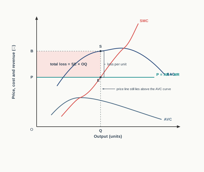
Fig. 11.6 – Short-run equilibrium of a firm incurring losses.
In all three cases the firm is in equilibrium in the same sense: given the price and its cost conditions, there is no output it would rather produce. What differs is only the level at which the price line happens to lie against the average cost curve.
11.4 Shut-Down Point, Break-Even Point and the Supply Curve of the Firm
A loss-making firm was seen to go on producing because the price still covered its running costs. That answer holds only up to a point, and the obvious question is where the point lies. Two prices mark out the firm’s position in the short run: the price at which it just covers its variable cost, and the price at which it just covers the whole of its cost. Between them the firm works at a loss but is right to work; below the first it is right to stop.
11.4.1 Shut-Down Point
Fixed cost is a burden the firm carries whether the plant runs or lies idle. It is therefore irrelevant to the decision whether to run: what matters is whether the price covers the cost the firm incurs only by producing, that is, its variable cost. So long as price is above average variable cost, every unit sold leaves a margin over its own running cost, and that margin goes towards the fixed burden. When price falls to average variable cost, the margin disappears and the firm is working merely to lose its fixed cost, exactly what it would lose by closing. Below that price, working makes the loss larger than closing would.
The lowest point of the AVC curve is thus the last position at which production is worth undertaking, and it is called the shut-down point.
Fig. 11.7 shows the shut-down point together with the price at which the firm covers all its costs, taken up next.
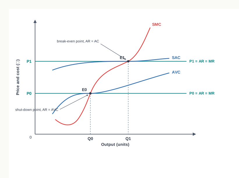
Fig. 11.7 – Shut-down point and break-even point.
11.4.2 Break-Even Point
At the other end of the loss range is the price at which the firm covers everything: its variable cost, its fixed cost and the normal profit contained in average cost. Since the firm can do no better than its lowest average cost, this happens at the minimum point of the SAC curve, which is also the point at which SMC cuts SAC. This is the break-even point, marked E1 in Fig. 11.7.
Both prices can be read off a cost schedule. The working for the firm of Table 11.3 is set out in Table 11.4.
The two points are often confused because both are read off the cost curves at their minimum points. The main points of difference are set out below.
11.4.3 Derivation of the Short-Run Supply Curve
The supply curve of a firm shows the quantity it is willing to offer at each price. That quantity has already been found: at any price the firm produces the output at which SMC has risen to meet the price, provided the price is not below average variable cost. Every price therefore yields one equilibrium output, and joining these price–quantity combinations gives the firm’s supply curve, as in Fig. 11.8.
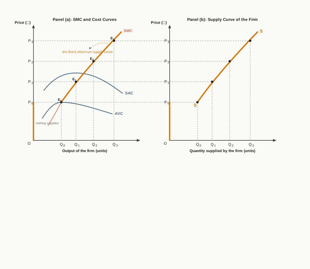
Fig. 11.8 – Derivation of the short-run supply curve.
Two features of the curve follow from the way it was obtained. It begins at the shut-down point, because at any price below P0 the firm offers nothing at all. And it slopes upward, because the relevant stretch of the SMC curve is its rising stretch: marginal cost increases as output is pushed up in a fixed plant, so a higher price is needed to make a larger output worth producing.
That part of the short-run marginal cost curve which lies above the minimum point of the average variable cost curve is therefore the supply curve of the firm in the short run.
This completes the circle begun in Section 11.2. The market supply curve SS, which met the market demand curve and fixed the price, is nothing but the supply curves of all the individual firms added together at each price. The industry hands the price down to the firm, and the firms’ own cost conditions build the supply that helped determine it.
11.5 Long-Run Equilibrium Under Perfect Competition
Two things were held fixed in the short run: the size of the plant, and the number of firms in the industry. The long run releases both. Every factor becomes variable, so a firm may build a larger or smaller plant, and there is time enough for new firms to be set up and for existing firms to wind up their business and leave.
The second of these matters more for price. Once the number of firms can change, the industry’s supply is no longer fixed by the firms that happen to be present, and the profits or losses of the short run become a signal that alters that number.
11.5.1 Free Entry and Free Exit
Suppose the firms in an industry are earning super-normal profits. That is an invitation to resource owners outside it, since the same resources are earning less elsewhere. New firms are set up, the industry’s supply increases, and the market supply curve shifts to the right. With the market demand curve unchanged, the equilibrium price falls. As it falls, the super-normal profits of every firm are squeezed, and entry goes on until there is nothing left to attract a newcomer, that is, until only normal profits remain.
The reverse works just as surely. If firms are making losses, some of them wind up and leave the industry. Supply contracts, the market supply curve shifts to the left, and the price rises. Losses shrink as it rises, and exit continues until the firms that remain are covering their costs in full. Both movements are shown in Fig. 11.9.
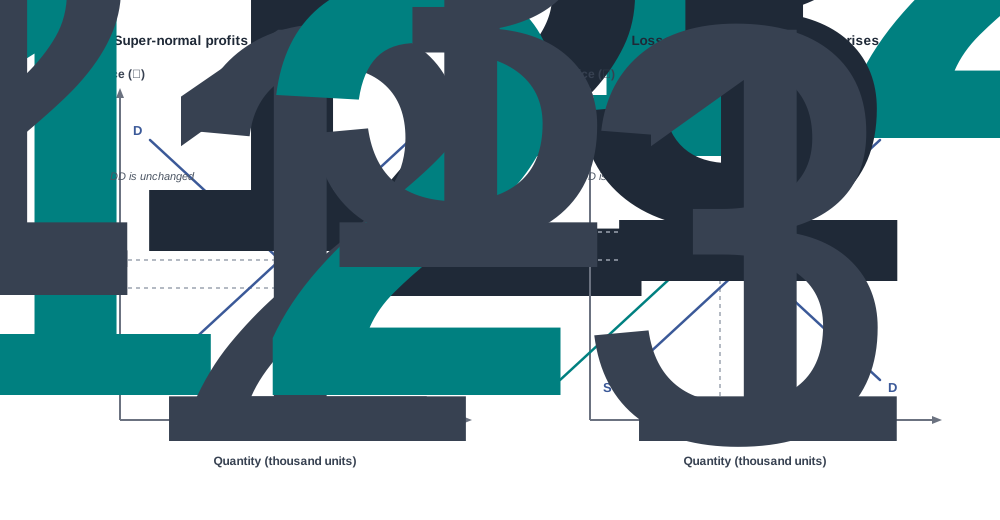
Fig. 11.9 – How entry and exit restore normal profits.
Free entry and free exit are therefore not decorative features of the model. They are the mechanism by which the industry’s price is dragged to the level of the firms’ costs, and they are the reason a competitive firm cannot hold on to abnormal profits however efficient it is.
11.5.2 Long-Run Equilibrium of the Firm
A firm is in long-run equilibrium when it has no reason to change its output, no reason to change the size of its plant, and no reason to leave the industry, while no outsider has any reason to enter. Two conditions express this.
- Long-run marginal cost equals marginal revenue — the profit-maximisation rule holds in the long run as it did in the short run, so \(LMC = MR\), and the LMC curve must cut the MR line from below.
- Average revenue equals long-run average cost — the firm earns normal profits only, since anything more would draw fresh firms in and anything less would drive some firms out.
Since price, average revenue and marginal revenue are one and the same figure for a competitive firm, the two conditions can be written as a single chain.
\[LMC = MR = AR = LAC\]
Here \(LMC\) is long-run marginal cost, \(LAC\) long-run average cost, \(MR\) marginal revenue and \(AR\) average revenue, each measured in rupees per unit, and all four are equal to the ruling price at the equilibrium output.
The chain carries a further consequence. Marginal cost can be equal to average cost only where average cost is at its lowest, since marginal cost pulls average cost down while it lies below it and pushes it up once it rises above it. A firm in long-run equilibrium is therefore producing at the minimum point of its LAC curve, which is its optimum output.
This result is why perfect competition is used as a standard of efficiency against which other market forms are judged. The consumer pays a price equal to the lowest average cost at which the good can be made, and no firm in the industry has the room to charge more or the incentive to produce at any other scale.
The way equilibrium in the two periods differs is set out below.
11.5.3 Long-Run Equilibrium of the Industry
The industry is at rest only when nothing in it is any longer changing: neither the price, nor the number of firms. Two conditions have to hold together.
- Market demand equals market supply — the price stands where the market demand curve cuts the market supply curve, so there is neither excess demand to raise it nor excess supply to lower it.
- The industry is neither expanding nor contracting — no firm is entering and none is leaving, which can only be the case when every firm in the industry is earning normal profits at the minimum point of its LAC curve.
The first condition alone is not enough. A price may equate demand and supply for the moment while firms are still earning super-normal profits, and that price will not last, because the entry it invites will push it down. Long-run equilibrium of the industry therefore requires that the firms within it be in long-run equilibrium as well.
Taken together, the chapter’s argument runs in a single line. The industry settles the price; the firm accepts it and adjusts its output until marginal cost has risen to meet it; and in the long run, entry and exit move the price itself until it equals the lowest average cost at which the product can be made.
11.6 Summary
- A firm is a single producing unit, while an industry is the group of all firms producing a homogeneous product. What one firm produces is a negligible share of the market; what the industry produces is the whole of the market supply.
- Perfect competition rests on a large number of buyers and sellers, a homogeneous product, free entry and free exit, perfect knowledge of the ruling price and the absence of selling costs.
- A firm under perfect competition is a price-taker and an output-adjuster. It cannot charge more than the ruling price, because every buyer would move to a rival; it need not charge less, because it can sell its whole output at that price.
- The demand curve faced by the firm is a horizontal straight line at the ruling price, so demand for its product is perfectly elastic. The market demand curve for the same commodity slopes downward.
- Average revenue is total revenue per unit sold and marginal revenue is the addition made to total revenue by one more unit: \(AR = \dfrac{TR}{Q}\) and \(MR = \dfrac{\Delta TR}{\Delta Q}\), where \(TR\) is total revenue in rupees, \(Q\) the number of units sold, \(\Delta TR\) the change in total revenue and \(\Delta Q\) the change in output. Since the price does not fall as the firm sells more, \(P = AR = MR\), and the three coincide in one horizontal line.
- Price is determined by the industry, at the level where the market demand curve cuts the market supply curve. Above that price there is excess supply which pushes price down, and below it excess demand which pulls price up, so equilibrium price alone has no tendency to change.
- A firm is in short-run equilibrium when two conditions are met:
- \(SMC = MR\), which for a competitive firm is the same as \(SMC = P\), the profit-maximisation rule.
- The SMC curve cuts the MR line from below, that is, marginal cost is rising at the equilibrium output.
- In the short run all three positions are possible: super-normal profits where \(AR > SAC\), normal profits where \(AR = SAC\), and losses where \(AR < SAC\) but \(AR\) is still above AVC. Normal profit is counted inside average cost, so a firm covering SAC is earning it.
- The shut-down point is where \(AR = AVC\), at the minimum point of the AVC curve. Below that price the firm produces nothing, since working would leave a larger loss than the fixed cost it bears by standing idle.
- The break-even point is where \(AR = AC\), at the minimum point of the SAC curve. It is a position of no profit and no loss, normal profit being already covered.
- That part of the SMC curve which lies above the minimum point of AVC is the short-run supply curve of the firm. It slopes upward because marginal cost rises as output is pushed up in a fixed plant, and the market supply curve is the sum of the supply curves of all the firms.
- In the long run all factors are variable and firms may enter and leave. Super-normal profits draw new firms in, supply increases and price falls; losses drive firms out, supply contracts and price rises. Entry and exit stop only when normal profits alone are left.
- A firm is in long-run equilibrium when \(LMC = MR = AR = LAC\), with LMC cutting MR from below, where \(LMC\) is long-run marginal cost, \(LAC\) long-run average cost, \(MR\) marginal revenue and \(AR\) average revenue, all in rupees per unit and all equal to the ruling price.
- Since marginal cost can equal average cost only at the lowest point of the average cost curve, a firm in long-run equilibrium produces its optimum output, at minimum LAC. This is why perfect competition serves as a standard of efficiency for judging other market forms.
- The industry is in long-run equilibrium when two conditions hold together:
- Market demand equals market supply, so the price has no tendency to change.
- Every firm earns only normal profits at the minimum point of its LAC, so the industry is neither expanding nor contracting.
The three short-run positions of the firm are condensed below.
11.7 Points to Ponder
- The long-run result of this chapter depends on firms being free to leave an industry as easily as they enter it. Suppose entry is easy but exit is costly, because the machinery a firm has bought cannot be put to any other use. Would only normal profits survive in such an industry, or would losses persist for years together?
- The shut-down rule asks a firm to ignore its fixed cost, on the ground that the cost has to be borne whether the plant runs or not. Yet a producer who has borrowed to build that plant feels the burden of it keenly. Is it reasonable to call a cost irrelevant to a decision when it is not irrelevant to the person deciding?
- Perfect competition is offered as a standard of efficiency because output is produced at the lowest possible average cost. But it also leaves every firm with normal profit alone, and so with nothing to spare for experiment or new methods. Can a market be efficient in the sense of this chapter and still be slow to improve?
- The equilibrium price is chosen by no one. Each buyer and each seller merely reacts to it, and yet it settles at a definite figure and stays there. In what sense, then, does the market ‘decide’ the price, and what exactly is doing the deciding?
- Suppose the government fixes a support price above the level at which market demand equals market supply, and undertakes to buy whatever is left unsold. Trace what this would do to the entry and exit mechanism of Section 11.5. Would the industry ever reach the long-run position the model predicts?
- An industry in which most firms have covered their variable costs but nothing more for several years running is not making losses large enough to force anyone out, nor profits large enough to draw anyone in. Is such an industry in long-run equilibrium, or merely waiting for something? What evidence would settle the question?
11.8 Objective Questions
- The demand curve faced by an individual firm under perfect competition is: [1]
- downward sloping
- perfectly elastic
- perfectly inelastic
- upward sloping
- A loss-making firm continues to produce in the short run so long as price is at least equal to its: [1]
- average cost
- average fixed cost
- average variable cost
- total cost
- Fill in the blank: The short-run supply curve of a competitive firm is that part of the ______ curve which lies above the minimum point of the average variable cost curve. [1]
- Read the two statements below and choose the correct option. Assertion (A): The marginal revenue of a firm under perfect competition equals its average revenue at every level of output. Reason (R): The firm can sell any quantity within its reach at the ruling price without having to lower the price. [1]
- Both (A) and (R) are true, and (R) is the correct explanation of (A).
- Both (A) and (R) are true, but (R) is not the correct explanation of (A).
- is true and (R) is false.
- is false and (R) is true.
- Match each condition in Column I with the position it describes in Column II. [1]
| Column I | Column II |
|---|---|
| a. AR = AVC | i. Break-even point |
| b. AR = AC | ii. Super-normal profits |
| c. AR > AC | iii. Shut-down point |
11.9 Check Your Concepts
- State the two conditions that must be satisfied for a firm under perfect competition to be in equilibrium in the short run. [2]
- Distinguish between the break-even point and the shut-down point of a firm. [3]
- The total cost of a firm at outputs of 1 to 6 units is ₹26, ₹34, ₹40, ₹50, ₹66 and ₹90 respectively, and the ruling market price is ₹18 per unit. Determine the equilibrium output of the firm and the profit it earns at that output, showing your working. [4]
- Explain with the help of a well-labelled diagram how a firm under perfect competition can be in short-run equilibrium while incurring a loss, and give the reason why it goes on producing instead of closing down. [6]
11.10 Case-Based Question
- Arun owns one of nearly three hundred small units in a cluster that presses a single standard grade of groundnut oil, and no unit in the cluster is large enough to affect the rate at which the oil sells. His fixed costs come to ₹40,000 a month. At the rate ruling this month his revenue is ₹1,80,000, his variable costs are ₹1,60,000 and his total costs ₹2,00,000.
- Should Arun keep his unit working this month or stop production? Support your answer with the figures given. [2]
- A year later the rate has risen so far that units in the cluster are earning well above their costs. State what you would expect to happen to the number of units in the cluster and to the rate itself over the next few years, and why. [2]